R E S E A R C H
Open Access
On Shepard–Gupta-type operators
Umberto Amato
1and Biancamaria Della Vecchia
2**Correspondence:
[email protected] 2Dipartimento di Matematica,
Università degli Studi La Sapienza, Roma, Italy
Full list of author information is available at the end of the article
Abstract
A Gupta-type variant of Shepard operators is introduced and convergence results and pointwise and uniform direct and converse approximation results are given. An application to image compression improving a previous algorithm is also discussed.
MSC: Primary 41A36; secondary 41A25; 94A08
Keywords: Shepard operators; Gupta-type variant; Direct and converse results; Image compression
1 Introduction
In the last decades Shepard operators have been object of several papers, thanks to their properties interesting in classical approximation theory and in scattered data interpola-tion problems. In particular Shepard operators are linear, positive, rainterpola-tional operators, of interpolatory-type, preserving constants and achieving approximation results not possible by polynomials. Pointwise and uniform approximation error estimates, converse results, bridge theorems, saturation statements, simultaneous approximation results can be found for example in [1–7]. Applications of Shepard operators to scattered data interpolation problems, image compression and CAGD can be found for example in [8–17].
On the other hand Gupta introduced a variant of classical Bernstein operator and similar modifications of well-known positive operators of Bernstein-type were studied by him, his collaborators and other researchers (see e.g. [18–25]).
It was an open problem to consider variants of Gupta-type for Shepard operators. The aim of the present paper is to give a positive answer to the above question, intro-ducing a generalization of Gupta-type of Shepard operator depending on a real positive parameter. Convergence results and uniform and pointwise approximation error estimates for such operator are given in Theorems2.1–2.2in Sect.2.1. As a particular case, we ob-tain the first pointwise approximation error estimate for the original Shepard operator on equispaced mesh. Theorem2.3settles converse results and saturation statements for our operator. The corresponding proofs are based on direct estimates for the Shepard–Gupta-type operators.
In Sect.2.2an application to image compression is examined improving an analogous algorithm in [9] and numerical experiments confirming the outperformance of such tech-nique compared with other algorithms are also shown.
2 Results
Forn∈Nconsider the nodes matrixX= (xn,k=xk=k/n,k= 0, . . . ,n)⊆[0, 1]. Then, for
any functionf ∈C([0, 1]) we denote bySs
nthe Shepard operator defined by
Ss
n(X;f;x) =Sns(f;x) =
n k=0
f(xk) |x–xk|s n
k=0|x–1xk|s
, (1)
withx∈[0, 1] ands> 0 (cf. [26]). From (1) we deduce thatSs
nis a positive, linear operator,
preserving constants, interpolatingf atxk,k= 0, . . . ,n, andSsn(f) is a rational function of
degree (sn,sn) forseven. Here we assumes> 2 because of theoretical complications for
s≤2 (see, e.g., [3,4]).
The approximation behavior ofSns operator is well known and direct and converse re-sults, saturation statements and simultaneous approximation estimates not possible by polynomials and corresponding to several nodes meshes distributions can be found for ex-ample in [1,2,4–7,13,27]. Applications to scattered data interpolation problems, CAGD and image compression were also examined (see e.g. [8–16]).
On the other hand Gupta introduced variants of Bernstein-type operators, studying the approximation properties of such operators (see e.g. [17–25]).
In the following subsection we extend such an approach to Ss
n and study Shepard–
Gupta-type operators.
2.1 Approximation by Shepard–Gupta-type operators
For anyα≥1 ands> 2 let
Gα,ns(X;f;x) =Gα,ns(f;x)
= n
k=0f(xk)[(
n
l=0|x–1xl|sα)
1
α– (nl=0
l=k 1 |x–xl|sα)
1
α]
n k=0[(
n l=0
1 |x–xl|sα)
1
α – (nl=0
l=k 1 |x–xl|sα)
1
α]
, (2)
withx∈[0, 1]. From the definition it follows immediately thatG1,s
n =Ssn, i.e. forα= 1, we
find back the original Shepard operator (1). Moreover,Gα,s
n is a positive, linear operator of
interpolatory-type and is stable in the Fejér sense, i.e.,∀x∈[0, 1],
min 0≤x≤1
f(x)≤Gα,s
n (f;x)≤0max≤x≤1f(x).
We remark that Gupta variants of Bernstein-type operators depend on a positive pa-rameter, not appearing in the kernel basis; here the parameterαappears both in the kernel basis|x–xl|–sα, both in the exponents in the inner summations at the r.h.s. in (2).
If we denote byxjthe closest knot tox, withxj≤x≤xj+1, thenf(xj) (and also off(xj+1) ifx= (xj+xj+1)/2) influencesGα,s
n (f;x) in a small neighborhood ofxstrongly—the “strong
local control property”—as a consequence of the large value of 1/(x–xj)sαin that range compared with the other terms. Consequently fornandsfixed andαincreasing,Gα,s
n (f;x)
tends continuously to the step function
S(x) = ⎧ ⎪ ⎪ ⎨ ⎪ ⎪ ⎩
f(xj), xj≤x<xj+1/2;
f(xj)+f(xj+1)
2 , x=xj+1/2;
f(xj+1), xj+1/2<x≤xj+1,
withxj+1/2= (j+ 1/2)/n. Analogously we can work forxjthe closest knot tox, withxj–1≤
x≤xj.
By such asymptotic behavior we can use the operatorGα,nsto successfully compress im-ages expressed by piecewise constants (see Sect.2.2).
Now we show that we can useGα,s
n to approximate functions fromC([0, 1]). Indeed, let
fbe the usual supremum norm on [0, 1] off ∈C([0, 1]) andω(f) the usual modulus of continuity off. Moreover,C,C1are positive constants possibly having different values even in the same formula; we say thata∼biff|a/b| ≤Cand|b/a| ≤C1.
Theorem 2.1 Letα≥1.Then,for any f∈C([0, 1])and n∈N,
f –Gα,ns(f)≤Cω f;1
n
. (4)
Remark2.1 Estimate (4) yields the uniform convergence, asn→ ∞, ofGα,s
n (f) tof,∀f ∈ C([0, 1]),∀α≥1.
Proof Since theGα,s
n operator interpolates atxk,k= 0, . . . ,n, letx=xk,k= 0, . . . ,n. Then
assumexjto be the closest knot tox, withxj<x<xj+1 (the case whenxj+1is the closest knot toxcan be treated analogously). Therefore
|x–xj| ≤ 1
2n.
We have
f(x) –Gα,ns(f;x)= |n
k=0[f(x) –f(xk)][( n
l=0|x–1xl|sα)
1
α– (nl=0
l=k 1 |x–xl|sα)
1
α]|
n k=0[(
n
l=0|x–x1l|sα)
1
α – (nl=0
l=k 1 |x–xl|sα)
1
α]
≤
ω(f;|x–xj|)[(
n
l=0|x–1xl|sα)
1
α – (nl=0
l=j 1 |x–xl|sα)
1
α]
n k=0[(
n
l=0|x–x1l|sα)
1
α – (nl=0
l=k 1 |x–xl|sα)
1
α]
+ n
k=0
k=j
ω(f;|x–xk|)[(nl=0|x–x1 l|sα)
1
α – (nl=0
l=k 1 |x–xl|sα)
1
α]
n k=0[(
n
l=0|x–x1l|sα)
1
α – (nl=0
l=k 1 |x–xl|sα)
1
α]
.
Since forb<a,η∈(b,a) andα≥1,
a1/α–b1/α= a–b
αη1–1/α∈
a–b
αa1–1/α,
a–b
αb1–1/α
, (5)
working as usual (see e.g. [2]), it follows that
n
l=0 1 |x–xl|sα
1 α – n l=0
l=k 1 |x–xl|sα
1
α
≤
1 |x–xk|sα
α(nl=0
l=k 1 |x–xl|sα)
(α–1)/α
≤ C
α|x–xk|αsnsα–s
Moreover,
1 n
k=0[( n
l=0|x–x1l|sα)
1
α – (nl=0
l=k 1 |x–xl|sα)
1
α]
≤ 1
(nl=0 1 |x–xl|sα)
1
α– (nl=0
l=j 1 |x–xl|sα)
1
α
.
Again by (5)
n
l=0 1 |x–xl|sα
1 α – n l=0
l=j 1 |x–xl|sα
1
α
≥ 1/|x–xj|sα
α(nl=0|x–1x l|sα)
(α–1)/α
:=. (6)
Hence by (6)
1
=α|x–xj| sα
n
l=0 1 |x–xl|sα
1–1/α
≤α|x–xj|sα(1–1/α+1/α)
1 |x–xj|sα
+
n
l=0
l=j 1 |x–xl|sα
(α–1)/α
≤α|x–xj|s
1 +|x–xj|sα n
l=0
l=j 1 |x–xl|sα
(α–1)/α
≤Cα|x–xj|s.
Finally, collecting the above estimations, working as usual (see e.g. [2])
f(x) –Gnα,s(f;x)≤C
ωf;|x–xj|+|x–xj|
s
nsα–s n
k=0
k=j
ω(f;|x–xk|)
|x–xk|αs
≤Cω f;1
n
.
Moreover, a pointwise approximation error estimate can be deduced.
Theorem 2.2 Letα≥1.Then,for any f∈C([0, 1]),n∈Nand for any x∈[0, 1],
f(x) –Gα,ns(f;x)≤Cωf;|x–xj|,
with xjthe closest knot to x.
Remark2.2 From Theorem2.2, forα= 1, we obtain
f(x) –Ssn(f;x)≤Cωf;|x–xj|. (7)
This is the first pointwise estimate for Shepard operator on an equispaced mesh and it reflects the interpolatory character ofGα,s
preservation property. A similar estimate was obtained for a generalization of Shepard operator in [9]. The result in (7) is interesting; indeed the Shepard operator is strongly influenced by the mesh distribution and pointwise error estimates, for Shepard operators on nonuniformly spaced meshes present a function depending on the mesh thickness at the r.h.s. (see e.g. [2,4]); to the contrary for the equispaced case pointwise estimates as in [2,4] are against nature.
Proof Following the proof of Theorem2.1we have
f(x) –Gα,s
n (f;x)≤C
ωf;|x–xj|+|x–xj|
s
nαs–s
ω(f;|x–xj+1|) |x–xj+1|αs
+|x–xj|
s
nαs–s
x=j j+1
ω(f;|x–xk|) |x–xk|αs
.
Obviously
|x–xj|s nαs–s
ω(f;|x–xj+1|) |x–xj+1|αs ≤
C|x–xj| s
nαs–s
ω(f;|x–xj|) |x–xj||x–xj+1|αs–1 ≤
Cωf;|x–xj|.
Moreover, sincex–xk> (j–k)/n,k= 0, . . . ,j– 1,
|x–xj|s nαs–s
j–1
k=0
ω(f;|x–xk|)
|x–xk|αs ≤C|x–xj| sω f;1
n
j–1
k=0
(j–k)ns
(j–k)αs
≤C|x–xj|snsω f;1
n
≤C|x–xj|snsω f; |x–xj|
n|x–xj|
≤C|x–xj|sns 1 +
1
n|x–xj|
ωf;|x–xj|
≤Cωf;|x–xj|.
Similarly we work fork=j+ 1, . . . ,n.
Collecting all estimates, the assertion follows.
Finally, we present the converse results for our operators.
Theorem 2.3 If f = constant
lim sup
n→∞
Gα,s n (f) –f
ω(f; 1/n) ∼1, (8)
where the sign∼does not depend on f.Moreover
Gα,ns(f) –f=o 1 n
⇐⇒ f= constant, (9)
Gα,ns(f) –f=O 1 n
Remark2.3 First we observe that estimation (8) is a counterpart of (4) and is the analogous in some senses of the relation by Totik [28],
Bn(f) –f∼ω2ψ f; 1 √
n
,
withBnthe classical Bernstein operator,f ∈C([0, 1]) andω2
ψ the second order modulus of smoothness of Ditzian and Totik whereψ(x) =√x(1 –x). On the other hand, due to the interpolating behavior ofGα,ns, we cannot have the estimation (8) with “lim” (instead of “lim sup”) because of a result stated in [3, p. 77] (cf. also [7, Theorem 2.1, p. 310]).
From (8) we deduce that direct estimate (4) cannot be improved.
Combining estimation (8) with the equivalence relation (see, e.g. [29])ω(f;t)∼K(f;t), withK(f) the K-functional allows one to characterize such K-functionals.
Finally, the saturation problem forGα,s
n is settled by Eqs. (9)–(10).
Proof We start to prove (8). From (2) we can write the operatorGα,s
n as
Gα,ns(f;x) =
n
k=0
gk(x)f(xk),
gk(x) =
[(nl=0|x–1x l|sα)
1
α– (nl=0
l=k 1 |x–xl|sα)
1
α]
n k=0[(
n
l=0|x–1xl|sα)
1
α – (nl=0
l=k 1 |x–xl|sα)
1
α]
.
Now if we verify that
Gα,ns(f;x) =f(x), iff = constant, (11)
|x–xk|≥d0
gk(x)=o 1 n
, d0> 0 arbitrarily fixed, (12)
gj(x) > 1/2, if|x–xj| ≤ δ
n, 0≤δ<d1< 1, (13)
k=j
|x–xk|gk(x)≤d2
δ1+
n , δas above, (14)
withxjagain the closest knot toxand with certain positive fixed realsd1,d2,, then by using ([30, Theorem 2.1]) it follows that
lim sup
n→∞
nGα,ns(f) –f>CM(f), (15)
M(f) =sup
x
M(f;x);M(f;x) :=lim sup τ→x
|f(τ) –f(x)| |τ–x|
.
First we prove (11)–(14). We deduce Eq. (11) immediately by definition. Following the proofs of Theorems2.1–2.2we obtain
|x–xk|>d0
gk(x)≤ C nαs
|x–xk|>d0
1 |x–xk|αs≤
C nαs
n+ 1
dαs
0
=o 1 n
that is (12). Now we verify (13). Again working as in the proofs of Theorems2.1–2.2,
k=j gk(x)≤
|x–xk|≤1
+
|x–xk|≥1
gk(x)
≤Cδ snαs
nαs +C
δsn nαs
≤Cδs 1 + 1
nαs–1
≤1 2
and bygk(x)≥0 andgk(x) = 1, (13) follows. Now we prove (14). Indeed
k=j
|x–xk|gk(x)≤C|x–xj| s
nαs–s
|x–xk|≤1
+
|x–xk|>1 |
x–xk|
|x–xk|αs
≤C δ s
nαs
nαs–1+n
≤Cδ
1+
n ,
i.e. we deduce (14). From (15) and (4) we have (cf. [7, p. 315])
C1M(f)≤nGnα,s(f) –f≤C2nω f; 1
n
≤C2sup τ=t
|f(τ) –f(t)|
|τ–t| :=C2N(f). (16)
Now we recall that ([7, Lemma 3.1, p. 315])
M(f) =N(f).
Therefore
C1M(f)≤C2nω f;
1
n
≤C2M(f) (17)
and from (4), (16) and (17) we deduce (8). The proofs of (9) and (10) are omitted since they are analogous to the proof of Theorem 2.2 p. 316 in [7].
2.2 Application to image compression
In this Section we apply theGα,s
n operator to a problem of image compression. An image
size of the file. The resulting compression ratio isρB2. We aim at decompressing the reduced image to rebuild the full resolution one. Since the sensors of the cameras are uniformly distributed according to a bidimensional grid, we need a bidimensional inter-polation process based on equispaced mesh; in addition, for physical reasons related to the range of the color intensity of the red, green and blue components ([0, 1]), it is preferable to rely on a positive operator. Therefore we consider the bidimensional operatorGMα,s,N(f) defined by
Gα,Ms,N(f;x,y) =
M k=1 N i=1
gk,M(x)gi,N(y)f(xk,yi),
gk,M(x) =
(Ml=1|x–1x l|sα)
1
α– (Ml=1
l=k 1 |x–xl|sα)
1
α
M k=1[(
M
l=1|x–x1l|sα)
1
α – (Ml=1
l=k 1 |x–xl|sα)
1
α]
=
(Ml=1j=l|x–xj|sα)
1
α – (Ml=1
l=k
j=l|x–xj|sα)
1
α
M k=1[(
M l=1
j=l|x–xj|sα)
1
α – (Ml=1
l=k
j=l|x–xj|sα)
1
α]
,
gi,N(y) =
(Nl=1|y–1y l|sα)
1
α – (Nl=1
l=i 1 |x–xl|sα)
1
α
N k=1[(
N
l=1|y–y1l|sα)
1
α – (Nl=1
l=i 1 |y–yl|sα)
1
α]
=
(Nl=1j=l|y–yj|sα)1α – (N
l=1
l=i
j=l|y–yj|sα)
1
α
N k=1[(
N l=1
j=l|y–yj|sα)
1
α – (Nl=1
l=i
j=l|y–yj|sα)
1
α]
,
(18)
withx,y∈[0, 1],xi= (i– 1)/(M– 1),i= 1, . . . ,M,yj= (j– 1)/(N– 1),j= 1, . . . ,N. We observe that for computer calculations the nonbarycentric-type representations at the right hand side in (18) are suitable. We can write Eq. (18) as
Gα,Ms,N(f;x,y) =
M k=1 N i=1
f(xk,yi)gi,N(y)
gk,M(x).
This allows one to develop a two-step procedure, each one involving the same unidmen-sional operator of the type (2) applied first to the rows of the matrix of pixels and then to the columns of the matrix resulting after application of the first step (or vice versa).
We will compare the results obtained by theGα,Ms,N operator with bi-linear, bi-cubic and bi-spline methods. For the comparison we used the Signal-to-Noise Ratio, SNR, defined as
SNR = 10log10(2
B– 1)2
MSE ,
withBdenoting the number of bits necessary to represent the intensity of the pixels and
MSE = 1
MN M i=1 N j=1
(fij–fˆij)2,
operator, bi-linear, bi-cubic and bi-spline functions. The SNR compares the level of the compression error to the level of the signal: the higher SNR, the better the approximation of the original image.
By construction of theGα,Ms,Noperators (cf. (3)) there are better approximate images that can be represented by piecewise constant functions; therefore a synthetic image having such a feature will be considered. We notice that tuning of the parameterαpermits one to get a better approximation error.
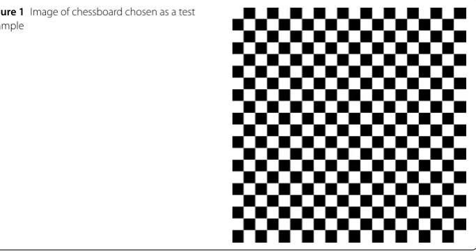
According to the comment above we consider as an example of image a chessboard (Fig.1) with 2048 pixels for both coordinates (M=N= 2048) having 20 alternating boxes for each row or column of the chessboard. The usual 8-bit gray scale representation is considered for the color, so thatB= 8. We generated reduced resolution images at com-pression ratiosρ= 4, 9, 16, 25, 36 (B= 2, . . . , 6).
The value of SNR for bi-linear, bi-cubic, bi-spline, Shepard (s= 4, 6),Gα,4M,N,Gα,6M,N op-erators, withα= 1.1, 1.3, 2, 3, 5, 10 and compression ratioρ= 4, 9, 16, 25, 36, is shown in Table1.
We can see that the Shepard–Gupta-type operator (18) gives the best results at any com-pression ratio and that accuracy improves whenαincreases.
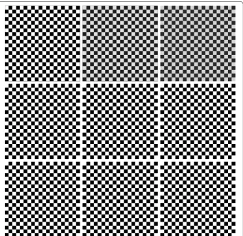
Figure2shows the decompressed images for bi-linear, bi-cubic, bi-spline, Shepard (s= 4, 6),Gα,4M,N,Gα,6M,N operators,α= 2, 10, obtained for compression ratio 25. We notice the gray color of the truly white boxes in the chessboard for bi-spline and bi-cubic operators (middle and right upper plots). It is due to overshoots (pixels having intensities greater than 1) and undershoots (pixels with intensity less than 0). As is well known these artifacts are particularly deleterious for images. Bi-linear and Shepard–Gupta-type operators being stable in the Fejér sense do not suffer from this artifact.
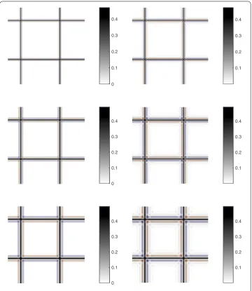
To better appreciate this artifact and differences among the above methodologies, Fig.3
shows the (absolute) error of the decompressed images for only bi-cubic and bi-spline op-erators at different compression ratios (ρ= 9, 25, 49), since the other operators are not af-fected by the overshoot-undershoot artifact. Overshoots and undershoots are represented with red and blue color, respectively.
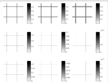
[image:9.595.134.476.554.734.2]A full assessment of all considered methods is graphically given in Fig.4 in a partic-ularization of Fig.3. The figure shows the smaller error (higher SNR) achieved by the Shepard–Gupta-type method.
Table 1 SNR of the decompressed images for the Chessboard test example at compression ratio ρ= 4, 9, 16, 25, 36 and for bi-linear, bi-cubic, bi-spline, Shepard (s= 4, 6),Gα,4M,N,Gα,6M,Noperators, α= 1.1, 1.3, 2, 3, 5, 10. The higher SNR, the more accurate the methodology
Method ρ= 4 ρ= 9 ρ= 16 ρ= 25 ρ= 36
Original Shepard (s= 4) 79.6 77.4 76.0 75.0 74.0
G1.1,4M,N 80.3 78.1 76.7 75.6 74.6
G1.3,4M,N 81.6 79.2 77.8 76.7 75.7
G2,4M,N 85.3 82.4 80.7 79.5 78.3
G3,4M,N 89.8 85.8 83.7 82.3 81.0
G5,4M,N 98.5 91.7 88.5 86.5 84.7
G10,4M,N 120.4 106.4 99.7 95.5 92.2
Original Shepard (s= 6) 82.0 79.6 78.1 77.0 76.0
G1.1,6M,N 82.9 80.3 78.8 77.7 76.6
G1.3,6M,N 84.4 81.6 80.0 78.8 77.7
G2,6M,N 89.1 85.3 83.3 82.0 80.6
G3,6M,N 95.6 89.8 87.0 85.2 83.6
G5,6M,N 108.8 98.5 93.7 90.7 88.3
Bi-linear 73.3 72.0 70.3 69.4 68.5
Bi-cubic 73.8 72.0 70.8 69.9 69.0
Bi-spline 73.2 71.4 70.2 69.3 68.4
[image:10.595.122.477.342.686.2]Figure 3Error of the decompressed images for the chessboard test example for the considered methods (particular). From top to bottom and left to right bi-cubic and bi-spline forρ= 9, bi-cubic and bi-spline for
ρ= 25, bi-cubic and bi-spline forρ= 49. Blue and red colors indicate undershoots and overshoots, respectively
3 Conclusions
Figure 4Error of the decompressed images for the Chessboard test example for the considered methods (particular). From top to bottom and left to right: bi-linear, bi-cubic, bi-spline, Shepard (s= 4),G2,4M,N,G10,4M,N, Shepard (s= 6),G2,6M,N,G10,6M,Noperators for compression ratioρ= 25. Blue and red colors indicate undershoots and overshoots, respectively
Acknowledgements
The authors are grateful to an anonymous referee for his/her stimulating remarks that improved the paper.
Funding
The authors declare that they have no specific funds to acknowledge.
Availability of data and materials
Data sharing not applicable to this article as no datasets were generated or analyzed during the current study.
Competing interests
The authors declare that they have no competing interests.
Authors’ contributions
BDV introduced the variant of the operator and studied the corresponding approximation results. UA applied such operator to the image compression problem. Both authors read and approved the final manuscript. All authors read and approved the final manuscript.
Author details
1Consiglio Nazionale delle Ricerche, Istituto per la Microelettronica e Microsistemi, Napoli, Italy.2Dipartimento di
Matematica, Università degli Studi La Sapienza, Roma, Italy.
Publisher’s Note
Springer Nature remains neutral with regard to jurisdictional claims in published maps and institutional affiliations.
Received: 6 April 2018 Accepted: 17 August 2018
References
1. Della Vecchia, B.: Direct and converse results by rational operators. Constr. Approx.12, 271–285 (1996).
https://doi.org/10.1007/BF02433043
2. Della Vecchia, B., Mastroianni, G.: Pointwise simultaneous approximation by rational operators. J. Approx. Theory65, 140–150 (1991).https://doi.org/10.1016/0021-9045(91)90099-V
4. Della Vecchia, B., Mastroianni, G., Vertesi, P.: Direct and converse theorems for Shepard rational approximation. Numer. Funct. Anal. Optim.17, 537–561 (1996).https://doi.org/10.1080/01630569608816709
5. Somorjai, G.: On a saturation problem. Acta Math. Acad. Sci. Hung.32, 377–381 (1978).
https://doi.org/10.1007/BF01902372
6. Szabados, J.: On a problem of R DeVore. Acta Math. Acad. Sci. Hung.27, 219–223 (1976).
https://doi.org/10.1007/BF01896777
7. Vertesi, P.: Saturation of the Shepard operator. Acta Math. Hung.72(4), 307–317 (1996).
https://doi.org/10.1007/BF00114543
8. Allasia, G.: A class of interpolatory positive linear operators: theoretical and computational aspects. In: Approximation Theory, Wavelets and Applications. NATO ASI Series C, vol. 454, pp. 1–36 (1995).
https://doi.org/10.1007/978-94-015-8577-4_1
9. Amato, U., Della Vecchia, B.: New results on rational approximation. Results Math.67, 345–364 (2015).
https://doi.org/10.1007/s00025-014-0420-4
10. Amato, U., Della Vecchia, B.: Modelling by Shepard-type curves and surfaces. J. Comput. Anal. Appl.20, 611–634 (2016)
11. Amato, U., Della Vecchia, B.: Weighting Shepard-type operators. Comput. Appl. Math.36, 885–902 (2016).
https://doi.org/10.1007/s40314-015-0263-y
12. Amato, U., Della Vecchia, B.: Inequalities on Shepard-type operators. J. Math. Inequal.12(2), 517–530 (2018) 13. Amato, U., Della Vecchia, B.: Rational operators based onq-integers. Results Math.72(3), 1109–1128 (2017).
https://doi.org/10.1007/s00025-017-0682-8
14. Wu, Y.-H., Hung, M.-C.: Comparison of spatial interpolation techniques using visualization and quantitative assessment. In: Hung, M. (ed.) Applications of Spatial Statistics, pp. 17–34. IntechOpen, London (2016).
https://doi.org/10.5772/65996
15. Li, L., Zhou, X., Kalo, M., Piltner, R.: Spatiotemporal interpolation methods for the application of estimating population exposure to fine particulate matter in the contiguous U.S. and a real-time web application. Int. J. Environ. Res. Public Health13, 749 (2016).https://doi.org/10.3390/ijerph13080749
16. Hammoudeh, M., Newman, R., Dennett, C., Mount, S.: Interpolation techniques for building a continuous map from discrete wireless sensor network data. Wirel. Commun. Mob. Comput.13, 809–827 (2013).
https://doi.org/10.1002/wcm.1139
17. Szalkai, I., Sebestyén, A., Della Vecchia, B., Kristóf, T., Kótai, L., Bódi, F.: Comparison of 2-variable interpolation methods for predicting the vapour pressure of aqueous glycerol solutions. Hung. J. Ind. Chem.43, 67–71 (2015).
https://doi.org/10.1515/hjic-2015-0011
18. Gupta, V.: The Bézier variant of Kantorovich operators. Comput. Math. Appl.47, 227–232 (2004).
https://doi.org/10.1016/S0898-1221(04)90019-3
19. Gupta, V.: Simultaneous approximation for Szasz–Mirakyan–Durrmeyer operators. J. Math. Anal. Appl.328, 101–105 (2007)
20. Gupta, V., Do ˆgru, O.: Approximation of bounded variation functions by a Bézier variant of the Bleimann, Butzer, and Hahn operators. Int. J. Math. Math. Sci.2006, Article ID 37253 (2006).https://doi.org/10.1155/IJMMS/2006/37253
21. Gupta, V., Karsli, H.: Rate of convergence for the Bézier variant of the MKZD operators. Georgian Math. J.14(4), 651–659 (2007)
22. Gupta, V., Lupas, A.: On the rate of approximation for the Bézier variant of Kantorovich–Balazs operators. Gen. Math.
12, 3–18 (2004)
23. Gupta, V., Vasishtha, V., Gupta, M.K.: Rate of convergence of the Szasz–Kantorovich–Bézier operators for bounded variation functions. Publ. Inst. Math.72(80), 137–143 (2002).https://doi.org/10.2298/PIM0272137G
24. Gupta, V., Zeng, X.: Rate of approximation for the Bézier variant of Balazs Kantorovich operators. Math. Slovaca57(4), 349–358 (2007).https://doi.org/10.2478/s12175-007-0029-0
25. Zeng, X.M., Gupta, V.: Rate of convergence of Baskakov-Bézier type operators for locally bounded functions. Comput. Math. Appl.44, 1445–1453 (2002).https://doi.org/10.1016/S0898-1221(02)00269-9
26. Gordon, W.J., Wixon, J.A.: Shepard’s method of “Metric Interpolation” to bivariate and multivariate interpolation. Math. Compet.32, 253–264 (1978).https://doi.org/10.2307/2006273
27. Szalkai, I., Della Vecchia, B.: Finding better weight functions for generalized Shepard’s operator on infinite intervals. Int. J. Comput. Math.88, 2838–2851 (2011).https://doi.org/10.1080/00207160.2011.559542
28. Totik, V.: Approximation by Bernstein polynomials. Am. J. Math.116(4), 995–1018 (1994).
https://doi.org/10.2307/2375007
29. Ditzian, Z., Totik, V.: Moduli of Smoothness. Springer, New York (1987).https://doi.org/10.1007/978-1-4612-4778-4
30. Hermann, T., Vertesi, P.: On the method of Somorjai. Acta Math. Hung.54(3–4), 253–262 (1989).