A Novel TOPSIS MABAC Method for Multi attribute Decision Making with Interval Neutrosophic Set

2019 International Conference on Computation and Information Sciences (ICCIS 2019) ISBN: 978-1-60595-644-2

A Novel TOPSIS-MABAC Method for

Multi-attribute Decision Making with

Interval Neutrosophic Set

Xiangxiang Cui and Dongsheng Xu

ABSTRACT

Interval neutrosophic Set is a useful tool to describe the indeterminate, inconsistent, and incomplete information. This paper presents the application of the new TOPSIS-MABAC model with interval neutrosophic number in multi-attribute decision-making problem. In this model, the combined weight of attributes is obtained based on TOPSIS method while the best alternatives by MABAC method. Firstly, some definitions of INS are given in this paper. Secondly, the objective attribute weights are determined by TOPSIS method, and then a combined attribute weight is proposed. Finally an extended MABAC method is developed to rank the alternatives in multi-attribute decision-making problem and an illustrative examples are given to demonstrate the practicality and effectiveness of this new method.

1. INTRODUCTION

Multi-attribute decision making (MADM) problem [1] is an important part of modern decision science. Because of the fuzziness of human thinking and the complexity and uncertainty of objective things, it is difficult for a decision maker to express the evaluation value of an attribute with a crisp value. For this reason, fuzzy value is a better choice to describe these fuzzy information.

Fuzzy set (FS) is characterized by membership function and was firstly proposed by Zadeh [2]. On this basis, Atanassov [3], [4] proposed the intuitionistic fuzzy set (IFS) with membership function and non-membership function, and used it to solve

Xiangxiang Cui, School of Science, Southwest Petroleum University, Chengdu 610500, China. Email: [email protected]

some decision problems. Then some aggregation operators based on these were proposed by Xu [5-6] and some methods for MADM with IFS were proposed in [7-8].Furthermore, Atanassov and Gargov [4,9] extended the membership function and non-membership function to interval numbers and proposed interval-value intuitionistic fuzzy set (IVIFS).But IFS and IVIFS can only deal with incomplete information, but not uncertain and inconsistent information.

Therefore, Smarandache [10], [11] firstly proposed Neutrosophic Set (NS), however NS was mainly put forward from a philosophical viewpoint. So Wang et al. [12] proposed Single-valued Neutrosophic Set (SVNS) with the corresponding properties and operation rules. Similar to IVIFS, Wang et al. [13] proposed Interval Neutrosophic Set (INS) and gave the set-theoretic operators of INS.

In this paper, we propose the TOPSIS-MABAC method, which is a combined method under interval neutrosophic environment for solving MADM problem. The specific arrangements of this article are structured as follows. In section 2, we briefly introduce some concepts and definitions of INS. In Section 3, we propose TOPSIS method to determine the objective attribute weights and the combined weights, and then use MABAC method to obtain the best alternative. In Section 4, we give an example to illustrate the application of proposed method. In Section 5, we make a conclusion.

2. PRELIMINARIES OF NEUTROSOPHIC

2.1 Neutrosophic Set

Definition 1: Let

X

be a space of points (objects), with a generic element in

X

denoted by

x

. A neutrosophic setAin

X

is characterized by a truth-membership function T xA

 

, an indeterminacy-membership function IA

 

x , and a

falsity-membership function F_A

 

x ，where T x_A

 

，I_A

 

x and F_A

 

x are real standard or nonstandard subsets of _0 ,1 _, that is T_A

 

x :X  0,1_ ，

 

: 0,1

A

I x X   _ and FA

 

x :X 0,1

 

 

  .

There is no restriction on the sum of

T x

_A

( )

,

I x

_A

( )

,and

F x

_A

( )

, so

 

 

 

0 supT xA supIA x supF xA 3

 _{   } 

.

2.2 Interval Neutrosophic Set

Definition 2: Let

X

be a space of points (objects), with a generic element in

X

truth-membership function T x_A

 

, an indeterminacy-membership function I_A

 

x

and a falsity-membership functionFA

 

x , then A can be denoted by

 

 

 



, A , A , A



A x T x I x F x xX ,

WhereT_A

 

x  T_AL

 

x T, _AU

 

x _,I_A

 

x  I_AL

 

x I, U_A

 

x _,

 

L

 

, U

 

A A A

F x  F x F x _ 

 

0,1 for every

x

in

X

,and

 

 

 

0 sup T_A x supI_A x supF x_A 3.

For convenience, we refer toA TA,IA,FA  TAL,TAU  , IAL,IAU  , FAL,FAU

as INN.

Definition 3: The complement of _A is denoted by c

A and is defined as

, , 1 ,1 , ,

c L U U L L U

A A A A A A

A  _F F _{ }  I I _{ } T T _

Definition 4: Let _A and _B be two INNs, then the normalized Euclidean distance between A and Bis

  1





 

2

 

2

 

2

 

2

 

2



2



,

6

L L U U L L U U L L U U

A B A B A B A B A B A B

d A B  T T  T T  I I  I I  F F  F F (1)

Definition 5: Let _A be an INN, a score function S of _A is:

 

4

6

L L L U U U

A A A A A A

T I F T I F

S A       

Definition 6: Let A be an INN, an accuracy function

H

of A is:

 



 



2

L U L U

A A A A

T T F F

H A    

Definition 7: Let A and B be two INNs, S A

 

and S B

 

be the score functions, H A

 

and H B

 

be the accuracy functions, then if S A

   

S B ,

then A B ; if S A

   

S B ,then (1) if H A

 

H B

 

,then A B ;

3. TOPSIS-MABAC METHOD FOR INTERVAL NEUTROSOPHIC MADM PROBLEM

Let A



A A₁, ₂, ,A_m



be a set of alternatives, C 



C C₁, ₂, ,C_n



be a series

of attributes, and w



w w1, 2, ,wn



be the subjective weight of the attribute,

w

j

is the weight of the j-th attribute where wj

 

0,1 and 1

1 n

j j

w







. The interval neutr-

osophic number L, U , L, U , L, U ij ij ij ij ij ij ij

a  T T _{ } I I _{ } F F _ is the evaluated value of

A

_i

under

C

_j, then the decision matrix A

 

aij _{m n} is obtained. To get the optimal

alter-

Native (s), we propose the TOPSIS-MABAC method with INN.

Step 1: Normalization of the initial decision matrix. That is, normalized the

matrix A

 

aij _{m n} into

 

_ij



_ijNL, _ijNU, , _ijNL, _ijNU, , _ijNL, _ijNU,



m n _{m n}

R r T T I I F F

       _

 _{      } , where

, ;

, cos .

ij j c ij

ij j

a C is the benefit type attribuite r

a C is the t type attribuite

 

  _

 .

Step 2:Calculating the combined weight.

According to the normalized decision matrix, we can define the positive ideal so-

lution (PIS) and negative ideal solution (NIS) as following:

1 2

1 2

( , , , )

( , , , )

n

n

PIS R R R R

NIS R R R R

   

   

  

 

 

 (2)

Where









max , max , , min , min , , min , min ,

min , min , , max , max , , max , max ,

NL NU NL NU NL NU

j ij ij ij ij ij ij

i i i i

i i

NL NU NL NU NL NU

j _i ij _i ij ij ij ij ij

i i i i

R T T I I F F

R T T I I F F





 _{      }

      



   

 

 _{ }

    



for j1, 2, ,n.

①Determination of objective weight vector



o 



 

₁, ₂, ,



_n



.

1

( ) ( , )

n

i ij j j

j

e  d r R 







.So

1 1

( ) ( , )

m n

ij j j

i j

e  d r R 

 





represents the sum of the

weight distance between all the alternatives and PIS. Therefore, we can establish the model as follows:

1 1

1

min ( ) ( , )

. . 1, 0, 1, 2, ,

m n

ij j j

i j n

j j

j

e d r R

s t j n

             _     _{  } 





.

By constructing the Lagrange function, we can get 1

1 1 ( , ) ( , ) m ij j i

j n m

ij j j i

d r R

d r R        





. (3)

Similarly we can get 1

1 1 ( , ) ( , ) m ij j i

j n m

ij j j i

d r R

d r R        





. (4)

So the objective weight is



o 



 

₁, ₂, ,



_n



, where 1





2

j j j

 _ _

.

②Determination of combined weight

  





₁, ₂, ,



_n



, where

 

_j



_j





1





wj, for j 1, 2, ,n,and 0  1.

Step 3: Calculation of weighted normalized decision matrix

 

L,

ij _{m n} ij

V  v _  T U , L, U , L, U ij ij ij ij ij

T  _{ }I I  _{ }F F _ ,i1, 2, , ,n j1, 2, ,m, where









1 1 NL j,1 1 NU j ,

ij j ij ij ij

v  r  __  T   T  _

   

IijNL j , IijNU j ,

  

FijNL j , FijNU



j

   

   

   

    (5)

Step 4: Determination of the border approximation area matrixG

 

gj _1n.

 

1

   

1 1





1





1

1 1 , 1 , 1 1 1 ,1 1 1 ,

m m m m m

L _m U _m L _m U _m

m

j ij ij ij ij ij

i i i i i

g v T T I I

    

   

   _  _{ }       _

   





1





1

1 1 ,1 1

m m

L _m U _m

ij ij

F F

 

 

     

Step 5: Determination of the distance matrix D

 

dij _{m n} , where









,

0

,

ij j ij j

ij ij j

ij j ij j

d v g if v g

d if v g

d v g if v g

 



_ 

 



Step 6: Calculation of

Q

_i, where

1

n

i ij

j

Q d







.

Step 7: Ranking the alternatives according to the value of

Q

_i.The value of

Q

_iis larger, the alternative is better.

4. NUMERICAL EXAMPLE

There is an investment company which wants to invest a number of money in a

best option. There are four possible alternatives to invest the money:

A

₁,

A

₂,

A

₃and

4

A

. The investment company should take a decision according to the following

three attribute:

C

₁,

C

₂and

C

₃, where

C

₁and

C

₂are benefit-type attributes and

C

₃ is a cost-type attribute .The objective weight vector of the attribute is given by



0.35, 0.25, 0.4



w . The four possible alternatives are to be evaluated under the above three attribute by the form of INNs, as shown in the following interval neutrosophic decision matrix 𝐴:



 

 

 

 

 

 

 

 





 

 

 

 

 





 

 





 

 

 

 

 

 



0.4, 0.5 , 0.2, 0.3 , 0.3, 0.4 0.4, 0.6 , 0.1, 0.3 , 0.2, 0.4 0.7, 0.9 , 0.2, 0.3 , 0.4, 0.5

0.6, 0.7 , 0.1, 0.2 , 0.2, 0.3 0.6, 0.7 , 0.1, 0.2 , 0.2, 0.3 0.3, 0.6 , 0.3, 0.5 , 0.8, 0.9

0.3, 0.6 , 0.2, 0.3 , 0.3, 0.4 0.5, 0.6 , 0.2, 0.3 , 0.3, 0.4 0.4, 0.5 , 0.2, 0.

A



 





 

 





 

 





 

 



4 , 0.7, 0.9

0.7, 0.8 , 0.0, 0.1 , 0.1, 0.2 0.6, 0.7 , 0.1, 0.2 , 0.1, 0.3 0.6, 0.7 , 0.3, 0.4 , 0.8, 0.9

 

 

 

 

 

 

 

Then we use the proposed method to obtain the best alternative. Step1: Normalized the decision matrix and get the normalized matrix:



 

 

 

 

 

 

 

 





 

 

 

 

 

 

 

 





 

 

 

 

 

 



0.4, 0.5 , 0.2, 0.3 , 0.3, 0.4 0.4, 0.6 , 0.1, 0.3 , 0.2, 0.4 0.4, 0.5 , 0.7, 0.8 , 0.7, 0.9

0.6, 0.7 , 0.1, 0.2 , 0.2, 0.3 0.6, 0.7 , 0.1, 0.2 , 0.2, 0.3 0.8, 0.9 , 0.5, 0.8 , 0.3, 0.6

0.3, 0.6 , 0.2, 0.3 , 0.3, 0.4 0.5, 0.6 , 0.2, 0.3 , 0.3, 0.4 0.7, 0.9 , 0.6, 0.

R



 





 

 





 

 

 

 

 



8 , 0.4, 0.5

0.7, 0.8 , 0.0, 0.1 , 0.1, 0.2 0.6, 0.7 , 0.1, 0.2 , 0.1, 0.3 0.8, 0.9 , 0.6, 0.7 , 0.6, 0.7

 

 

 

 

 

 

 



 

 



1 0.7, 0.8 , 0.0, 0.1 , 0.1, 0.2

R  ,R1



0.3, 0.5 , 0.2, 0.3 , 0.3, 0.4

 

 



_

,



 

 



2 0.6, 0.7 , 0.1, 0.2 , 0.1, 0.3

R  ,R2



0.4, 0.6 , 0.2, 0.3 , 0.3, 0.4

 

 



 _

,



 

 



3 0.8, 0.9 , 0.5, 0.7 , 0.3, 0.5

R  ,R3



0.4, 0.5 , 0.7, 0.8 , 0.7, 0.9

 

 



_

. According to Eq.(3) and Eq.(4),we can get

1

0.4







,



₂



0.2

,



₃



0.4

,

1

0.3







,



₂



0.2

,



₃



0.5

Then the objective weight is obtained and denoted as



o 



0.35,0.2,0.45



, In this section, we set 0.7, so the combined weight is







0.35, 0.215, 0.435



.

Step 3:Calculation of the weighted normalized decision matrix V 

 

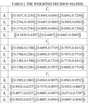
vij _{m n} which [image:7.612.147.451.321.673.2]

is shown in Table I.

TABLE I. THE WEIGHTED DECISION MATRIX.

1

C

1

A





0.1637, 0.2154 , 0.5693, 0.6561 , 0.6561, 0.7256

 

 





2

A





0.2744, 0.3439 , 0.4467, 0.5693 , 0.5693, 0.6561

 

 





3

A





0.1174, 0.2744 , 0.5693, 0.6561 , 0.6561, 0.7256

 

 





4

A





0.3439, 0.4307 , 0, 0.4467 , 0.4467, 0.5693

 

 





2

C

1

A





0.1040, 0.1788 , 0.6095, 0.7719 , 0.7075, 0.8212

 

 





2

A





0.1788, 0.2281 , 0.6095, 0.7075 , 0.7075, 0.7719

 

 





3

A





0.1385, 0.1788 , 0.7075, 0.7719 , 0.7719, 0.8212

 

 





4

A





0.1788, 0.2281 , 0.6095, 0.7075 , 0.6095, 0.7719

 

 





3

C

1

A





0.1993, 0.2603 , 0.8563, 0.9075 , 0.8563, 0.9552

 

 





2

A





0.5035, 0.6327 , 0.7379, 0.9075 , 0.5923, 0.8007

 

 





3

A





0.4077, 0.6327 , 0.8007, 0.9075 , 0.6713, 0.7397

 

 





Step 4: Calculating the border approximation area matrix G

 

gj _1n.According to

Eq.(6),we can get:



 

 



1 0.2064, 0.3059 , 0.4340, 0.5903 , 0.5903, 0.6750 g 



 

 



2 0.1465, 0.2020 , 0.6367, 0.7417 , 0.7045, 0.7980

g 



 

 



3 0.3788, 0.5067 , 0.8033, 0.8967 , 0.7511, 0.8648

g 

Step 5: Calculating the distance matrix D.

0.0812 0.0275 0.1387

0.0353 0.0311 0.1046

0.0800 0.0410 0.0809

0.2142 0.0472 0.0761

D

  

 

 

 



  

 

 

Step 6: Calculating

1

n

i ij

j

Q d







,i1, 2, , 4.We can get

1

0.2474

Q

 

,

Q

₂



0.1710

,

Q

₃

 

0.0431

,

Q

₄



0.3375

.

According the value of

Q

_i, we can get

A

₄

  

A

₂

A

₃

A

₁, so

A

₄ is the optimal alternative.

5. CONCLUSIONS

The aim of this paper is to introduce a new approach for MADM with interval n-eutrosophic set. At the beginning of this article, we briefly introduce some concepts and definitions of INS, and then propose TOPSIS method for determining the objective attribute weights and the combined weights. Next, in order to get the best alternative(s), we combined the MABAC method with the combined weights. Finally, we give an example to illustrate the application of proposed method. From the results we can see that this new method is useful for multi-attribute decision making problem.

REFERENCES

1. G. Buyukozkan, J. Arsenyan, and R. Da.2012. “Logistics tool selection with two-phase fuzzy multi criteria decision making: A case study for personal digital assistant selection,” Expert Systems with Applications, 39(1): 142-153.

4. Atanassov and K. T. 1989. “More on intuitionistic fuzzy sets,” Fuzzy Sets and Systems, 33(1): 37-45.

5. Z. Xu and R. R. Yager. 2006. “Some geometric aggregation operators based on intuitionistic fuzzy sets,” International Journal of General Systems, 35(4):417-433.

6. Z. Xu. 2007. “Intuitionistic fuzzy aggregation operators,” IEEE Transactions on Fuzzy Systems.,

15(6): 1179-1187.

7. X. Zhao and G. Wei. 2013. “Some intuitionistic fuzzy einstein hybrid aggregation operators and their application to multiple attribute decision making,” Knowledge-Based Systems. 37(2): 472-479.

8. G. Wei and X. Zhao. 2012. “Some induced correlated aggregating operators with intuitionistic fuzzy information and their application to multiple attribute group decision making,” Expert Systems with Applications, 39(2): 2026-2034.

9. K. T. Atanassov. 1994. “Operators over interval valued intuitionistic fuzzy sets,”Fuzzy Sets and Systems, 64(2): 159-174.

10. F. Smarandache. 1998. “Neutrosophy. Neutrosophic probability, set, and logic. Analytic synthesis and synthetic analysis,”Philosophy.

11. F. Smarandache. 1999. “A unifying field in logics: Neutrosophic logic,” Multiple-Value Logic, 8(3): 489-503.

12. H. Wang, F. Smarandache, Y. Zhang, and R. Sunderraman. 2010. “Single valued neutrosophic sets,” Review of the Air Force Academy, 10: 410-413.