2018 2nd International Conference on Modeling, Simulation and Optimization Technologies and Applications (MSOTA 2018) ISBN: 978-1-60595-594-0
Research on Uncertainty of Target Position
Estimation in Combat Simulation
Qi-hao HOU
*and Yi-ping YAO
College of System Engineering, National University of Defense Technology, 137 Yanwachi, Changsha, China
*Corresponding author
Keywords: Target Position Estimation, Area of Uncertainty, Extended Kalman Filter, Covariance Matrix, Dead Reckon.
Abstract. Target position estimation is valuable for sensor detection and weapon attack. However, there is position uncertainty due to sensor detection accuracy and environmental noise. In this paper, the uncertainty region is graphically represented by area of uncertainty (AOU), and the error ellipses represent the error dispersal of 2D target s position. Calculate AOU using Extended Kalman Filter
(EKF) algorithm and Dead Reckon (DR) algorithm. EKF covariance matrix is used for calculating AOU while estimating target position; The dead reckon algorithm realizes the update of AOU by calculating the time difference based on the last time’s AOU. Finally, it was implemented and operated in a naval combat system, which verifies the effectiveness of the algorithms.
Introduction
Battlefield target information is both the basis for command decision and the necessary for the combat unit to perform missions. In combat simulation, target information is acquired by various sensors. Based on this acquired information, the fusion system estimates and predicts the target's location, identification, threat classification, etc. Due to the uncertainty of measurement caused by sensor detection capability and environmental noise and the uncertainty of the target model used in the fusion center of simulation system, the obtained target state data is uncertain. This article focuses on the uncertainty of target location.
targets move and how AOUs grow between measurements. the two options are the Maneuvering Target Statistical Tracker (MTST) and Furthest-on Circles(FOC).
This paper mainly studies the uncertainty of target position estimation in com-bat simulation. Firstly, give the concept of AOU and its parameters, and introduces the role of AOU in moving target detection using multi-sensor; Secondly, briefly introduce the Extended Kalman Filter(EKF) and propose an AOU calculation method based on EKF covariance matrix;Thirdly, propose the Dead Reckon(DR) algorithm for AOU update; Finally, implement the two algorithms and verify the effectiveness of the algorithm by simulation experiments.
Area of Uncertainty (AOU)
Due to the low accuracy of multi-sensor measurement in combat simulation system, there is an error between the perceived track and the ground truth track. Command decisions are based upon generated, perceived tactical pictures, not the ground truth position of targets. Therefore, there is an uncertainty area of the target position.
The area of uncertainty (AOU) is defined as the minimum area having a specified probability of
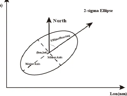
containing the measurement. The AOUs can be of three types: circular or ellipse, line of bearing, and bearing box. In combat simulation systems, the most common type of AOU is ellipse. the boundary of the calculated AOU represents an equal probability contour that contains the target with some specified probability. Under the assumption that the statistical distribution of positional errors follows a normal distribution, the AOUs include the target with probabilities of 39%, 86.5%, and 99%, which correspond to one, two, and three standard deviations respectively, in other words, represent 1-sigma, 2-sigma and 3-sigma ellipse respectively.
[image:2.595.198.420.447.615.2]As the Figure 1 shown, the measurement vector, the so-called ellipse contact report, comprises of the ellipse center coordinates (i.e. a target location), magnitudes of the semi-axes (Major_Axis and Minor_Axis), the ellipse orientation (Ellipse_Bearing), the associated time tag (AOU_Time) and the specified probability that the true location is within the ellipse region.
Figure 1. The AOU ellipse with 86.5% of probability confinement region.
AOU Generation Using Extended Klaman Filter(EKF)
Introduction to Kalman Filter(KF) and Extended Kalman Filter(EKF)
Kalman filtering is a method of estimating the current or future state of an evolving system from a sequence of “noisy” (i.e., inaccurate) measurements [11]. The Kalman filter recursively updates the mean of a system based on a series of measurements.
Stochastic Variables. The true state cannot be known exactly, so it is treated as a random variable. A Kalman filter represents the system state by a multivariate random normal variable X, with a mean
In this paper, only the 2-D target state is considered, and the target state variable contains two position information and two speed information.
Distance from reference location in latitude direction
Distance from reference location in longitude direction
Rate of change in distance from reference location in latitude direction
Rate of change i
X
n distance from reference location in longitude direction
Uncertainties are associated with both measurements and movement; Vand W are represented by the probability distributions V : N 0, R
and W : N 0,Q
.R the covariance of the measurement noise and Q is the covariance of the movement noise.Movement Matrix. The Kalman Filter algorithm uses the movement model to predict the next time state of the system X. The equation: X ΦX + Wrepresents movement model. The movement matrix
Φdescribes how the system’s state changes over time.
Measurement Matrix. The measurement model in Kalman Filter is used to correct the target state estimation based on the acquired measurement data. The measurement model is described as
Z = HX + V.The measurement matrix His used to estimate the target stateXbased on input Z. Kalman filter algorithm is mainly used to solve the linear filtering problem. Movement matrix Φ
and measurement matrix H are independent of state variables X. However, there are nonlinear filtering problems in multi-target multi-sensor tracking. For example, for bearing-only measurements, the measured angle is a nonlinear function of the state, requiring that an Extended Kalman Filter (EKF) be used.
AOU Calculation Based on EKF Covariance Matrix
This paper uses the EKF output covariance matrix to calculate the target AOU in the 2-D target state. The AOU calculated is a 2-Sigma ellipse which is an equal probability contour that contains the target state with probability equal to 2
1e or .865. Known by the second section, the ellipse has an inclination EllipseBearing, MajorAxis and MinorAxis. In calculating the dimensions of the ellipse we use the following matrix notation recalling that the output covariance matrix of the EKF is a 4 x 4 matrix consisting of 16 numbers of which we are only interested in using the upper 2 x 2 corner (four numbers). a h h b Σ 2 2
2 2 2
2 2
2 2 2
4
4 2 4
2
4
4 2 4
2
1 2
arctan 2
a b a b h
MajorAxis a b a b h
a b a b h
MinorAxis a b a b h
h EllipseBearing b a (1)
So, the size of AOU is calculated by:
AOU MajorAxis MinorAxis (2)
AOU Generation Using Dead Reckon(DR) Algorithm
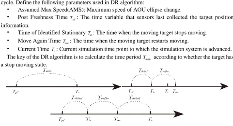
the change of AOU size. Assume that the moving target will stop moving in one sensor acquisition cycle. Define the following parameters used in DR algorithm:
• Assumed Max Speed(AMS): Maximum speed of AOU ellipse change.
• Post Freshness Time Tpf: The time variable that sensors last collected the target position
information.
• Time of Identified Stationary Tis: The time when the moving target stops moving.
• Move Again Time Tma: The time when the moving target restarts moving.
• Current Time Tc: Current simulation time point to which the simulation system is advanced. The key of the DR algorithm is to calculate the time period Tdelta according to whether the target has
[image:4.595.55.537.89.350.2]a stop moving state.
Figure 2. The three cases of calculating time period.
Case 1: Suppose the target does not stop moving, that is, from the last update time to the current time, the target does the uniform motion.
delta c pf
T T T (3) Case 2: Assume that the target has stopped moving, that is, the target will stop moving from the last update time to the current time.
delta is pf
T T T (4) If Tdelta 0, that is Tis Tpf, set Tdelta0, which means we got an updated hit on targets position after it
stopped moving.
Case 3: Assume that the target has stopped moving, that is, the movement is stopped at the time point Tis, and after a period of time Tbuffer, the target resumes the motion state.
1
2
1 2
delta is pf
ma pf buffer
delta c ma
delta delta delta
T T T
T T T
T T T
T T T
(5)
Assuming that the track estimation algorithm does not change the orientation of the AOU ellipse, the AOU attributes can be obtained according to Assumed Max Speed(AMS).
c pf delta
c pf delta
c pf
c c c
MajorAxis MajorAxis T ams
MinorAxis MinorAxis T ams
EllipseBearing EllipseBearing
AOU MajorAxis MinorAxis
(6)
Testing and Analysis
Assume that in a combined operation, the Red is tasked by a combination of naval ship formations and air force formations. The Blue consists of a cruiser and an air force flight formation. The simulation time is 10 hours and the time step to 10 minutes. Consider the Red N-1 cruiser to track and predict the flight track of the Blue F-1 combat aircraft. The fusion center is located on the N-1 cruiser and uses the radar signal (RADAR) and electromagnetic signal (ELINT) for target detection.
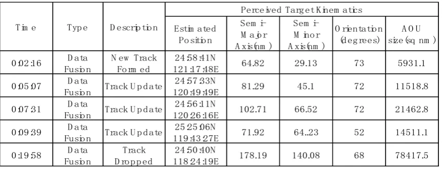
[image:5.595.154.445.197.296.2]The Blue consists of 24 F-1 combat aircraft. Each time two aircrafts are dis-patched to perform combat missions. When they are destroyed or reach the scheduled mission time, instead, the other two aircrafts will continue to complete the mission. The simulation process is shown as Figure 3. The simulation results are shown in Table 1 and Table 2.
[image:5.595.90.523.338.517.2]Figure. 3. Simulation process interface.
Table 1. The Perceived Information of F-1-000 By N-1 Cruiser Fusion Center
Estim ated Po sitio n
Sem i-M ajo r A xis(nm )
Sem i-M ino r A xis(nm )
O rientatio n (d eg rees)
A O U size(sq
nm )
0:01:03 D ata
Fusio n
N ew Track Fo rm ed
25:09:45N
121:25:56E 42.01 39.56 161 5220.81
0:02:16 D ata
Fusio n Track U p d ate
24:59:44N
120:57:13E 64.85 29.16 71 5941.6
0:05:07 D ata
Fusio n Track U p d ate
24:58:34N
120:29:18E 81.32 45.14 70 11533.6
0:08:48 D ata
Fusio n Track U p d ate
24:41:09N
120:06:30E 87.39 50.17 67 13775.6
0:09:48 D ata
Fusio n Track U p d ate
24:36:45N
119:58:03E 86.67 48.91 68 13316.1
0:20:06 D ata
Fusio n Track D ro p p ed
23:51:43N
118:30:45E 178.19 140.43 68 78613.1
Tim e Typ e D escrip tio n
Perceived Targ et Kinem atics
Table 2. The Perceived Information of F-1-001 By N-1 Cruiser Fusion Center
Estim ated Po sitio n
Sem i-M ajo r A xis(nm )
Sem i-M ino r A xis(nm )
O rientatio n (d eg rees)
A O U size(sq nm )
0:02:16 D ata
Fusio n
N ew Track Fo rm ed
24:58:41N
121:17:48E 64.82 29.13 73 5931.1
0:05:07 D ata
Fusio n Track U p d ate
24:57:33N
120:49:49E 81.29 45.1 72 11518.8
0:07:31 D ata
Fusio n Track U p d ate
24:56:11N
120:26:16E 102.71 66.52 72 21462.8
0:09:39 D ata
Fusio n Track U p d ate
25:25:06N
119:43:27E 71.92 64..23 52 14511.1
0:19:58 D ata
Fusio n
Track D ro p p ed
24:50:40N
118:24:19E 178.19 140.08 68 78417.5
Tim e Typ e D escrip tio n
Perceived Targ et Kinem atics
[image:5.595.84.515.542.707.2]the aircraft. Simulation experiments verify the feasibility and accuracy of the two algorithms in engineering implementation.
Summary
In this paper, Area of Uncertainty (AOU) is defined as the minimum area having a specified probability of containing the measurement. AOU has attributes such as Major_Axis, Minor_Axis, Ellipse_Bearing, AOU_Time and Assumed Max Speed (AMS). Due to the nonlinear properties of the target position uncertainty problem, this paper proposes an AOU calculation method based on EKF. Dead Reckon(DR) algorithm that is based on assumed maximum speed (AMS) is also proposed. Calculate the time difference according to whether the target stops motion, so as to update the current time AOU based on the AOU size at the post freshness time. Finally, two algorithms are implemented in a naval combat system, and the effectiveness of the algorithms are verified according to the expected running results.
References
[1] Lu Dai-Jun, Xia Xue-Zhi, Zhang Zi-He, Sha Ji-Chang. The Graphical Representation of Target Position Uncertainty [J]. Fire Control and Command Control, 2006, 31(9):58-60.
[2] Lu Dai-Jun, Xia Xue-Zhi, Zhang Zi-He. Target Damage Probability Calculation Method Based on Target Position and Weapon Landing Point Uncertainty Model [C]//Uncertain system annual meeting. 2005.
[3] Sun N. Estimation of area of uncertainty for moving target tracking[C]// International Conference on Mechatronic Sciences, Electric Engineering and Computer. IEEE, 2013:947-951.
[4] Mann J J. ASW Fusion on a PC[J]. Thesis Collection, 2004.
[5] Valerio S J. Probability of Kill for VLA ASROC Torpedo Launch[J]. Thesis Collection, 2009.
[6] Pabelico J C. Automating ASW Fusion[J]. Thesis Collection, 2011.
[7] Hadzagic M. Bayesian approaches to trajectory estimation in maritime surveillance[J]. 2010.
[8] Torrieri D J. Statistical Theory of Passive Location Systems[J]. Aerospace & Electronic Systems IEEE Transactions on, 1984, AES-20(2):183-198.
[9] Wang Kui, Zhao Zhong-wen. Evaluation of anti-terrorism’s efficiency on sea based on information cognition. Computer Engineering and Application, 2009-11, 45: 210-213.
[10] Ge Q, Liu L, Wang Y. An approach to estimate the closed-loop poles distribution area of uncertain system[C]// Control Conference. IEEE, 2015:198-204.
[11] Welch G, Bishop G. An Introduction to the Kalman Filter[J]. Course Notes 8 of ACM SIGGRAPH 2001, 1995, 8(7):127-132.