R E S E A R C H
Open Access
Bounding the
HL-index of a graph:
a majorization approach
Gian Paolo Clemente
*and Alessandra Cornaro
*Correspondence:
gianpaolo.clemente@unicatt.it Department of Mathematics and Econometrics, Catholic University, Milan, Italy
Abstract
In mathematical chemistry, the median eigenvalues of the adjacency matrix of a molecular graph are strictly related to orbital energies and molecular orbitals. In this regard, the difference between the occupied orbital of highest energy (HOMO) and the unoccupied orbital of lowest energy (LUMO) has been investigated (see Fowler and Pisansky in Acta Chim. Slov. 57:513-517, 2010). Motivated by the HOMO-LUMO separation problem, Jakliˇcet al.in (Ars Math. Contemp. 5:99-115, 2012) proposed the notion ofHL-index that measures how large in absolute value are the median eigenvalues of the adjacency matrix. Several bounds for this index have been provided in the literature. The aim of the paper is to derive alternative inequalities to bound theHL-index. By applying majorization techniques and making use of some known relations, we derive new and sharper upper bounds for this index. Analytical and numerical results show the performance of these bounds on different classes of graphs.
Keywords: graph eigenvalue; median eigenvalue; majorization; HOMO-LUMO
1 Introduction
The Hückel molecular orbital method (HMO) (see []) is a methodology for the determi-nation of energies of molecular orbitals ofπ-electrons. It has been shown thatπ-electron energy levels are strictly related to graph eigenvalues. For this reason, graph spectral the-ory became a standard mathematical tool of HMO thethe-ory (see [–] and []). Among the variousπ-electron properties that can be directly expressed by means of graph eigenval-ues, one of the most significant is the so-called HOMO-LUMO separation, based on the gap between the highest occupied molecular orbital (HOMO) and the lowest unoccupied molecular orbital (LUMO). For more details as regards the HOMO-LUMO separation issue we refer the reader to [–] and [].
In some recent works, Fowler and Pisanski ([] and []) introduced an index of a graph that is related to the HOMO-LUMO separation. By analogy with the spectral radius, these authors proposed the notion of the HOMO-LUMO radius which measures how large in absolute value may be the median eigenvalues of the adjacency matrix of a graph. At the same time, an analogous definition is given in [] that introduces theHL-index of a graph. Several bounds for this index have been proposed for some classes of graphs in [] and []. Recently in [] the authors provided some inequalities on theHL-index through the energy index.
The contribution of this paper is along those lines: we derive, through a methodology based on majorization techniques (see [–] and []), new bounds on the median eigen-values of the normalized Laplacian matrix. Consequently, given the relation between the normalized Laplacian matrix and the adjacency matrix eigenvalues, we provide some new bounds for theHL-index. In particular, we employ a theoretical methodology proposed by Bianchi and Torriero in [] based on nonlinear global optimization problems solved through majorization techniques. These bounds can also be quantified by using the nu-merical approaches developed in [] and [] and extended for the normalized Laplacian matrix in [] and in [].
Furthermore, another approach to derive new bounds makes use of the relation between
HL-index and energy index. In particular, we take advantage of an existing bound on the energy index (see []) depending on additional information on the first eigenvalue of the adjacency matrix. This additional information is obtained here by using majorization techniques in order to provide new inequalities for theHL-index of bipartite and non-bipartite graphs.
The paper is organized as follows. In Section some notations and preliminaries are given. Section concerns the identification of new bounds for theHL-index. In partic-ular, in Section ., by the fact that the eigenvalues of normalized Laplacian matrix and adjacency matrix are related, we localize the eigenvalues of the normalized Laplacian ma-trix via majorization techniques. In Section . we find a tighter alternative upper bound for theHL-index by using the relation with energy index provided in [] and an existing bound on energy index proposed in []. Section shows how the bound determined in Section . improves those presented in the literature.
2 Notations and preliminaries
In this section we first recall some basic notions on graph theory (for more details re-fer to []) and on theHL-index. Considering a simple, connected and undirected graph
G= (V,E) whereV={, , . . . ,n}is the set of vertices andE⊆V×V the set of edges,
|E|=m. The degree sequence ofGis denoted byπ= (d,d, . . . ,dn) and it is arranged in
non-increasing orderd≥d≥ · · · ≥dn, wherediis the degree of vertexi.
LetA(G) be the adjacency matrix ofGandD(G) be the diagonal matrix of vertex de-grees. The matrix L(G) =D(G) –A(G) is called Laplacian matrix of G, while L(G) =
D(G)–/L(G)D(G)–/ is known as the normalized Laplacian. Let λ
≥λ ≥ · · · ≥λn,
μ≥μ≥ · · · ≥μnandγ≥γ≥ · · · ≥γnbe the set of real eigenvalues ofA(G),L(G),
andL(G), respectively. The following properties of spectra ofA(G) andL(G) hold:
n
i=
λi=tr
A(G)= ;
n
i=
λi =trA(G)= m; λ≥ m
n ;
n
i=
γi=tr
L(G)=n;
n
i=
γi=trL(G)=n+ (i,j)∈E
didj
; γn= ;γ≤.
The eigenvalues involved in the HOMO-LUMO separation are λH and λL, where
H=n+ andL=n+ .
TheHL-index of a graph is defined in [] as
R(G) =max|λH|,|λL|
In the following, we list some well-known results on this index. In [] the authors show that, for every connected graph,R(G) is bounded as
≤R(G)≤d. ()
Other bounds have been found for special classes of graphs in [, ] and []. Finally, [] shows that for a simple connected graph
≤R(G)≤E(G)
n , ()
whereE(G) =ni=|λi|is the energy index of graph introduced by Gutman in [].
By (), the following bounds depending onnandmhave been derived in [] for non-bipartite and non-bipartite graphs, respectively:
≤R(G)≤m
n +
n
(n– )
m–m
n
, ()
≤R(G)≤m
n +
n
(n– )
m–m
n
. ()
Other bounds have been proposed in [] for non-bipartite and bipartite graphs depend-ing only onn:
≤R(G)≤
√ n+
()
and
≤R(G)≤
√ n+√
√
. ()
We now recall the following results regarding nonlinear global optimization problems solved through majorization techniques. We refer the reader to [] for more details as regards majorization techniques and for the proofs of Lemma and Theorems and recalled in the following.
Letgbe a continuous function, homogeneous of degreep, real, and strictly Schur-convex (see [] for the definition of Schur-convex functions and related properties). Let us as-sume
S=∩ x∈RN+ :g(x) =
N
i=
xpi =b
,
wherepis an integer greater than ,b∈R, and
= x∈RN+ :x≥x≥ · · · ≥xN, N
i=
xi=a
.
Lemma Fix b∈Rand consider the set S.Then either b=Napp– or there exists a unique integer≤h∗<N such that
ap
(h∗+ )p– <b≤
ap
(h∗)p–,
where h∗=p–ap
b.
We can now deduce upper and lower bounds forxh (withh= , . . . ,N) by solving the
following optimization problemsP(h) andP∗(h):
max(xh) subject to x∈S, (P(h))
min(xh) subject to x∈S. (P∗(h))
Theorem The solution of the optimization problem P(h)is(Na)if b=Napp–.If b= a p
Np–, the solution of the optimization problem P(h)isα∗where
. forh>h∗,α∗is the unique root of the equation
f(α,p) = (h– )αp+ (a–hα+α)p–b= ()
inI= (,ah];
. forh≤h∗,α∗is the unique root of the equation
f(α,p) =hαp+ (a–hα)
p
(N–h)p––b= ()
inI= (a N,
a h].
Theorem The solution of the optimization problem P∗(h)is(Na)if b=Napp–.If b= a p
Np–, the solution of the optimization problem P∗(h)isα∗where
. forh= ,α∗is the unique root of the equation
f(α,p) =h∗αp+a–h∗αp–b= ()
inI= (h∗a+,ha∗];
. for <h≤(h∗+ ),α∗is the unique root of the equation
f(α,p) = (N–h+ )αp+(a– (N–h+ )α)
p
(h– )p– –b= ()
inI= (,Na];
. forh> (h∗+ ),α∗is zero.
3 Some new bounds for theHL-index via majorization techniques
3.1 Bounds on median eigenvalues of the normalized Laplacian matrix
information on median eigenvalues and the interlacing between eigenvalues of normalized Laplacian and adjacency matrices turned out to be a handy tool for bounding theHL-index for both non-bipartite and bipartite graphs. According to [] (see Theorem ..), the fol-lowing relations hold:
|λn–k+|
d ≤ |
–γk| ≤|
λn–k+|
dn
. ()
Proposition For a simple,connected,and non-bipartite graphs
≤R(G)≤dmax
| –α|,| –β|,| –α|,| –β|
()
when n is even with
α=
n–
n+
n–
n
b(n– ) –n
,
β=
n–
n–
n–
n
b(n– ) –n
,
α=
n–
n+
(n– ) (n+ )
b(n– ) –n
,
β=
n n–
–
b(n– ) –n
n(n– )
,
and
≤R(G)≤dmax
| –α|,| –β|
()
when n is odd with
α=
n–
n+
(n– ) (n+ )
b(n– ) –n
, β=
n–
n–b(n– ) –n
.
Proof From (), we can easily derive the following bounds:
≤R(G)≤ dmax(| –γn+ |,| –γ n
|) ifnis even, d(| –γn+
|) ifnis odd.
()
By applying majorization, we are able to bound the median eigenvaluesγi (with i= n
,
n+ ,
n+
) considered in (). To this aim, we face the set:
Sb= γ ∈Rn–:
n–
i=
γi=n,g(γ) = n–
i=
γi=b=n+
(i,j)∈E
didj
.
It is well known that, for every connected graph of ordern(see []), we have
n– ≤
n
(i,j)∈E
didj
and, consequently,
n
n– ≤b< n, ()
where the left inequality is attained for the complete graphG=Kn.
It is noteworthy to see thatS
bis derived from the general setSwitha=n,N=n– ,
b=b, andap= . By Lemma we have for a non-complete graph
h∗=
n b
with
n
<h∗<n– . ()
We distinguish the following cases: . Consideringγn
forneven, by () we haveh<h
∗. Hence, by solving equation () of
Theorem , we can derive the unit rootαsuch asγn
≤α. Therefore
α=
n–
n+
n–
n
b(n– ) –n
.
In virtue of (), we havenn–≤α< with the left inequality attained only for the
complete graphG=Kn.
In a similar way, we can evaluate the valueβ≤γn
, through the solution of
equation () of Theorem (whereh<h∗+ ), where
β=
n–
n–
n–
n
b(n– ) –n
.
From (), we have
n–<β≤
n
n–with the right inequality attained only for the
complete graphG=Kn.
Havingβ≤γn ≤α, then| –γn| ≤max(| –α|,| –β|).
. Picking nowγn+
, whereh≤h
∗by equation () of Theorem we deduce
α=
n–
n+
(n– ) (n+ )
b(n– ) –n
.
Taking into account the lower bound ofβ≤γn+
, by () and forneven, we have h<h∗+ and then
β=
n n–
–
b(n– ) –n
n(n– )
.
In this case, we derive| –γn+
. For a graph withnodd number of vertices, we need to study onlyγn+ with β≤γn+
≤α, and we have by Theorem and Theorem , respectively:
α=
n–
n+
(n– ) (n+ )
b(n– ) –n
and
β=
n–
n–b(n– ) –n
,
whereh<h∗+ . Hence,| –γn+
| ≤max(| –α|,| –β|).
By using the bounds on the eigenvalues of the normalized Laplacian matrix computed
above, bounds () and () follow.
Proposition For a simple,connected and bipartite graphs with n even we have
≤R(G)≤d –βbip, ()
where
βbip= –
b
n– – .
Proof WhenGis bipartite, theHL-index is defined as
R(G) = |λn|=|λn+ | ifnis even,
ifnis odd. ()
In virtue of (), we can derive the following bound whennis even:
R(G)≤d| –γn|. ()
By applying majorization techniques, we are able to boundγn
considered in ().
To this aim, we now face the set
Sb= γ∈Rn–:
n–
i=
γi=n– ,g(γ) = n–
i=
γi=b=n+
(i,j)∈E
didj
–
.
By () andb=b– , we have
(n– )
n– ≤b< (n– ), ()
where the left inequality is attained for the complete graphG=Kn.
The setS
bis derived from the general setSwitha=n– ,N=n– ,b=b, andp= .
By Lemma we have for a non-complete graph
h∗=
(n– )
b
with
n
– <h
∗≤n– , ()
forneven.
We now considerγn :
. By (), we haveh≤h∗. In virtue of equation () of Theorem , we deduce the following upper bound:
αbip = +
n–
n
b
n– –
.
. In a similar way, we can evaluate the valueβbip≤γn
, whereh<h
∗+ . Applying
Theorem entails
βbip= –
b
n– – .
It is easy to show that| –αbip| ≤ | –βbip|. Hence bound () follows.
3.2 Bounds onR(G) through the energy index
In the following we obtain bounds on theHL-index starting from (). Our aim is to bound the energy index making use of additional information on the first eigenvalue ofA(G). In [] the authors show that, if a tighter boundkonλsuch asλ≥k≥nm is available, then the energy index for a non-bipartite graph is bounded as
E(G)≤k+
(n– )m–k,
while for a bipartite graph it is
E(G)≤k+
(n– )m– k.
In order to find the value ofk, we can introduce new variablesxi=λi, facing the set:
Sb= x∈Rn+:
n
i=
xi= m
.
In virtue of (), we are now able to derive the following bounds for non-bipartite and bipartite graphs, respectively.
Proposition
. For a simple,connected and non-bipartite graphG
R(G)≤ k
n+
n
. For a simple,connected and bipartite graphG
R(G)≤k
n +
n
(n– )m– k, ()
where,by means of Theorem,
k= +h∗
n+
m( +h∗) –n
h∗
, h∗=
n m
.
Remark Bounds () and () are tighter than or equal to () and (), respectively.
Proof of Proposition . Non-bipartite graphs
We start by proving that the condition(m–k)≥required in bound () is
always satisfied for simple and connected graphs.
We havek∈(nm,(n+√m–n)). Indeed, by the basic concepts of calculus it is
easy to see thatkincreases whenmincreases and thenh∗tends to . Hence,kis limited from above by
(n+
√
m–n)and where (n+
√
m–n)≤√mthe
required condition is satisfied.
We now show how bound () improves bound () presented in []. We need to prove that the following inequality holds:
k–m
n
≤
(n– )
m–m
n
–
(n– )m–k.
By simple algebraic rules we obtain
kn– km
n – mn+ m+ m
n
≤–
mn– m+k–knmn– m– m
n + m
n
. ()
The left-hand side term of () can be represented by
f(k) =kn– km
n – mn+ m+ m
n .
The functionf(k)is a convex parabola that assumes negative values in the range of
kwe are interested in. Indeed we havef(nm)≤andf(√m)≤.
Both sides of () being negative we can apply some basic concepts of algebra, getting
kn+k(mn– m) + m– mn+ m≥. ()
The functiont(k) =kn+k(mn– m) + m– mn+ mis again a convex parabola with vertex(m(–n n),
m(m–n)(n–)
n ). Both coordinates are less than zero
(then m(–nn)<nm). Havingt(nm) = m(n– m)( –n)≥, inequality () is
Therefore, bound () performs better than or equal to bound ().
Furthermore, we see that both bounds perform equally whenh∗=nm (i.e. nm is an integer). It is noteworthy that:
(a) whennis odd, nm is never an integer (nm =nm); (b) whennis even, n
m is an integer whenm= n
xwithx| n
,≤x≤
n
(wherex|
n
is shorthand for ‘xdivides n’). In this casek=nm and we derive bound (). . Bipartite graphs
As for non-bipartite graphs, we start by proving that the condition(m–k)≥
required in bound () is always satisfied for simple and connected graphs. In this caseh∗tends to for complete graphs (wherem≤n).
By some basic algebraic concepts, we see that(m–k)≥entails:
mh+ h– h– h+ +mnh– n– nh+n≥.
The functionf(m) =m(h+ h– h– h+ ) +m(nh– n– nh) +nis concave, decreasing, and non-negative on the intervalm∈(n,n). Therefore, the required condition is satisfied.
We now show how bound () improves bound () presented in []. We need to prove that the following inequality holds:
k–m
n
≤
(n– )
m–m
n
–
(n– )m– k.
By simple algebra, we have
mn– km+ m– mn+kn
≤–n
mn– m+ k– knmn– m– m
n + m
n
. ()
The left-hand side term of () can be represented by
f(k) =kn– km+ mn+ m– mn.
The functionf(k)is a convex parabola that assumes negative values in the range of
kwe are interested in. Indeed we havef(nm)≤andf(√m)≤. Both sides of () being negative, by some manipulations we obtain
kn+ km(n– ) + m+ m– mn≥. ()
The functiont(k) =kn+ km(n– ) + m+ m– mnis again a convex
parabola with vertex(m(–n n),m(m–n )(n–)
n ). Both coordinates are less than zero
(then m(–nn)<nm). Havingt(nm) =nm(n+ m(n– ))≥, inequality () is
satisfied.
Hence bound () performs better than or equal to bound ().
4 Numerical results
4.1 Non-bipartite graphs
In this subsection we compare our bounds ((), (), and ()) with those existing in the literature. We initially compute them for graphs generated by using the Erdös-Rényi (ER) model GER(n,q) (see [–] and []) where edges are included with probability
qindependent from every other edge. Graphs have been derived randomly by using the well-known package of R (see []) and by ensuring that the graph is connected. Table compares alternative upper bounds of R(G) evaluated for simulatedGER(n, .) graphs with different number of vertices. It is noteworthy that bound () has the best perfor-mance forn= , while bound () is the sharpest one in all other cases. However, the improvements are very slight with respect to bound () when large graphs are consid-ered.
We now extend the analysis to the same class of graphs but with varying the probabilityq. Two alternative values (q= . andq= ., respectively) have been tested in Tables and . In both cases bound () appears always as the tightest one. In particular, we observe significant differences with respect to other bounds when the number of edges increases. It is noticeable in Table how the improvement is very remarkable even for very large graphs.
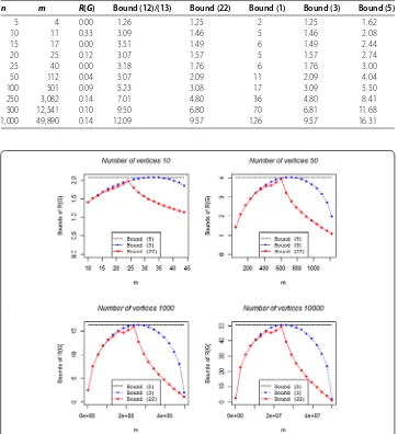
[image:11.595.119.478.456.574.2]We now focus on bounds (), (), and () that share the advantage of being dependent only onnand/orm. In Section ., it has been already proved that bound () is better than or equal to bound (). This result is obviously confirmed by Figure , where it is in-teresting to highlight how bound () strongly improves the other bounds for large values ofm.
Table 1 Upper bounds ofR(G) for graphs generated byGER(n, 0.5) model
n m R(G) Bound (12)/(13) Bound (22) Bound (1) Bound (3) Bound (5)
5 7 0.46 1.29 1.33 4 1.55 1.62
10 26 0.68 1.99 1.80 8 2.02 2.08
15 52 0.33 3.12 2.28 10 2.33 2.44
20 106 0.69 3.98 2.27 16 2.71 2.74
25 153 0.32 3.66 2.92 16 2.94 3.00
50 600 0.42 5.10 3.92 31 3.98 4.04
100 2,463 0.56 7.30 5.43 66 5.47 5.50
250 15,358 0.49 9.67 8.32 142 8.38 8.41
500 62,304 0.47 13.52 11.65 289 11.67 11.68
1,000 249,556 0.50 17.92 16.29 549 16.30 16.31
Table 2 Upper bounds ofR(G) for graphs generated byGER(n, 0.9) model
n m R(G) Bound (12)/(13) Bound (22) Bound (1) Bound (3) Bound (5)
5 9 1.00 1.41 1.17 4 1.62 1.62
10 43 1.00 1.61 1.15 9 1.90 2.08
15 102 1.00 1.57 1.13 14 2.00 2.44
20 176 1.00 2.19 1.22 19 2.30 2.74
25 284 1.00 2.09 1.19 24 2.32 3.00
50 1,154 1.00 2.72 1.24 49 2.79 4.04
100 4,669 0.94 3.39 1.31 98 3.41 5.50
250 29,507 0.96 4.63 1.42 246 4.57 8.41
500 118,482 0.95 6.00 1.57 488 5.91 11.68
[image:11.595.119.478.614.731.2]Table 3 Upper bounds ofR(G) for graphs generated byGER(n, 0.1) model
n m R(G) Bound (12)/(13) Bound (22) Bound (1) Bound (3) Bound (5)
5 4 0.00 1.26 1.25 2 1.25 1.62
10 11 0.33 3.09 1.46 5 1.46 2.08
15 17 0.00 3.51 1.49 6 1.49 2.44
20 25 0.12 3.07 1.57 5 1.57 2.74
25 40 0.00 3.18 1.76 6 1.76 3.00
50 112 0.04 5.07 2.09 11 2.09 4.04
100 501 0.09 5.23 3.08 17 3.09 5.50
250 3,082 0.14 7.01 4.80 36 4.80 8.41
500 12,541 0.10 9.50 6.80 70 6.81 11.68
1,000 49,890 0.14 12.09 9.57 126 9.57 16.31
Figure 1 Upper bounds ofR(G) for non-bipartite graphs with different number of vertices and edges.
4.2 Bipartite graphs
We now report in Table a comparison of alternative bounds derived for bipartite graphs, varying the number of vertices and edges. In some selected cases (i.e. n= ,m= and
n= ,m= ), our bound () performs better. In all the other cases, the tightest one is bound () as obtained in Section ..
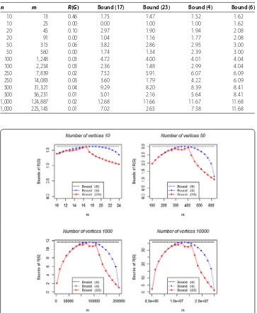
As for non-bipartite graphs, we can focus on bounds (), (), and () that can be com-puted without generating any graph. We observe in Figure how the bound () provides a significant improvement for higher values ofm. This result is also confirmed for very large graphs.
5 Conclusions
Table 4 Upper bounds ofR(G) for bipartite graphs
n m R(G) Bound (17) Bound (23) Bound (4) Bound (6)
10 13 0.46 1.75 1.47 1.52 1.62
10 25 0.00 0.00 1.00 1.00 1.62
20 45 0.10 2.97 1.90 1.94 2.08
20 91 0.00 1.04 1.16 1.77 2.08
50 315 0.06 3.82 2.86 2.95 3.00
50 560 0.00 1.74 1.34 2.39 3.00
100 1,248 0.03 4.72 4.00 4.01 4.04
100 2,254 0.03 2.36 1.48 2.99 4.04
250 7,839 0.02 7.52 5.91 6.07 6.09
250 14,083 0.03 3.60 1.79 4.22 6.09
500 31,321 0.04 9.29 8.20 8.39 8.41
500 56,231 0.01 5.01 2.16 5.64 8.41
1,000 124,887 0.02 12.68 11.66 11.67 11.68
[image:13.595.118.479.98.256.2]1,000 225,145 0.01 7.02 2.65 7.58 11.68
Figure 2 Upper bounds ofR(G) for bipartite graphs with different number of vertices and edges.
the interlacing between the eigenvalues of normalized Laplacian and adjacency matri-ces. On the other hand, new bounds are derived by making use of the relation between the HL-index and the energy index. Analytical and numerical results show the perfor-mance of these bounds on different classes of graphs. In particular, the bound related to the energy index performs better with respect to the best-known results in the liter-ature.
Competing interests
The authors declare that they have no competing interests.
Authors’ contributions
Acknowledgements
The authors are grateful to Anna Torriero and Monica Bianchi for useful advice and suggestions.
Endnote
a For values ofp> 2,b(and thenb
1andb2used in the sequel) depends on the graph’s structure and topology. So the procedure can be only numerically applied: we need to compute the eigenvalues of either adjacency or normalized Laplacian matrix, but this information allows one to directly obtainR(G). In this case, the evaluation of the bounds is useless.
Received: 13 July 2016 Accepted: 8 November 2016
References
1. Fowler, PW, Pisansky, T: HOMO-LUMO maps for chemical graphs. Acta Chim. Slov.57, 513-517 (2010) 2. Jakliˇc, G, Fowler, WP, Pisanski, T: HL-index of a graph. Ars Math. Contemp.5, 99-115 (2012)
3. Coulson, CA, O’Leary, B, Mallion, RB: Hückel Theory for Organic Chemists. Academic Press, London (1978) 4. Dias, JR: Molecular Orbital Calculations Using Chemical Graph Theory. Springer, Berlin (1993)
5. Graovac, A, Gutman, I, Trinajsti´c, N: Topological Approach to the Chemistry of Conjugated Molecules. Springer, Berlin (1977)
6. Gutman, I, Polansky, OE: Mathematical Concepts in Organic Chemistry. Springer, Berlin (1986)
7. Gutman, I, Trinajsti´c, N: Graph theory and molecular orbits. Totalπ-electron energy of alternant hydrocarbons. Chem. Phys. Lett.17, 535-538 (1972)
8. Graovac, A, Gutman, I: Estimation of the HOMO-LUMO separation. Croat. Chem. Acta53, 45-50 (1980) 9. Gutman, I: Note on a topological property of the HOMO-LUMO separation. Z. Naturforsch.35a, 458-460 (1980) 10. Gutman, I, Knop, JV, Trinajsti´c, N: A graph-theoretical analysis of the HOMO-LUMO separation in conjugated
hydrocarbons. Z. Naturforsch.29b, 80-82 (1974)
11. Kiang, YS, Chen, ET: Evaluation of HOMO-LUMO separation and homologous linearity of conjugated molecules. Pure Appl. Chem.55, 283-288 (1983)
12. Fowler, PW, Pisansky, T: HOMO-LUMO maps for fullerenes. MATCH Commun. Math. Comput. Chem.64, 373-390 (2010)
13. Mohar, B: Median eigenvalues of bipartite planar graphs. MATCH Commun. Math. Comput. Chem.70, 79-84 (2013) 14. Li, X, Li, Y, Shi, Y, Gutman, I: Note on the HOMO-LUMO index of graphs. MATCH Commun. Math. Comput. Chem.70,
85-96 (2013)
15. Bianchi, M, Cornaro, A, Palacios, JL, Torriero, A: Bounding the sum of powers of normalized Laplacian eigenvalues of graphs through majorization methods. MATCH Commun. Math. Comput. Chem.70(2), 707-716 (2013)
16. Bianchi, M, Cornaro, A, Palacios, JL, Torriero, A: New upper and lower bounds for the additive degree-Kirchhoff index. Croat. Chem. Acta86(4), 363-370 (2013)
17. Bianchi, M, Cornaro, A, Palacios, JL, Torriero, A: New bounds of degree-based topological indices for some classes of
c-cyclic graphs. Discrete Appl. Math.184, 62-75 (2015)
18. Bianchi, M, Cornaro, A, Torriero, A: Majorization under constraints and bounds of the second Zagreb index. Math. Inequal. Appl.16(2), 329-347 (2013)
19. Bianchi, M, Torriero, A: Some localization theorems using a majorization technique. J. Inequal. Appl.5, 443-446 (2000) 20. Clemente, GP, Cornaro, A: Computing lower bounds for the Kirchhoff index via majorization techniques. MATCH
Commun. Math. Comput. Chem.73, 175-193 (2015)
21. Cornaro, A, Clemente, GP: A new lower bound for the Kirchhoff index using a numerical procedure based on majorization techniques. Electron. Notes Discrete Math.41, 383-390 (2013)
22. Clemente, GP, Cornaro, A: New bounds for the sum of powers of normalized Laplacian eigenvalues of graphs. Ars Math. Contemp.11(2), 403-413 (2016)
23. Clemente, GP, Cornaro, A: Novel bounds for the normalized Laplacian Estrada index and normalized Laplacian energy. MATCH Commun. Math. Comput. Chem.77(3), 673-690 (2017)
24. Bianchi, M, Cornaro, A, Torriero, A: A majorization method for localizing graph topological indices. Discrete Appl. Math.161, 2731-2739 (2013)
25. Wilson, RJ: Introduction to Graph Theory. Addison Wesley, Harlow (1996)
26. Mohar, B: Median eigenvalues and the HOMO-LUMO index of graphs. J. Comb. Theory, Ser. B112, 78-92 (2015) 27. Gutman, I: The energy of a graph: old and new results. In: Betten, A, Kohnert, A, Laue, R, Wasserman, A (eds.) Algebraic
Combinatorics and Applications, pp. 196-211 (2011)
28. Marshall, AW, Olkin, I, Arnold, B: Inequalities: Theory of Majorization and Its Applications. Springer, Berlin (2011) 29. Cavers, M, Fallat, S, Kirkland, S: On the normalized Laplacian energy and general Randi´c indexR–1of graphs. Linear
Algebra Appl.433, 172-190 (2010)
30. Bianchi, M, Cornaro, A, Palacios, JL, Torriero, A: Bounds for the Kirchhoff index via majorization techniques. J. Math. Chem.51(2), 569-587 (2013)
31. Bollobás, B: Random Graphs. Cambridge University Press, London (2001)
32. Chung, FRK, Lu, L, Vu, V: The spectra of random graphs with given expected degrees. Proc. Natl. Acad. Sci. USA100, 6313-6318 (2003)
33. Erd ˝os, P, Rényi, A: On random graphs I. Publ. Math.6, 290-297 (1959)