A variational inequality method for computing a normalized equilibrium in the generalized Nash game

R E S E A R C H

Open Access

A variational inequality method for computing a

normalized equilibrium in the generalized Nash

game

Jian Hou

, Zong-Chuan Wen

and Zhu Wen

* Correspondence: [email protected] 1_{Institute of ORCT, School of} Mathematical Sciences, Dalian University of Technology, Dalian 116024, China

Full list of author information is available at the end of the article

Abstract

The generalized Nash equilibrium problem is a generalization of the standard Nash equilibrium problem, in which both the utility function and the strategy space of each player may depend on the strategies chosen by all other players. This problem has been used to model various problems in applications but convergent solution algorithms are extremely scare in the literature. In this article, we show that a generalized Nash equilibrium can be calculated by solving a variational inequality (VI). Moreover, conditions for the local superlinear convergence of a semismooth Newton method being applied to the VI are also given. Some numerical results are presented to illustrate the performance of the method.

Keywords:Nash equilibrium problem, generalized Nash equilibrium problem, varia-tional inequality, semismooth function, superlinear convergence

1 Introduction

In this article, We consider the generalized Nash equilibrium problem (GNEP). To this end, we first recall the definition of the Nash equilibrium problem (NEP). There areN players, each playerνÎ{1,...,N} controls the variablesxν ∈ nν. All players’_{strategies are} collectively denoted by a vectorx=x1_{, ...,x}NT_∈ n_{, wheren=n}

1+ ... +nN. To

empha-size theνth player’s variables within the vectorx, we sometimes writex= (xν,x-ν)T, where

x−ν∈ n−νsubsumes all the other players’_variables.

Let _θν:n_{→ be the} νth player’s payoff (or loss or utility) function, and let

Xν⊆ nν_{be the strategy set of player} ν. Then, _x∗_=x∗,1_{, ...,x}∗,NT_∈ n_{is called a} Nash equilibrium, or a solution of the NEP, if each block componentx*,νis a solution of the optimization problem

min

xν θ

ν_xν_,x∗,−ν

s.t. xν ∈Xν.

On the other hand, in a GNEP, each player’s strategy belongs to a set X_νx−ν⊆ nν that depends on the rival players’strategies. The aim of each playerν, given the other players’strategiesx-ν, is to choose a strategyxνthat solves the minimization problem

min

xν θ

ν_xν_,x−ν

s.t. xν∈X_ν(x−ν).

The GNEP is the problem of finding a vectorx* such that each player’s strategyx*,ν satisfies

θν_x∗,ν_,x∗,−ν_≤θν_yν_,x∗,−ν_{, ∀y}ν_∈X

νx∗,−ν.

Such a vectorx* is called a generalized Nash equilibrium or, more simply a solution of the GNEP.

In this article, we focus on a special class of GNEPs referred to as jointly convex GNEPs. More precisely, we assume that there is a closed and convex set X⊆ n_, which represents the joint constraints of all the players, such that

X_ν(x−ν) :=xν ∈ nν_|xν_,x−ν_{∈X, (1:1)}

for all ν = 1,..., N. This condition results to be verified in several applications. Throughout this article, we assume that the set Xcan be represented as

X=x∈ n|g(x)≤0 (1:2)

for some function g:n_→ m_{. Additional equality constraints are also allowed, but} for notational simplicity, we prefer not to include them explicitly. In many cases, a player ν might have some additional constraints depending on his decision variables only. However, these additional constraints can be viewed as part of the joint con-straintsg(x)≤0, so, we include these latter constraints in the former ones.

Throughout this article, we make the following blanket assumptions.

Assumption 1.1 (i) The utility functionsθνare twice continuously differentiable and as a function of xνalong, convex.

(ii) The function g is twice continuously differentiable, its components gi are convex

(in x), and the corresponding strategy space X defined by (1.2) is nonempty.

The convexity assumptions are standard in the context of GNEPs. The smoothness assumptions are also very natural since our aim is to develop locally fast convergent methods for the solution of GNEPs.

The GNEP was formally introduced by Debreu [1] as early as 1952, but it is only from the mid-1990s that the GNEP attracted much attention because of its capability of modeling a number of interesting problems in economy computer science, telecom-munications, and deregulated markets (e.g., see [2-4]). Another approach for solving the GNEP is based on the Nikaido-Isoda function. Relaxation methods and proximal-like methods using the Nikaido-Isoda function are investigated in [5-7]. A regularized version of the Nikaido-Isoda function was first introduced in [8] for standard NEPs then further investigated by Heusinger and Kanzow [9], they reformulated the GNEP as a constrained optimization problem with continuously differentiable objective function.

example, that certain solutions of the GNEP (the normalized Nash equilibria, to be defined later) can be found by solving a suitable standard VI associated to the GNEP.

Here, we further investigate the properties of the normalized Nash equilibria. The rest of the article is organized as follows. Section 2 gives some preliminaries. In Section 3, we use the fact that the normalized Nash equilibria can be found by solving a suita-ble VI, we reformulate the VI associated to the GNEP as a semismooth system of equations and the nonsingularity of the B-subdifferential for the system is explored. Finally, in Section 4, we implement a semismooth Newton method to some examples of the GNEP.

We use the following notations throughout the article. A functionG:n_→ t _is called a Ck-function if it is ktimes continuously differentiable. For a differentiable function g:n_→ m_{, the Jacobian ofg at}

x∈ nis denoted byJg(x), and its trans-posed by ∇g(x). Given a differentiable function :n_{→ , the symbol}∇_xν(x) denotes the partial gradient with respect to xν-part only, and∇2

xνxμ(x)denotes the second-order partial derivative with respect to xν-part andxμ-part. For a function

f :n_× n_{→ , f(x,·) :}n_{→ denotes the function with xbeing fixed. For} vec-tors x,y∈ n,x,ydenotes the inner product defined by 〈x,y〉:=xTy andx⊥y means 〈x,y〉= 0.

2 Preliminaries

Let F:n_→ m_{be a locally Lipschitz continuous function. By Rademacher’s theorem,} Fis differentiable almost everywhere. LetDFdenote the set of points whereFis

differ-entiable. Then, the Bouligand-subdifferential ofFatxis given by (see [14]),

∂BF(x) :=

H∈ m×n|∃ xk⊆DF:xk→x,H= lim k→∞JF

xk.

Its convex hull

∂F(x) := conv ∂BF(x)

is Clarke’s generalized Jacobian ofFatx(see [15]).

Based on this notation, we next recall the definition of a semismooth function. This concept was firstly introduced by Mifflin [16] for real-valued mappings and extended by Qi and Sun [17] to vector-valued mappings.

Definition 2.1 Let:O⊆ n→ mbe a locally Lipschitz continuous function on the open set_O.We say thatFis semismooth at a pointx∈Oif

(i) Fis directionally differentiable at x; and

(ii)for anyΔxÎX and VÎ∂F(x+Δx)withΔx®0, (x+x)−(x)−V(x) = o(x).

Furthermore, F is said to be strongly semismooth atx∈Oif Fis semismooth at x

and for anyΔxÎX and VÎ ∂F(x+Δx)withΔx®0, (x+x)−(x)−V(x) = Ox2.

Definition 2.2LetG:n_→ n_{be Lipschitzian around x, G is said to be BD-regular} at x if all the elements in ∂BG(x)are nonsingular. Ifx¯is a solution of the system G(x) =

0 and G is BD-regular atx¯,thenx¯is called a BD-regular solution of this system. Given a closed convex set K⊆ n_{and a continuous functionG:K→} n_{, solving the} VI defined by KandG(which is denoted by VI(G, K)) means finding a vectorxÎ K such that

G(x)T(y−x)≥0, for all y∈K.

Define the functionF:n_→ n_by

F(x) := ⎛ ⎜ ⎝

∇x1θ1(x) .. . ∇xNθN(x)

⎞ ⎟ ⎠,

we state a result due to [13] which will be used later.

Lemma 2.1 Suppose that the GNEP satisfies Assumption 1.1 and assume further that the sets Xν(x-ν) are defined by (1.1) with X closed and convex. Then, every solution of

the VI(F, X) is a solution of the GNEP.

3 The nonsmooth equation reformulation and nonsingularity conditions Consider the GNEP from Section 1 with utility functionsθνand a strategy set X satis-fying the requirements from Assumption 1.1. In this section, our aim is to show that the GNEP can be reformulated as a nonsmooth equation and then we present several conditions guaranteeing the BD-regularity condition of the equation.

Suppose that xis a solution of the GNEP. Then if for playerν, a suitable constraint qualification (like the slater condition) holds, it follows that there exists a Lagrange multiplier_λν_∈ m_{such that the Karush-Kuhn-Tucker (KKT) conditions}

∇xνθνxν,x−ν+∇xνgxν,x−νλν= 0,

0≤λν⊥ −gxν,x−ν≥0 (3:1)

are satisfied.

Let us consider the KKT conditions for the VI(F,X). Assuming that a suitable con-straint qualification holds at a solutionx, the KKT conditions can be expressed as

F(x) +∇g(x)λ= 0,

0≤λ⊥ −g(x)≥0, (3:2)

which is equivalent to

⎛ ⎜ ⎝

∇x1θ1(x) .. . ∇xNθN(x)

⎞ ⎟ ⎠+

⎛ ⎜ ⎝

∇x1g(x) .. . ∇xNg(x)

⎞ ⎟ ⎠λ= 0,

0≤λ⊥ −g(x)≥0.

(3:3)

The next lemma from [13] relates the normalized Nash equilibria to the KKT condi-tions (3.3).

(ii) Viceversa, let x be a solution of the GNEP at which KKT conditions (3.1) hold withl1=l2= ... =lN.Then x is a solution of VI(F, X).

Using the minimum function ϕ: × → , ϕ(a,b) := min{a,b}, the KKT condi-tions (3.2) can equivalently be written as the nonlinear system of equacondi-tions

(ω) :=(x,λ) = 0, (3:4)

where:n+m_→ n+m_{is defined by}

(ω) =(x,λ) :=

L(x,λ)

φ(−g(x),λ)

,

and

L(x,λ) :=F(x) +∇g(x)λ,

φ(−g(x),λ) :=ϕ(−g1(x),λ1), ...,ϕ(−gm(x),λm)

T

∈ m_.

From Assumption 1.1, we know that Fis semismooth.

In the following, our aim is to present several conditions guaranteeing that all ele-ments in the generalized Jacobian ∂F(ω) (and hence in the B-subdifferential∂BF(ω))

are nonsingular. Our first result gives a description of the structure of the matrices in the generalized Jacobian∂F(ω).

Lemma 3.2 Let ω= (x,λ)∈ n+m_{. Then, each element H Î ∂F(ω)}T

can be repre-sented as follows:

H=

∇xL(ω)−∇g(x)Da(ω)

∇g(x)T Db(ω)

,

where Da(ω) := diag(a1(ω), ...,am(ω)), Db(ω) := diag(b1(ω), ...,bm(ω))∈ m×mare diagonal matrices whose ith diagonal elements are given by

ai(ω) =

⎧ ⎨ ⎩

1, if −gi(x)< λi,

0, if −gi(x)> λi, μi,if −gi(x) =λi,

and bi(ω) =

⎧ ⎨ ⎩

0, if −gi(x)< λi,

1, if −gi(x)> λi,

1−μi,if −gi(x) =λi,

for anyμiÎ [0,1].

Proof. The firstncomponents of the vector functionF are continuously differenti-able, so the expression for the firstncolumns of Hreadily follows. Then, consider the lastmcolumns. Use the fact that

∂φ(−g(x),λ)T ⊂∂ϕ(−g1(x),λ1)T× · · · ×∂ϕ(−gm(x),λm)T,

if iis such that -gi(x)≠li, thenis continuously differentiable at (-gi(x), li) and the

expression for the (n+i)th column ofHfollows. If instead -gi(x) =li, then, using the

definition of the B-subdifferential, it follows that

∂Bϕ

−gi(x),λi

T

= −∇gi(x)T, 0

,0,eT_i.

Taking the convex hull, we get

∂ϕ(−gi(x),λi)T= −μi∇gi(x)T, (1−μi)eTi

|μi∈[0, 1]

.

Our next aim is to establish conditions guaranteeing that all elements in the general-ized Jacobian∂F(ω) at a pointω= (x,l) satisfyingF(ω) = 0 are nonsingular.

Theorem 3.1Let ω∗= (x∗,λ∗)∈ n+mbe a solution of the systemF(ω) = 0.Consider the following two statements:

(a) The strong second-order sufficient condition and the linear independence

con-straint qualification (LICQ) for VI(F,X)holds at x*. (b)Any element in∂F(ω*)is nonsingular. It holds that(a)⇒ (b).

Proof. For the sake of notational simplicity, let us define the following subsets of the index set I:= {1,...,m},

I0:=

i|gi(x∗) = 0,λ∗i ≥0

, I_<:=i|gi(x∗)<0,λ∗i = 0

.

Moreover, we need

I00:=

i|gi(x∗) = 0,λ∗i = 0

, I+:=

i|gi(x∗) = 0,λ∗i >0

, I01:={i∈I00|μi= 1}, I02:=

i∈I00|μi∈(0, 1)

, I03 :={i∈I00|μi= 0}.

The following relationships between these index sets can easily be seen to hold:

I=I0∪I<, I0=I00∪I+, I00=I01∪I02∪I03.

Using a suitable reordering of the constraints, every element HÎ∂F(ω*)T has the following structure: H= ⎡ ⎢ ⎢ ⎢ ⎢ ⎢ ⎢ ⎢ ⎣

∇xL(ω∗) −∇g+(x∗)−∇g01(x∗)−∇g02(x∗)Da(ω∗)020 0

∇g+(x∗)T 0 0 0 0 0

∇g01(x∗)T 0 0 0 0 0

∇g02(x∗)T 0 0 Db(ω∗)02 0 0

∇g03(x∗)T 0 0 0 I 0

∇g<(x∗)T 0 0 0 0I ⎤ ⎥ ⎥ ⎥ ⎥ ⎥ ⎥ ⎥ ⎦

, (3:5)

where Da(ω*)02 andDb(ω*)02 are positive definite diagonal matrices. Note that we

abbreviated gI+etc. byg+etc. in (3.5). It is obvious that His nonsingular if and only if

the following matrix is nonsingular,

⎡ ⎢ ⎢ ⎢ ⎢ ⎢ ⎢ ⎢ ⎣

∇xL(ω∗) −∇g+(x∗)−∇g01(x∗) −∇g02(x∗) 0 0

∇g+(x∗)T 0 0 0 0 0

∇g01(x∗)T 0 0 0 0 0

∇g02(x∗)T 0 0 Db(ω∗)02Da(ω∗)−0210 0

∇g03(x∗)T 0 0 0 I0

∇g_<(x∗)T 0 0 0 0 I ⎤ ⎥ ⎥ ⎥ ⎥ ⎥ ⎥ ⎥ ⎦ .

In turn, this matrix is nonsingular if and only if the following matrix is nonsingular:

⎡ ⎢ ⎢ ⎣

∇xL(ω∗) −∇g+(x∗)−∇g01(x∗) −∇g02(x∗)

∇g+(x∗)T 0 0 0

∇g01(x∗)T 0 0 0

∇g02(x∗)T 0 0 Db(ω∗)02Da(ω∗)−021

⎤ ⎥ ⎥

Let₍x1,x2,x3,x4)∈ n× |I+|× |I01|× |I02|be such that

⎡ ⎢ ⎢ ⎣

∇xL(ω∗) −∇g+(x∗)−∇g01(x∗) −∇g02(x∗)

∇g+(x∗)T 0 0 0

∇g01(x∗)T 0 0 0

∇g02(x∗)T 0 0 Db(ω∗)02Da(ω∗)−021

⎤ ⎥ ⎥ ⎦

⎡ ⎢ ⎢ ⎣

x1 x2 x3 x4

⎤ ⎥ ⎥

⎦= 0, (3:7)

we know that

∇xL(ω∗)x1− ∇g+(x∗)x2− ∇g01(x∗)x3− ∇g02(x∗)x4= 0,

∇g+(x∗)Tx1= 0,

∇g01(x∗)Tx1= 0,

∇g02(x∗)Tx1+ [Db(ω∗)02Da(ω∗)−021]x4= 0.

(3:8)

By the first, second and third equations of (3.8), we obtain that

0 =x1,∇xL(ω∗)x1− ∇g+(x∗)x2− ∇g01(x∗)x3− ∇g02(x∗)x4

=x1,∇xL(ω∗)x1

−x1,∇g+(x∗)x2

−x1,∇g01(x∗)x3

−x1,∇g02(x∗)x4

=x1,∇xL(ω∗)x1

−x1,∇g02(x∗)x4

,

which, together with the last equation of (3.8), implies that

x1,∇xL(ω∗)x1

=−xT₄!Db(ω∗)02Da(ω∗)−021

"

x4≤0. (3:9)

From the second equation of (3.8), we know that

x1∈aff(C(x∗)),

where C(x*) denotes the critical cone of VI(F,X). Then, by (3.9) and the strong sec-ond-order sufficient condition that

x1= 0.

Thus, the first equation of (3.8) reduces to

∇g+(x∗)x2+∇g01(x∗)x3+∇g02(x∗)x4= 0. (3:10)

By the LICQ for VI(F,X), we have

x2= 0, x3= 0, andx4= 0.

This together with Δx1= 0 shows that the matrix (3.6) is nonsingular, and then,His

nonsingular.

Now, we are able to apply Theorem 3.1 to some classes of GNEPs.

Proposition 3.1 Let ω∗= (x∗,λ∗)∈ n+m_{satisfying F(ω*) = 0, for allν = 1,...,N the} payoff functionsθνare separable, that is

θν_{(x) =f}ν_(xν_{) +h}ν_(x−ν_),

Proof. We know that

F(x∗) = ⎛ ⎜ ⎝

∇x1θ1(x∗) .. . ∇xNθN(x∗)

⎞ ⎟ ⎠,

then, by the definition ofθν(·), we have

∇F(x∗) = ⎛ ⎜ ⎜ ⎜ ⎝ ∇2

x1_x1θ1(x∗) ∇_x21_x2θ1(x∗) · · · ∇_x21_xNθ1(x∗)

∇2

x2_x1θ2(x∗) ∇_x22_x2θ2(x∗) · · · ∇_x22_xNθ2(x∗)

..

. ... . ..

∇2

xN_x1θN(x∗)∇_x2N_x2θN(x∗)· · · ∇_x2N_xNθN(x∗)

⎞ ⎟ ⎟ ⎟ ⎠ = ⎛ ⎜ ⎜ ⎜ ⎝ ∇2

x1_x1f1(x∗,1) ∇2

x2_x2f2(x∗,2) . ..

∇2

xN_xNfN(x∗,N)

⎞ ⎟ ⎟ ⎟ ⎠

By the strong convexity of fν, we can conclude that ∇F(x*) is positive definite. Fromλ∗i ≥0and the convexity ofgi, we obtain that

∇x

∇g(x∗)λ∗=

m

#

i=1 λ∗

i∇2gi(x∗)

is positive semidefinite, which together with ∇F(x*) is positive definite implies that

∇xL(ω∗) =∇F(x∗) + m

#

i=1 λ∗

i∇2gi(x∗)

is positive definite. Thus, the strong second-order sufficient condition for the VI(F, X) holds atx*. From Theorem 3.1, we obtain any element in ∂F(ω*) is nonsingular.

Proposition 3.2 Let ω∗= (x∗,λ∗)∈ n+m_{be such that F(ω*) = 0. Consider the case} where the payoff functions are quadratic, i.e. for all ν= 1,...,N one has

θν(x) := 1 2

xνTA_ννxν+

N

#

μ=1,μ=ν

(xν)TA_νμxμ,

where the matrices Aνμ∈ nν× nμand A_ννare symmetric. Suppose that LICQ holds at x*,and

B:= ⎡ ⎢ ⎢ ⎢ ⎣

A11 A12 · · · A1N

A21 A22 · · · A2N

..

. ... . .. ... AN1AN2· · · ANN

⎤ ⎥ ⎥ ⎥ ⎦

is positive definite. Then all the elements in the generalized Jacobian ∂F(ω*) are nonsingular.

Proof. We show that∇xL(ω*) is positive definite, which implies that the strong

F(x∗) = ⎛ ⎜ ⎜ ⎜ ⎝

∇x1θ1(x∗) ∇x2θ2(x∗)

.. . ∇xNθN(x∗)

⎞ ⎟ ⎟ ⎟ ⎠=

⎛ ⎜ ⎜ ⎜ ⎜ ⎝

$N

μ=1A1μxμ $N

μ=1A2μxμ

.. . $N

μ=1ANμxμ ⎞ ⎟ ⎟ ⎟ ⎟ ⎠.

Moreover,

∇F(x∗) = ⎛ ⎜ ⎜ ⎝

A11 A12· · · A1N

A21 A22· · · A21

· · ·

AN1AN1· · · ANN

⎞ ⎟ ⎟ ⎠,

which together withλ∗i ≥0and the convexity ofgiimplies that

∇x

∇g(x∗)λ∗=

m

#

i=1 λ∗

i∇2gi(x∗)

is positive semidefinite. Hence, we obtain that ∇xL(ω*) is positive definite. The

state-ment therefore follows from Theorem 3.1.

4 Numerical illustrations

Here, we want to illustrate the performance of the VI method on some GNEPs taken from the literature. To this end, we use a nonsmooth Newton method to the nonlinear system of equations F(ω) = 0. The globalization strategy is based on the merit function

(ω) := 1 2(ω)

T_(ω).

A simple Armijo-type line search is used in the algorithm and we switch to the stee-pest direction whenever the generalized Newton direction is not computable or does not satisfy a sufficient decrease condition.

Algorithm 4.1

Step 0Choose ω0=x0,λ0∈ n+m,ρ >0,κ >2,σ∈

0,1 2

,β∈(0, 1),ε≥0, and

setk= 0.

Step 1If∥∇Ψ(ωk)∥≤ε, stop.

Step 2Select an elementHkÎ∂BF(ωk). Find a solutiondkof the linear system

Hkd=−(ωk). (4:1)

If system (4.1) is not solvable or if dkdoes not satisfy the condition

∇(ωk)Tdk≤ −ρ%%_%dk%%_%κ, (4:2)

then set

dk=−∇(ωk). (4:3)

Step 3Let tkbe the greatest number in {bj|j= 0,1,2,...} such that

Step 4Setωk+1=ωk+tkdk,k=k+ 1 and go to step 1.

The following result about the convergence property of Algorithm 4.1 comes from [18] directly.

Theorem 4.1Assume that Algorithm 4.1 does not terminate within a finite number of iterations, let {ωk}be generated by Algorithm 4.1 having an accumulation pointω*, then ω* is a stationary point ofΨ.Moreover, ifω* is a BD-regular solution of the sys-temF(ω) = 0,then{ωk}convergence toω*Q-superlinearly.

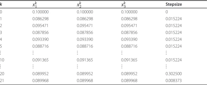
We applied MATLAB 7.0 to some problems of GNEPs. The method is terminated whenever ∥∇Ψ(ωk)∥<εwithε:= 10-7. The computational results are summarized in Tables 1, 2, and 3, which indicate that the proposed method produces good approxi-mate solutions.

Example 4.1 This test problem is the internet switching model introduced by Facchi-nei et al. [19].The payoff function of each user is given by

θν_{(x) :=} xν

B − xν $N

ν=1xν

,

with constraints xv≥0.01,ν= 1,...,N and#N ν=1x

ν _{≤B.According to[20],we also set}

N= 10,B= 1and use the starting pointx0_{=(0.1, 0.1, 0.1, ...,)}T_∈ 10_{. The exact} solu-tion of this problem is x* = (0.09,0.09,..., 0.09)T.We only state the first three components of the iteration vectors in Table 1.

Example 4.2This example is the river basin pollution game taken from[5]and is also

analyzed by Heusinger and Kanzow [20]. There are three players, each controlling a

single variablexν∈ .The objective functions are

θν_{(x) :=x}ν_c

1ν+c2νxν−d1+d2

x1+x2+x3

forν = 1,2,3,and the constraints are

μ11e1x1+μ21e2x2+μ31e3x3≤K1, μ12e1x1+μ22e2x2+μ32e3x3≤K2.

The economic constants d1 and d2 determine the inverse demand law and set to 3.0

and 0.01, respectively. Values for constants c1,v,c2,v,ev,μv,1andμV,2are given in the

fol-lowing table, and K1=K2 = 100. Table 2for the corresponding numerical results.

Table 1 Numerical results for Example 4.1

k xk1 xk2 xk3 Stepsize

0 0.100000 0.100000 0.100000 0

1 0.086298 0.086298 0.086298 0.015224

2 0.095471 0.095471 0.095471 0.015224

3 0.087856 0.087856 0.087856 0.015224

4 0.093390 0.093390 0.093390 0.015224

5 0.088716 0.088716 0.088716 0.015224

⋮ ⋮ ⋮ ⋮ ⋮

10 0.091365 0.091365 0.091365 0.015224

⋮ ⋮ ⋮ ⋮ ⋮

20 0.089952 0.089952 0.089952 0.302500

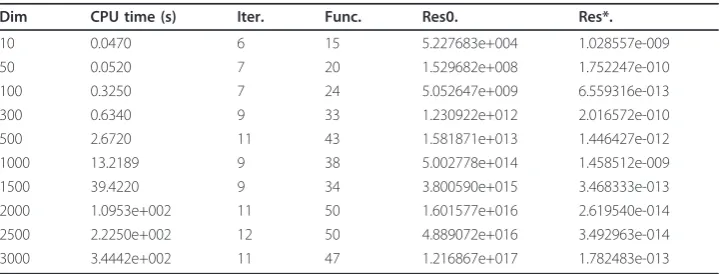
Example 4.3 We use Algorithm 4.1 to solve a class of problems in which for each playerν, his payoff functionθν(·) is quadratic, that is

θν_{(x) :=} 1

2

xνTA_ννxν+

N

#

μ=1,μ=ν

(xν)TA_νμxμ

for certain matrices A_νμ∈Rnν×_Rnμ_{such that the diagonal blockAννare symmetric.} Let

B:= ⎡ ⎢ ⎢ ⎢ ⎣

A11 A12 · · · A1N

A21 A22 · · · A2N

..

. ... . .. ... AN1AN2· · · ANN

⎤ ⎥ ⎥ ⎥ ⎦

be positive definite, The strategy spaceX is defined by some linear constraints. For convenience, we set the elements of x0 all 1. The elements of l0 all 0. We set other parameters in the algorithm as r = 10-8, = 2.1,s= 10-4,b = 0.55. Our numerical results are reported in Table 3, where Iter., Func, Res0. and Res*. stand for, respec-tively, the number of iterations, the number of function evaluations, the residual ∥∇Ψ(·)∥ at the starting point and the residual ∥∇Ψ(·)∥ at the final iterate of implementation.

Table 2 Numerical results for Example 4.2

k xk₁ xk₂ xk₃ Stepsize

0 0.000000 0.000000 0.000000 0.0000

1 9.208951 2.481282 8.931660 0.166375

2 11.531188 3.106991 11.183971 0.050328

3 12.744136 3.433811 12.360396 0.027680

4 13.100896 3.529937 12.706414 0.008373

5 13.159756 3.545796 12.763501 0.001393

6 13.177536 3.550587 12.780746 0.000421

7 13.182912 3.552036 12.785960 0.000127

8 21.175468 16.026854 2.771656 1

9 21.149274 16.027708 2.732634 1

10 21.144948 16.027849 2.726189 1

11 21.144796 16.027853 2.725963 1

Table 3 Numerical results for Example 4.3

Dim CPU time (s) Iter. Func. Res0. Res*.

10 0.0470 6 15 5.227683e+004 1.028557e-009

50 0.0520 7 20 1.529682e+008 1.752247e-010

100 0.3250 7 24 5.052647e+009 6.559316e-013

300 0.6340 9 33 1.230922e+012 2.016572e-010

500 2.6720 11 43 1.581871e+013 1.446427e-012

1000 13.2189 9 38 5.002778e+014 1.458512e-009

1500 39.4220 9 34 3.800590e+015 3.468333e-013

2000 1.0953e+002 11 50 1.601577e+016 2.619540e-014

2500 2.2250e+002 12 50 4.889072e+016 3.492963e-014

The numerical experiments show that the method proposed in this article is imple-mentable and effective.

Acknowledgements

The research was supported by the Fundamental Innovation Methods Funds under Project No. 2010IM020300 and the Technology Research of Inner Mongolia under Project No. 20100915.

Author details

1

Institute of ORCT, School of Mathematical Sciences, Dalian University of Technology, Dalian 116024, China 2_{Management College of Inner Mongolia University of Technology, Hohhot 010051, China}

Authors’contributions

JH and Z-CW carried out the design of the study and performed the analysis. ZW participated in its design and coordination. All authors read and approved the final manuscript.

Competing interests

The authors declare that they have no competing interests.

Received: 12 October 2011 Accepted: 9 March 2012 Published: 9 March 2012

References

1. Debreu, G: A social equilibrium existence theorem. Proc Natl Acad Sci USA.38, 886–893 (1952). doi:10.1073/ pnas.38.10.886

2. Altman, E, Wynter, L: Equilibrium, games, and pricing in transportation and telecommunication networks. Netw Spat Econ.4, 7_–21 (2004)

3. Hu, X, Ralph, D: Using EPECs to model bilevel games in restructured electricity markets with locational prices. Oper Res.

55, 809_–827 (2007). doi:10.1287/opre.1070.0431

4. Krawczyk, JB: Coupled constraint Nash equilibria in enviromental games. Resour Energy Econ.27, 157–181 (2005). doi:10.1016/j.reseneeco.2004.08.001

5. Krawczyk, JB, Uryasev, S: Relaxation algorithms to find Nash equilibria with economic applications. Environ Model Assess.5, 63–73 (2000). doi:10.1023/A:1019097208499

6. Uryasev, S, Rubinstein, RY: On relaxation algorithms in computation of noncoopera-tive equilibria. IEEE Trans Autom Control.39, 1263–1267 (1994). doi:10.1109/9.293193

7. Flam, SD, Ruszczynski, A: Noncooperative convex games: computing equilibrium by partial regulalization. IIASA Working Paper Austria. 94–142 (1994)

8. Gürkan, G, Pang, JS: Approximations of Nash equilibria. Math Program.117, 223_–253 (2009). doi:10.1007/s10107-007-0156-y

9. Heusinger, AV, Kanzow, C: Optimization reformulations of the generalized Nash equilibrium problem using Nikaido-Isoda-type functions. Comput Optim Appl.43, 353–377 (2009). doi:10.1007/s10589-007-9145-6

10. Facchinei, F, Pang, JS: Finite-dimensional variational inequalities and complementarity problems.I, Springer, New York (2003)

11. Facchinei, F, Pang, JS: Finite-dimensional variational inequalities and complementarity problems. Springer, New YorkII

(2003)

12. Harker, PT: Generalized Nash games and quasi-variational inequalities. Eur J Oper Res.54, 81–94 (1991). doi:10.1016/ 0377-2217(91)90325-P

13. Facchinei, F, Fisher, A, Piccialli, V: On generalized Nash games and variational inequalities. Oper Res Lett.35, 159–164 (2007). doi:10.1016/j.orl.2006.03.004

14. Qi, L: Convergence analysis of some algorithms for solving nonsmooth equations. Math Oper Res.18, 227–244 (1993). doi:10.1287/moor.18.1.227

15. Clarke, FH: Optimization and Nonsmooth Analysis. John Wiley, New York (1983)

16. Mifflin, R: Semismooth and semiconvex functions in constrained optimization. SIAM J Control Optim.15, 959–972 (1977). doi:10.1137/0315061

17. Qi, L, Sun, J: A nonsmooth version of Newton’s method. Math Program.58, 353–368 (1993). doi:10.1007/BF01581275 18. Luca, TD, Facchinei, F, Kanzow, C: A semismooth equation approach to the solution of nonlinear complementarity

problems. Math Program.75, 407–439 (1996)

19. Facchinei, F, Fisher, A, Piccialli, V: Generalized Nash equilibrium problems and Newton methods. Math Program.117, 163–194 (2009). doi:10.1007/s10107-007-0160-2

(Continued)

playerν c1,ν c2,ν ev μv,1 μv,2

1 0.10 0.01 0.50 6.5 4.583

2 0.12 0.05 0.25 5.0 6.250

20. Heusinger, AV, Kanzow, C: Relaxation methods for generalized Nash equilibrium problems with inexact line search. J Optim Theory Appl.143, 159_–183 (2009). doi:10.1007/s10957-009-9553-0

doi:10.1186/1029-242X-2012-60

Cite this article as:Houet al.:A variational inequality method for computing a normalized equilibrium in the generalized Nash game.Journal of Inequalities and Applications20122012:60.

Submit your manuscript to a

journal and benefi t from:

7Convenient online submission

7Rigorous peer review

7Immediate publication on acceptance

7Open access: articles freely available online

7High visibility within the fi eld

7Retaining the copyright to your article