THE RESEARCH AND APPLICATION OF CURVE AND
SURFACE FITTING PARALLEL LEAST SQUARES
ALGORITHM
1,2
YUZHU ZHANG, 1,2AIMIN YANG, 2YUE LONG
1
College of Mechanical Engineering, Yanshan University, Qinhuangdao 066004, Hebei, China 2
Hebei United University, Tangshan 063009, Hebei, China E-mail: 1aimin_heut@163.com
ABSTRACT
Along with the science research field is more and more wide, solve large-scale over determined system of linear equations has become an important problem , and the parallel processing technology also become the trend of the research. Firstly, this paper introduces the basic principle of the curve fitting least squares serial algorithm, based on the least square principle we found an parallel least squares curve and surface fitting method; Second, further reform the parallel least squares fitting method combined with parallel QR decomposition technique, which solved the problem of over determined linear equations and three dimensional space curved surface fitting. At the end of the paper we compared to scatter diagram and fitting chart with serial and parallel operation time which proves that the advantages and effectiveness of the method through the concrete example.
Keywords: Curve Fitting, Surface Fitting, Least Squares, Matrix Parallel Algorithms, Master-Slave Mode
1. INTRODUCTION
For a long time, the rapid development of parallel computer in order to improve the scientific compute speed, which makes the large science and engineering can be calculated and make scientific computing as a scientific research of three kinds of scientific method in scientific theory and scientific experiments [1-5]. And with the computer hardware, software and the progress of the algorithm produced, this trend become strengthens. With the increasing popularity of the high performance parallel machine, especially low price performance ratio of computer application and parallel programming standards, the high performance parallel computing has become a key supporting technology of China's science and engineering who want to apply the numerical simulation, and it is engaged in the science and engineering calculation of professional researchers or a foundation course that students want to study [6-11].
Least squares method is a kind of mathematical optimization technique. The basic idea is seeking for the best function matching data by minimize the sum of squares error. The fitting function method called the least squares fitting. Using least square
method can easily get unknown data, and make the solution has the minimum sums of squares error of obtained data and real data. The best matching function is called the least squares fitting function of the known data. Least squares fitting can be divided into linear least squares fitting and nonlinear least squares fitting [8-10].
ISSN: 1992-8645 www.jatit.org E-ISSN: 1817-3195
parallel algorithm in linear problem, Deren Wang puts forward some solutions to large linear problem parallel method according to matrix splitting technology, Zhong Chen analyzed the convergence of least squares parallel algorithm , but the basic is not involved in the curve fitting least squares acceleration ratio and efficiency analysis ,there is no design surface fitting least squares method. Based on the partition strategy and master-slave mode, with the parallel QR decomposition method, this paper studies the curved surface and curve fitting least squares algorithm, and finally gives the surface fitting example, this study provides a new method solution of over determined linear equations [5-9].
2. PARALLEL LEAST SQUARES
ALGORITHM
We mainly introduced the curve fitting least squares parallel algorithm design process, surface fitting problem can be finished after expanding.
Assume there is n dimension polynomial y=a0+a x1 +a x2 2+ + a xn n , the error is defined as:
2
0 1 2
n
i i i n
I = −Y y = −Y a −a x−a x − − a x
Among them, Yi is corresponding to the
observation or experimental data, which has free error, in order to solve the value in sum of squares of the minimum:
N
2 2 2
0 1 2
1 1
( )
N
n
i i i n i
i i
S I Y a a x a x a x
= =
=
∑
=∑
− − − − −In the minimum point, the partial derivative,
0
/ S a
∂ ∂ ,∂S/∂a1,, ∂S/∂anare zero. So we get
1
n+ equations:
(
)
( )
(
)
( )
(
)( )
2 0 1 0 1 2 0 1 1 1 2 0 1 10 2 1
0 2
0 2
N
i i i i
i
N
i i i i i
i
N
n
i i i i i
n i
S
Y a a x a x
a
S
Y a a x a x x
a
S
Y a a x a x x
a = = = ∂ = = − − − − − ∂ ∂ = = − − − − − ∂ ∂ = = − − − − − ∂
∑
∑
∑
Each equation both sides divided by -2 then we arranged to n+1 equations:
2
0 1 2
2 3 1
0 1 2
2 3 4 2 2
0 1 2
1 2 2
0 1 2
n
i i n i i
n
i i i n i i i
n
i i i n i i i
n n n n n
i i i n i i i
a N a x a x a x Y
a x a x a x a x x Y
a x a x a x a x x Y
a x a x a x a x x Y
+ + + + + + + + = + + + + = + + + + = + + + + =
∑
∑
∑
∑
∑
∑
∑
∑
∑
∑
∑
∑
∑
∑
∑
∑
∑
∑
∑
If these equations are written into matrix form, the all sum variables are from 1 toN.
2 3
2 3 4 1
2
2 3 4 5 2
1 2 3 2
n
i i i i i
n
i i
i i i i i
n
i i
i i i i i
n
n n n n n
i i
i i i i i
N x x x x Y
x Y x x x x x
a x Y x x x x x
x Y x x x x x
+ + + + + =
∑
∑
∑
∑
∑
∑
∑
∑
∑
∑
∑
∑
∑
∑
∑
∑
∑
∑
∑ ∑
∑
∑
∑
Coefficient matrix B is called formal matrix of the least squares problem. And the coefficient matrix B have more troublesome to calculating with
∑
, in order to reduce computation cost and complexity, we can use matrix parallel multiplication to elimination∑
then we can get simplified coefficient matrix *B .
We can find a matrix which is corresponding to coefficient matrixBand it is called design matrix [9]. It is form
1 2 3
2 2 2 2
1 2 3
1 2 3
1 1 1 1
N
N
n n n n
N
x x x x
A x x x x
x x x x
= 2
1 1 1
2
2 2 2
2
3 3 3
2 1 1 1 1 n n n n
N N N
x x x
x x x A x x x
x x x
Τ =
It is easy to be proved thatAAΤ =B, and Ayis
the right end vector; hereyis column vector which is consisting ofYi. It can be written as the following
form:
AA aΤ =Ay. We get evaluation *
to the line, then each piece contains
(
n+1)
p lines; The matrix AΤ is divided into ppieces according to the column, then each piece contains(
n+1)
p columns.When
(
n+1)
p is integer, Matrix parallel multiplication steps are as follows:First step: The first row of the matrix A multiplied with the matrix AΤ in each block column, according to the matrix multiplication, we can get numerical SolutionB∗of the first row can be obtained as B1,i
∗
(
i=1, 2 , 3,,n+1)
,Then each of the blocks in a row but the first row except of the matrix A respectively multiply with the first column of the matrix AΤ then the numerical solution B∗ of the first column asBi,1
∗
(
i=2 , 3, 4 ,,n+1)
。The second step: The second row of the matrixAare multiplied by the matrix AΤin each block column except the first column, according to the matrix multiplication we can get B∗of the rest
of the second line numerical solution of
2,i
B∗
(
i=2 , 3, 4 ,,n+1)
,Then the matrix A of rows in each block(except the first two lines)multiply with the second column of the matrixAΤ, according to the matrix multiplication we get theB∗of rest of the second column of the numerical solution Bi,2∗
(
i=3, 4 , 5,,n+1)
.
Following the steps of sequentially used the matrixAof the 3, 4 , 5,,n+1 line multiplied with the matrixAΤin each block column Then followed by the matrix Arows in each block respectively multiply with the 3, 4 , 5,,n+1 column of the
matrix AΤmultiplication, according to the matrix multiplication we finally obtained a simplified new coefficient matrix asB∗
1,1 1,2 1,3 1, 1
2,1 2,2 2,3 2, 1
3,1 3,2 3,3 3, 1
1,1 1,2 1,3 1, 1
n
n
n
n n n n n
b b b b
b b b b
B b b b b
b b b b
∗ ∗ ∗ ∗
+
∗ ∗ ∗ ∗
+
∗ ∗ ∗ ∗ ∗
+
∗ ∗ ∗ ∗
+ + + + +
=
Among them,bi j,
∗
as specific numerical values(
1, 2 , 3, , 1
i= n+ ; j=1, 2 , 3,,n+1)
When
(
n+1)
p is not integer ,(
n+1 / ()
p− =1) k mod q(
q< p)
,and satisfy with the following conditions(
p−1)
k+ = +q n 1, then the matrix A (and matrix AΤ ) Dividedinto p blocks by row (or column) , the1, 2 , 3,,p−1blocks has k row (or column), and the p blocks has q row (or column). Accordance with calculation method when
(
n+1)
p is integer, Sequentially used the matrix A of the 1, 2 , 3,,n+1 row respectively multiplied with the matrixAΤin each block column, The matrixAof rows in each block respectively multiplied with the matrix AΤ of the1, 2 , 3,,n+1 columns, then we can also be
obtained to simplify the coefficient matrix B∗. Throughout matrix multiplication parallel computing we can get the coefficient matrixB∗.
AA aΤ =Ay⇔B a∗ = Ay
The QR parallel processing on B∗ , then the
B∗will decomposed into orthogonal matrix and an upper triangular matrix plot. B∗ =QR, So make the general equation solving into triangular equations solving.
MatrixQRdecomposition can be used Givens
transform to achieve [6]. Standard Givens transform converting by selecting the appropriate plane of rotation the product QΤof the sequence to achieve, each transform eliminate an element under the main diagonal ofB∗without destroying the zero elements of the previously formed, So that Q BΤ ∗ =R. In order to eliminateB∗of
(
p q,)
non-zero elements, simply make the two linesp−1,p of B∗as thefollowing conversion:
1,1 1,2 1, 1,
,1 ,2 , ,
p p p q p n
p p p q p n
b b b b
c s
s c b b b b
− − − −
−
Among them, 2 , 2
, 1,
p q
p q p q
b s
b b −
=
+ ,
1,
2 2
, 1,
p q
p q p q
b c
b b
− −
=
+ and this permutation matrix is denoted as Gp q, ,so that the transformation B∗ of
ISSN: 1992-8645 www.jatit.org E-ISSN: 1817-3195
According to a column-by-column the Givens calculated as following Assume the matrix order number isn,if r=1, 2 , 3,,n−1,so
1
, 0
n r
r n i r
i
Q G
− − − =
= ∏ 1
0 r
r r i
i
B Q B
−
∗ ∗
− =
=
∏
Among them, Givens transform
(
)
, 1
p q
G ≤ < ≤q p n act on
1
, 1
1
p q
p i q q i
G B
− −
∗
− −
=
∏ two
linesp−1andp, erasing
(
p q,)
elements. Obviously we having(
n− +1) (
n− + + =2)
1 n n(
−1 2)
step-by-step transformation, we can get R B n 1∗ −
= ,
1 1
n
QΤ =Q− Q and this was Givens reduction process of matrixB∗.
Actually, the number of
(
p qk, k)
,(
)
1, 2, , 1 2
k= n n− in serial Givens reduction setS=
{
(
p q,)
1≤ < ≤q p n}
order by:( ) (
)
( ) ( ) (
)
( )
(
)
,1 , 1,1 , , 2,1 ; , 2 , 1, 2 , , 3, 2 ; ; , 1
n n n n
n n
− −
−
Among them
(
p qk, k)
expressed Givens transformG p q(
k, k)
role in(
k 1, k 1)
(
1, 1)
G p − q − G p q .B∗first two lines of
1
k
p− andpkeliminate the
(
p qk, k)
element.From the above-described serial algorithm can be seen the Givens reduction between zero suppression processes have strong constraints, however, some elements can still parallel zero suppression. Based on the correlation of Gp q, between each Givens
transform this paper give the QR orthogonal transformation of the fine-grained parallel algorithm. The rearrange the number in set, and divided them into different subsets Sr ,
1, 2 , 3, ,
r= l. Make them meet with
Sr =S,And each of the subset Sr in the rotation
transformation do not intersect with each other, but can execute in parallel. Their specific segmentation method as described as follow.
Parallel algorithm for elimination the element of
(
p q,)
, but not necessarily need to transform the role in the p−1, p line, Can act on any of the k line and pline(
k< p)
,only the k lineof
( )(
k j, 1≤ <j p)
elements is 0. So takeadvantage of this feature the number
(
p qk, k)
,(
)
1, 2 , 3, , 1 / 2
k= n n− on the
set S=
{
(
p q,)
1≤ < ≤q p n}
can decomposed asfollow :
First step: In the n,n/ 2 lines ; 1 / 2 1
n− ,n − lines ; ;n−n/ 2+1 1, givens transformation, to eliminate several elements at the following position at the same time:
(
n,1)
,(
n−1 1,)
, ,(
n−n/ 2+1 1,)
Obviously, above n/ 2Givens transforms do not intersect with each other.The second step: In then/ 2 ,n/ 4lines; ;
/ 2 / 4
n −k n −k
, lines ; ;
/ 2 / 4 1 1 n − n +
, lines ; n,n/ 2 + n/ 4 lines; ;n−k n, / 2 + n/ 4−k ; ;
/ 4 1 , / 2 1
n−n + n + Givens transformation, to eliminate several elements at the following position at the same time:
(
n/ 2,1)
(
n/ 2−1 1,)
,(
n/ 2 − n/ 4+1 1,)
(
n,2)
,(
n−1 2,)
,(
n−n/ 4+1 2)
, ,
Other steps empathy, calculated column Givens transform in turn. Taken=8for example; give the process of the Parallel Givens greedy algorithm
3
2 5
2 4 7
1 3 6 8
1 3 5 7 9
1 2 4 6 8 10
1 2 3 5 7 9 11
∗ ∗
∗ ∗
∗ ∗
∗ ∗
In processing resources unlimited case, above fine-grained parallel algorithms, each processor in each parallel step up to compute one Givens about andGp q, Qr only acting on the two rows ofQr ,
Other elements remain unchanged Two lines Gp q, B r
∗
corresponding to the participation B r
∗
sub-processor, each sub-processor is also required to pass the same result of the amount of data to the host processor So the total number of data transfer
(
1)
n n− times, the amount of data transfer
(
1 4)
n n− ⋅ n. Obviously, these fine-grained parallel algorithms for data transfer a large amount of O n
( )
3 , unsuitable for communication delay large cluster parallel computing systems, we should appropriate to improve the parallel algorithm the matrix QRdecomposition of coarse-grained parallel algorithm suitable for cluster systems.Network parallel computing environments to achieve parallel algorithm requires minimizing the communication overhead, and using the medium-grained task parallelism. To this end, according to the inherent parallelism of matrix QRfactorization, we redraw its task. Sub-blocks of the original matrix B∗ :Its rows and columns are divided into K equal parts, and these dividing lines intersect, the elements under the diagonal are divided into triangular sub-blocks or rectangular blocks, and then one of the rectangular sub-blocks in a diagonal line from left to right is divided into two triangular sub-block and the diagonal elements are contained in the in the lower right corner of the rectangular sub-blocks the sub-block. So we obtained 2
K triangular sub-blocks, The matrixB∗of theQR decomposition process actually
make the respective triangular sub-blocks of the elements into zero suppression, therefore each of which a triangular sub-block corresponding to the zero suppression task may be seen as a sub-task.
Obviously, we obtained 2
K triangular sub-blocks forB∗. Hutchison subtasks ifrom left to right in the j row block triangular corresponding to sub block i j,
T
(
1≤ ≤i K,1≤ ≤ −j 2i 1)
.According to the definition of Givens about, in the QR transformation process of the matrix B∗ Peer-element elimination process should column sequentially 1, 2,,n−1 and also asked if the elimination of the
(
p q,)
element, then asked participate in transformation of the first q−1element is 0 but q element was not. Therefore, the above task division obtained sub-tasks, The Givens transformations between the various sub-tasks and its internal elements should meet the following requirements:sub-tasks Ti j,
(
jmod 2=1)
,when Ti j, −1 hasbeen completed, it can only performed And if its corresponding block where the rectangular sub-block is viewed as theQRtransform matrix, Givens about of its internal elements is equivalent to the matrix, simply put the transformation matrix of the corresponding sub-blocks where the entire row block.
sub-tasks Ti j,
(
jmod 2=0)
,when i j, 1T − has been completed, it can only performed And its elements of Givens transformation requires the use of thekline block data, this need the line block to meet the subtasks k j, 1
T − have been executed, that its first triangular sub-blocks have been zero suppression.
Obviously, put matrix B∗ obtained into the division of sub-tasks, in each parallel steps, while satisfying with 1), 2) and has a plurality of parallel execution. This is the block parallel cluster system Givens reduction The matrix of rows and columns respectivelyKequal parts, Matrix diagonal Givens about elements are divided into 2
K triangular sub-blocks, Each triangular sub-block corresponds to a sub-task mark in accordance with the method described above In each of the parallel step, find all satisfy the conditions 1), 2) sub-tasks and assigned to each sub-processor parallel zero suppression.
According to the above-mentioned tasks, We can obtain the precursors of task graph, Scheduling algorithm is applied to the task pool can be obtained by the network parallel computing the matrix QR factorization environment sub block parallel algorithms. Actually, the scheduling procedure is a simple, The Intuitive approach is these subtasks to be seen as an element in the matrix, and applied the greedy algorithm on it little improvement and obtained each sub-task scheduling order.
The paper give the least squares curve fitting problem parallelization, If the known data group is expanded to a three-dimensional data set putli =( ,x yi i)T replace xi,then we will get the
least squares surface fitting problem of parallel computing.
3. LEAST-SQUARES ALGORITHM IS
APPLIED PARALLEL SURFACE FITTING
ISSN: 1992-8645 www.jatit.org E-ISSN: 1817-3195
based on least squares parallel algorithm design surface fitting. This method makes full use of the parallel features of the method of least squares, and it is able to maintain the image surface fitting results in the higher fitting accuracy premise so this fitting results facilitate has the efficient calculation of the surface characteristics of the depth image. By use the real depth image numerical experiments, the results illustrate is the effectiveness of the method.
There are two types of methods to calculate the curvature of the image surface, One is the use of differential geometry formulas calculated directly, since the direct calculation of the error is large, that has been rarely used. The other is Surface Fitting but this method within the local region on the image surface fitting, this method for some depth image complex area can not be well fitted in a short period of time.
To 1000Mbps Ethernet cluster simulation algorithm, the program uses the master-slave mode structure use the MPI + FORTRAN language and its implementation. 4-node cluster system design parallels least squares surface fitting algorithm simulation, assuming solving the QR decomposition is divided into four sub-tasks.
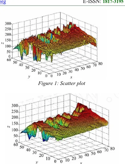
[image:6.612.315.523.79.353.2]To illustrate the effectiveness of the algorithm, experimental use of an image in the depth image library of the University of South Florida, as shown in Figure 1. In calculation process, all known data points either as a data point can be used as computing nodes, however, in the actual calculation process, we not used all the data points as compute nodes , but the depth of the image data, to trap a take one or the interval of two to take a as compute nodes. Such as compute nodes spaced points, the shape function through the compute nodes, and reuse all the data points of the depth image obtained after fitting the image surface. This not only can reduce the amount of computation, but can effectively reduce the random noise of the depth of the image itself. Compare via serial (see Figure 2) and parallel (Figure 3) algorithm fitting results visible, the fitting surfaces results are consistent But the use of the design of parallel algorithms for the 9.62s, far lower than that of the serial algorithm 27.68s so it has higher speedup and efficiency.
[image:6.612.327.511.378.490.2]Figure 1: Scatter plot
Figure 2: Serial fitting graphics (computing time 27.68s)
Figure 3: Parallel fitting graphics (computing time 9.62s)
A
CKNOWLEDGEMENTSThis work was supported by the National Natural Science Foundation of China (No. 51274270), Key Basic Research Project of Science and Technology Department of Hebei Province (No.10965633D) and the National Natural Science Foundation of Hebei Province (No. E2013209123).
REFERENCES:
[1] Curtis F.Gerald etc, “Numerical Analysis (version 7of the original book)”,beijing: Machinery Industry Press, Vol.69, 2006, pp.6-7.
Technology Press, Vol.45, 1989, pp.12-16. [3] Jiala Duo etc, “Summary of parallel
computing”,Beijing: Electronic Industry Press, Vol.65, 2004,pp.9-15.
[4] Guoliang Chen, “Parallel Computing - structure algorithm programming( revised version)”,Beijing: Higher Education Press, Vol.98, 2003, pp.3-6.
[5] Xavier (USA) Garr, “Introduction to Algorithms of Parallel”,Beijing: Machinery Industry Press, Vol.102, 2004, pp.4-5.
[6] Shixin Sun etc, “Parallel algorithm and its application”, Beijing: Machinery Industry Press, Vol.22, 2005, pp.61-66.
[7] John H,MathewsKurtis D.Fink,
“Numerical Methods Using MATLAB Fourth E dition”, Beijing:Electronic Industry Press, Vol.201, 2005, pp.10-15.
[8] G.H.Golub, D.F.Van Loan, “Matrix calculation”,DaLian: Dalian University of Technology Press, Vol.95, 1988, pp.12-18. [9] P.G.Ciarlet, “Matrix numerical analysis and
optimization”, Beijing: Higher Education Press, 1990, pp.18-21.
[10] Goodrich, “ Algorithm Analysis and Design”,
Beijing: People's Posts and
Telecommunications Press ,2006, pp.23-24. [11] Li Xie,Peng Wang, “Packaging
Engineering”,Beijing: Fifty-nine Institute of China Ordnance Industry, Vol.714, 2012, pp.13-15.
AUTHOR PROFILES:
Dr.Chunfeng Liu (1958- ), male.Professor in Yanshan University and Hebei United University. His research interests include numerical analysis, finite element method and parallel algorithms. Email: zyz@heuu.edu.cn
Aimin Yang (1978- ), male received the Master degree in Computational Math-ematics from Yanshan University in 2004. His interests are in data analysis and computational geometry.
He is a Associate Professor at Hebei United University. He has participated in several National Natural Science Fundation Projects and has hosted several Natural Science Foundation of Hebei Province and Educational Commission of Hebei Province of China.