ISSN: 1992-8645 www.jatit.org E-ISSN: 1817-3195
CONSTRUCTION OF AN OPTIMAL MATHEMATICAL
MODEL OF FUNCTIONING OF THE MANUFACTURING
INDUSTRY OF THE REPUBLIC OF KAZAKHSTAN
SEILKHAN N. BORANBAYEV, ASKAR B. NURBEKOV
L.N. Gumilyov Eurasian National University, Satpayev St., 2, Astana,010008, Kazakhstan
ABSTRACT
The article is devoted to the selection of an optimal model of the production function to simulate the functioning of the manufacturing industry of the Republic of Kazakhstan. An optimal model of the production function is selected from several models constructed and defined on the first stage of the study. The constructed optimal production function can be used to predict the value of gross domestic product based on the known or anticipated levels of capital and wage costs.
Keywords: model, method, simulation, forecasting, production function, capital.
1. INTRODUCTION
The condition and development of the manufacturing industry is one of the most important key points that determine the rate of economic development of the state.
As noted in the long-term strategy of development of Kazakhstan "Kazakhstan-2030", "the world experience shows the need for a specific progression, which consists in steady decline in the gross national product of the share of agriculture, mining, and, on the contrary, increase of the share of manufacturing industries and, above all, the science-intensive ones, with a high added value" [1].
Currently, the base materials sector is the basis of the Kazakhstan industry, which makes the state's economy dependent on the external factors such as demand and the level of prices for the exported raw materials. The raw material orientation dooms the state's economy to unequal foreign trade exchange and increasing technological inferiority.
In connection with this, the development of the manufacturing sector is of particular importance for the economic development of the Republic of Kazakhstan in modern conditions, and it was put in the foundation of the state Strategy of industrial-innovative development.
The production of competitive and export-oriented production in the manufacturing industry is the main concern of the state's industrial-innovation policy.
Due to the importance of manufacturing industry to the economy of Kazakhstan, it is necessary to use mathematical methods to forecast the industry’s development. This has defined the purpose and scope of our research. In the present paper, we use production functions to address this goal. Several production functions are constructed, and then an optimal model of the production function is chosen to forecast the development of the manufacturing industry of Kazakhstan.
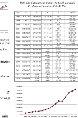
[image:1.612.313.522.588.727.2]For the mathematical simulation of the functioning of the manufacturing industry of the Republic of Kazakhstan, we use the data on the gross domestic product of this industry for 16 years (1998-2013) with respect to the labor force (L) and capital (K). The data are listed in Table 1 [2].
Table 1. The Economic Performance Of The Manufacturing Industry Of The Republic Of Kazakhstan
In The Years 1998-2013
Years K is the
capital costs (millions of
KZT)
L is the wage costs (millions of
KZT)
Y is the gross domestic product
of the industry (millions of
KZT)
1998 40 618.00 102 893.40 208 336.60
1999 52 907.28 130 240.20 284 152.00
2000 74 794.93 149 259.00 428 932.70
2001 102 421.81 167 483.10 534 563.00
2002 102 550.03 172 655.70 547 414.10
2003 119 870.48 213 417.00 655 719.00
2004 191 366.17 272 891.30 781 558.70
ISSN: 1992-8645 www.jatit.org E-ISSN: 1817-3195
Years K is the
capital costs (millions of
KZT)
L is the wage costs (millions of
KZT)
Y is the gross domestic product
of the industry (millions of
KZT)
2006 293 475.13 423 004.30 1 188 108.00
2007 316 339.43 551 380.20 1 476 647.60
2008 370 062.97 669 651.40 1 890 053.00
2009 396 261.47 643 251.10 1 849 097.50
2010 404 925.35 821 158.50 2 469 804.10
2011 455 466.43 989 957.40 3 131 187.00
2012 595 214.22 1 066 127.50 3 436 730.50
2013 636 886.41 1 130 987.00 3 651 704.60
2. TECHNIQUE
The methodological basis of the study is the works by the Russian and foreign scientists, the applied and theoretical works on economic-mathematical methods by Berezhnaya E.V and Berezhnoi V.I. [4], Granberg A.G. [5], Ivanilov Yu.P. [6], Malykhin V.I. [7], Rayatskas R.L. and Plakunov M.K. [8], Bagrinovsky K. A. and Matyushok V.M. [9], Solow R.M. [10], Gale D. [11], Dorfman R. [12], Cantor D.G. and Lipman S.A. [13], [14], Sonin I.M. [15], Presman E.L. and Sonin I.M. [16], on forecasting the economic data by Demidenko E.Z. [17], Dubrova T.A. [18], on the construction of production functions by Barkalov N.B. [19], Kleiner G.B. [20], and Nazarova N.V. [21].
The study is based on using the methods of mathematical simulation, system analysis, regression analysis, and others. The information base for the study includes the legislative and regulatory acts of the Republic of Kazakhstan, the materials of the Statistics Agency of the Republic of Kazakhstan and scientific publications.
3. RESULTS
3.1 Construction of a linear production function
Let us carry out mathematical simulation of the functioning of the manufacturing industry of the Republic of Kazakhstan. To do this, we construct several production functions, and then perform a comparative analysis.
We use the following model of a linear production function:
L
a
K
a
a
F
=
0+
1+
2,
(1)
where K is the capital costs; L is the wage costs.
The residual function has the form:
[
]
2 1 0, , 1
2 2 1 0 1
2
min
)
(
а а a n
i
i i i
n
i
i
=
∑
Y
−
a
+
а
K
+
а
L
→
∑
= =ε
(2)
We perform the calculations using the data of Table 1. As a result, we find that the residual function attains its minimum at а0 = -0.00003; а1 = -0.857; а2 = 3.542.
With respect to our data, the model of a linear production function will have the form:
L
K
F
=
−
0
.
00003
−
0
.
857
+
3
.
542
(3)
Table 2. The Economic Indicators Of The Manufacturing Industry Of Kazakhstan In The Years 1998-2013 With The Calculations Using The Linear Production
Function
Year s
K L Y F (Y-F)2
1998 40 618.00 102 893.40 208 336.60 329 572.937 14 698 249 288.010 1999 52 907.28 130 240.20 284 152.00 415 885.287 17 353 658
889.240 2000 74 794.93 149 259.00 428 932.70 464 474.241 1 263 201 126.582 2001 102 421.81 167 483.10 534 563.00 505 327.933 854 689 137.359
2002 102 550.03 172 655.70 547 414.10 523 536.849 570 123 105.254
2003 119 870.48 213 417.00 655 719.00 653 043.174 7 160 045.851
2004 191 366.17 272 891.30 781 558.70 802 372.072 433 196 461.944
2005 258 886.78 325 058.20 914 013.20 929 229.922 231 548 618.604
2006 293 475.13 423 004.30 1 188 108.00
1 246 451.724
3 403 990 175.921 2007 316 339.43 551 380.20 1 476
647.60
1 681 493.409
41 961 805 501.088 2008 370 062.97 669 651.40 1 890
053.00
2 054 290.411
26 973 927 261.342 2009 396 261.47 643 251.10 1 849
097.50
1 938 330.692
7 962 562 494.886 2010 404 925.35 821 158.50 2 469
804.10
2 560 964.491
8 310 216 969.393 2011 455 466.43 989 957.40 3 131
187.00
3 115 434.875
248 129 452.271
2012 595 214.22 1 066
127.50 3 436 730.50
3 265 372.922
29 363 419 450.599
2013 636 886.41 1 130
987.00 3 651 704.60
3 459 344.262
37 002 499 625.557
ISSN: 1992-8645 www.jatit.org E-ISSN: 1817-3195
Figure 1. Graphical Representation Of The Calculation Results While Using The Linear Production Function. The Blue Line Represents The Real Values; The Red
Line, The Values Of The Model.
The analysis of the data in Table 2 and Figure 1 shows that the constructed model of the linear production function sufficiently accurately reflects the development trend of the real indicators in its first half of the time interval, whereas in the second half there are some discrepancies.
As a result of the conducted regression analysis of the data, we obtain the following values:
•determination coefficient – 0.9928;
•standard error – 101 796.94;
•sum of the squared deviations – 190 638 377 603.9.
3.2 Construction of a Cobb-Douglas production function with α+β=1
Let us construct a Cobb-Douglas production function of the form:
β α
L
AK
F
=
,(4)
where α+β=1, K is the capital costs, L is the wage costs.
The residual function has the form:
[
]
1 0 1
1
, 1
2 ) 1 ( 0
1 2
min
)
a
(
a a n
i
a i a i i
n
i
i
=
∑
Y
−
K
L
→
∑
=
−
=
ε
(5)
We perform calculations using the data of Table 1. As a result, we find that the residual function reaches minimum at а0 = 2.822; а1 = -0.139.
With respect to our data, the model of the Cobb—Douglas production function with α+β=1 will have the form:
139 . 1 139 . 0
822
.
2
K
L
F
=
−(6)
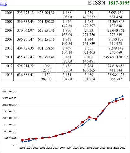
We perform calculations on the basis of the constructed production function. The calculation results are given in Table 3. Figure 2 provides a graphical representation of the results of calculations.
The analysis of the data of Table 3 and Figure 2 shows that the constructed model of the Cobb-Douglas production function with α + β = 1 behaves like the linear production function.
As a result of the conducted regression analysis of the data, we obtain the following values:
•determination coefficient – 0.9928;
•standard error – 101 445.767;
•sum of the squared deviations – 194 256 523 640.535.
Table 3. The Economic Indicators Of The Manufacturing Industry Of Kazakhstan In The Years 1998-2013 With The Calculations Using The Cobb-Douglas
Production Function With Α+Β=1
Years K L Y F (Y-F)2
1998 40 618.00 102
893.40 208 336.60
330 501.335 14 924 222 528.507
1999 52 907.28 130
240.20 284 152.00
416 675.887 17 562 580 615.467
2000 74 794.93 149
259.00 428 932.70
463 765.190 1 213 302
371.735
2001 102
421.81 167 483.10
534 563.00
506 154.948 807 017
432.710
2002 102
550.03 172 655.70
547 414.10
523 910.912 552 399
866.266
2003 119
870.48 213 417.00
655 719.00
652 658.144 9 368
841.680
2004 191
366.17 272 891.30
781 558.70
809 137.337 760 581
195.879
2005 258
886.78 325 058.20
914 013.20
946 882.238 1 080 373
680.083
2006 293
475.13 423 004.30
1 188 108.00
1 256 101.620
4 623 132 358.792
2007 316
339.43 551 380.20
1 476 647.60
1 681 217.991
41 849 045 075.867
2008 370
062.97 669 651.40
1 890 053.00
2 052 524.015
26 396 830 565.006
2009 396
261.47 643 251.10
1 849 097.50
1 942 004.301
8 631 673 689.999
2010 404
925.35 821 158.50
2 469 804.10
2 557 155.871
7 630 331 821.296
2011 455
466.43 989 957.40
3 131 187.00
3 112 717.883
341 108 265.066
2012 595
214.22 1 066 127.50
3 436 730.50
3 263 101.961
30 146 869 605.843
2013 636
886.41 1 130 987.00
3 651 704.60
3 457 468.440
[image:3.612.315.521.451.692.2]ISSN: 1992-8645 www.jatit.org E-ISSN: 1817-3195
Figure 2. Graphical Representation Of The Calculation Results By The Cobb-Douglas Production Function With
Α+Β=1.
The Blue Line Represents The Real Values; The Red Line, The Values Of The Model.
3.3 Construction of a Cobb-Douglas production function with α+β≠1
Let us construct a Cobb-Douglas production function of the form:
β α
L
AK
F
=
,(7)
where α+β≠1, K is the capital costs, L is the wage costs.
The residual function has the form:
[
]
2 1 0 2
1
, , 1
2 0
1 2
min
)
a
(
а a a n
i
a a i
n
i
i
=
∑
Y
−
K
L
→
∑
= =
ε
(8)
We perform calculations using the data of Table 1. As a result, we find that the residual function reaches minimum at а0 = 0.56; а1 = 0.004; а2 = 1.121.
With respect to our data, the model of the Cobb-Douglas production function with α+β≠1 will have the form:
121 . 1 004 . 0
56
.
0
K
L
F
=
(9)
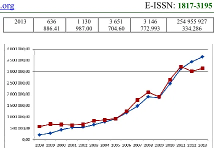
We perform calculations on the basis of the constructed production function. The calculation results are given in Table 4. Figure 2 provides a graphical representation of the results of calculations.
Table 4. The Economic Indicators Of The Manufacturing Industry Of Kazakhstan In The Years 1998-2013
With The Calculations Using The Cobb-Douglas Production Function With Α+Β≠1
Year s
K L Y F (Y-F)2
1998 40 618.00 102 893.40 208 336.60 242
870.986
1 192 623 841.205
1999 52 907.28 130 240.20 284 152.00 316
647.262
1 055 942 050.802
2000 74 794.93 149 259.00 428 932.70 369
432.548
3 540 268 146.566 2001 102 421.81 167 483.10 534 563.00 420
886.871
12 922 262 282.622 2002 102 550.03 172 655.70 547 414.10 435
487.283
12 527 612 263.155 2003 119 870.48 213 417.00 655 719.00 552
624.829
10 628 408 073.131 2004 191 366.17 272 891.30 781 558.70 729
324.344
2 728 427 932.668 2005 258 886.78 325 058.20 914 013.20 888
400.498
656 010 499.931
2006 293 475.13 423 004.30 1 188 108.00
1 194 119.445
36 137 474.474
2007 316 339.43 551 380.20 1 476 647.60
1 607 715.271
17 178 734 420.987 2008 370 062.97 669 651.40 1 890
053.00 2 000 274.026
12 148 674 668.573 2009 396 261.47 643 251.10 1 849
097.50 1 912 613.876
4 034 330 059.932 2010 404 925.35 821 158.50 2 469
804.10 2 515 010.202
2 043 591 669.680 2011 455 466.43 989 957.40 3 131
187.00 3 102 812.777
805 096 509.970
2012 595 214.22 1 066
127.50 3 436 730.50
3 375 271.455
3 777 214 208.153
2013 636 886.41 1 130
987.00 3 651 704.60
3 607 262.340
1 975 114 500.264
Figure 3. Graphical Representation Of The Calculation Results By The Cobb-Douglas Production Function For Α+Β≠1. The Blue Line Represents The Real Values; The
Red Line, The Values Of The Model.
Analysis of the data of Table 4 and Figure3 demonstrates that the constructed model of the Cobb-Douglas production function for α+β≠1 is sufficiently precise over the entire time interval under consideration.
As a result of the conducted regression analysis of the data, we obtain the following values:
• determination coefficient – 0.9959; • standard error – 76 549.895;
ISSN: 1992-8645 www.jatit.org E-ISSN: 1817-3195
3.4 Construction of a Cobb-Douglas production
function with α+β=1 taking into account scientific-technological progress (STP)
We will construct a Cobb-Douglas production function taking into account STP of the following form:
) 1 ( 0
α
−α
=
Ae
K
L
F
p t ,(10) where α+β=1, K is the capital costs, L is the
wage costs, t p
e
0is a special factor of scientific progress, p0 is a parameter of neutral STP (p0 > 0). The residual function has the form:
[
]
0 1 0 1
1 0
, , 1
2 ) 1 ( 0
1
2
(
a
)
min
p a a n
i
a a t p i
n
i
i
=
∑
Y
−
e
K
L
→
∑
=
−
=
ε
(11)
We perform calculations using the data of Table 1. As a result, we find that the residual function reaches minimum at p0 = 0.003; а0 = 2.833; a1 = -0.129.
With respect to our data, the model of the Cobb-Douglas production function with α+β=1 and taking into account STP will have the form:
129 . 1 129 . 0 003 . 0
833
.
2
e
K
L
F
=
t −(12) We perform calculations on the basis of the constructed production functions. The calculation results are given in Table 5. Figure 4 provides a graphical representation of the results of calculations.
Table 5. The Economic Indicators Of The Manufacturing Industry Of Kazakhstan For The Years 1998-2013
With The Calculations Using The Cobb-Douglas Production Function Taking Into Account STP With
Α+Β=1
Years K L Y F (Y-F)2
1998 40 618.00 102 893.40 208 336.60 329 491.108 14 678 414 848.254 1999 52 907.28 130 240.20 284 152.00 415 523.433 17 258 453
384.606 2000 74 794.93 149 259.00 428 932.70 463 472.106 1 192 970
592.786 2001 102 421.81 167 483.10 534 563.00 506 861.930 767 349 253.270
2002 102 550.03 172 655.70 547 414.10 524 486.900 525 656 478.339
2003 119 870.48 213 417.00 655 719.00 653 003.942 7 371 539.268
2004 191 366.17 272 891.30 781 558.70 811 397.852 890 374 963.193
2005 258 886.78 325 058.20 914 013.20 950 758.976 1 350 252 030.283
2006 293 475.13 423 004.30 1 188 108.00
1 259 473.537
5 093 039 881.424 2007 316 339.43 551 380.20 1 476
647.60
1 682 472.397
42 363 847 137.688 2008 370 062.97 669 651.40 1 890
053.00
2 053 271.756
26 640 362 273.849 2009 396 261.47 643 251.10 1 849
097.50
1 944 861.839
9 170 808 612.473 2010 404 925.35 821 158.50 2 469
804.10
2 555 121.403
7 279 042 247.669 2011 455 466.43 989 957.40 3 131
187.00
3 108 046.491
535 483 178.716
2012 595 214.22 1 066
127.50 3 436 730.50
3 264 630.365
29 618 456 411.584
2013 636 886.41 1 130
987.00 3 651 704.60
3 459 391.254
[image:5.612.312.522.77.324.2]36 984 423 065.707
Figure 4. Graphical Representation Of The Calculation Results By The Cobb-Douglas Production Function With
Taking Into Account STP And With Α+Β=1. The Blue Line Represents The Real Values; The Red Line, The
Values Of The Model.
Analysis of the data of Table 5 and Figure 4 shows that the constructed model of the Cobb-Douglas production function with α+β=1 and taking into account STP behaves analogously to the linear production function and the Cobb-Douglas production function without taking into account STP and with α+β=1.
As a result of the conducted regression analysis of the data, we obtain the following values:
• determination coefficient – 0.9929; • standard error – 101 087.447;
• sum of the squared deviations – 194 356 305 899.109.
3.5 Construction of a Cobb-Douglas production function taking into account scientific-technological progress (STP) with α+β≠1
We will construct a Cobb-Douglas production function taking into account STP of the following form:
β
α
L
K
Ae
F
=
p
0t
,
ISSN: 1992-8645 www.jatit.org E-ISSN: 1817-3195
where α+β≠1, K is the capital costs, L is the wage
costs, t p
e
0is a special factor of scientific progress, p0 is a parameter of neutral STP (p0 > 0). The residual function has the form:
[
]
2 0 1 0 2 1 0 , , , 1 2 0 1 2min
)
a
(
a p a a n i a a t p i n ii
=
∑
Y
−
e
K
L
→
∑
= =
ε
(14)
We perform calculations using the data of Table 1. As a result, we find that the residual function reaches minimum at p0 = 0.001; а0 = 29.985; а1 = -0.647; а2 = 1.45.
With respect to our data, the model of the Cobb-Douglas production function with α+β≠1 and taking into account STP will have the form:
45 . 1 647 . 0 001 . 0
985
.
29
e
K
L
F
=
t −(15)
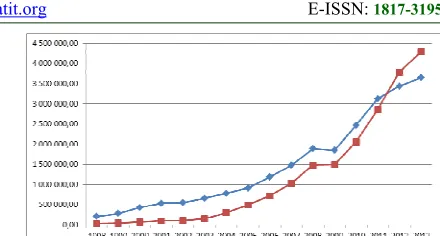
We perform calculations on the basis of the constructed production function. The calculation results are given in Table 6. Figure 5 provides a graphical representation of the results of calculations.
Table 6. The Economic Indicators Of The Manufacturing Industry Of Kazakhstan For The Years 1998-2013
With The Calculations Using The Cobb-Douglas Production Function Taking Into Account STP And With
Α+Β≠1
Years K L Y F (Y-F)2
1998 40 618.00 102
893.40 208 336.60
578 223.304
136 816 173 970.454
1999 52 907.28 130
240.20 284 152.00
685 808.539
161 327 975 681.466
2000 74 794.93 149
259.00 428 932.70
667 874.495
57 093 181 185.422
2001 102
421.81 167 483.10 534 563.00 643 953.838
11 966 355 466.617
2002 102
550.03 172 655.70 547 414.10 672 449.015
15 633 729 885.903
2003 119
870.48 213 417.00 655 719.00 826 533.490
29 177 590 044.496
2004 191
366.17 272 891.30 781 558.70 872 058.521
8 190 217 590.292
2005 258
886.78 325 058.20 914 013.20 924 144.032
102 633 754.371
2006 293
475.13 423 004.30 1 188 108.00 1 248 394.182
3 634 423 737.521
2007 316
339.43 551 380.20 1 476 647.60 1 746 537.908
72 840 778 282.891
2008 370
062.97 669 651.40 1 890 053.00 2 091 514.096
40 586 573 089.904
2009 396
261.47 643 251.10 1 849 097.50 1 887 536.871
1 477 585 249.085
2010 404
925.35 821 158.50 2 469 804.10 2 652 145.890
33 248 528 211.903
2011 455
466.43 989 957.40 3 131 187.00 3 223 007.497
8 431 003 621.479
2012 595
214.22 1 066 127.50 3 436 730.50 3 017 861.545
175 451 201 296.266
2013 636
886.41 1 130 987.00 3 651 704.60 3 146 772.993
[image:6.612.309.523.76.224.2]254 955 927 334.286
Figure 5. Graphical Representation Of The Calculation Results By The Cobb-Douglas Production Function With Taking Into Account Stp And With Α+Β≠1. The Blue Line Represents The Real Values; The Red Line, The Values
Of The Model.
Analysis of the data of Table 6 and Figure 5 shows that the obtained model of the Cobb-Douglas production function with α+β≠1 and taking into account STP does not reflect with sufficient precision the development tendency of the real indicators over the entire time interval under consideration.
As a result of the conducted regression analysis of the data, we obtain the following values:
• determination coefficient – 0.9729; • standard error – 196 752.076;
• sum of the squared deviations – 1 010 933 878 402.36.
3.6 Construction of a quadratic production function (of the type 1)
Let us construct a production function of the form: 2 4 2 3 2 1
0
a
K
a
L
а
K
a
L
a
F
=
+
+
+
+
(16)
where K is the capital costs, L is the wage costs. The residual function has the form:
[
]
4 3 2 1 0, , , , 1 2 2 i 4 2 i 3 i 2 i 1 0 1 2 min ) L K a L K a ( a a a a a n i i n i
i =
∑
Y− +a +a + +a →∑
= =ε
(17)
ISSN: 1992-8645 www.jatit.org E-ISSN: 1817-3195
As applied to our data, the model of a quadratic production function will have the form:
2 2
000002
.
0
000004
.
0
0007
.
0
00024
.
0
000000001
.
0
L
K
L
K
F
+
+
+
+
+
=
(18)
We perform calculations on the basis of the constructed production function. The calculation results are given in Table 7. Figure 6 gives a graphical representation of the calculation results.
Analysis of the data of Table 7 and Figure 6 shows that the obtained model of the quadratic production function (of the type 1) has substantial deviations from the real data over the entire time interval under consideration.
As a result of the conducted regression analysis of the data, we obtain the following values:
• determination coefficient – 0.9711; • standard error – 203 357.327;
[image:7.612.300.520.77.195.2]• sum of the squared deviations – 2 740 703 153 148.11.
Table 7. The Economic Indicators Of The Manufacturing Industry Of Kazakhstan In The Years 1998-2013 With The Calculations Using The Quadratic Production
Function (Of The Type 1)
Year s
K L Y F (Y-F)2
1998 40 618.00 102 893.40 208 336.60 28 574.908 32 314 266 075.165 1999 52 907.28 130 240.20 284 152.00 46 395.079 56 528 353
328.788 2000 74 794.93 149 259.00 428 932.70 68 791.645 129 701 579
478.189 2001 102 421.81 167 483.10 534 563.00 100 747.906 188 195 535
358.469 2002 102 550.03 172 655.70 547 414.10 104 469.337 196 200 062
995.551 2003 119 870.48 213 417.00 655 719.00 152 601.222 253 127 498
566.086 2004 191 366.17 272 891.30 781 558.70 303 327.690 228 704 899
146.879 2005 258 886.78 325 058.20 914 013.20 492 151.669 177 967 151
154.925 2006 293 475.13 423 004.30 1 188
108.00
720 972.195 218 215 860 213.761 2007 316 339.43 551 380.20 1 476
647.60
1 034 943.568
195 102 451 769.359 2008 370 062.97 669 651.40 1 890
053.00
1 482 685.732
165 948 090 711.226 2009 396 261.47 643 251.10 1 849
097.50
1 493 952.311
126 128 105 578.480 2010 404 925.35 821 158.50 2 469
804.10
2 057 117.740
170 310 031 680.475 2011 455 466.43 989 957.40 3 131
187.00
2 862 975.593
71 937 358 794.193 2012 595 214.22 1 066
127.50 3 436 730.50
3 787 001.194
122 689 559 324.952 2013 636 886.41 1 130
987.00 3 651 704.60
4 290 165.522
407 632 348 971.615
Figure 6. Graphical Representation Of The Calculation Results By The Quadratic Production Function. The Blue Line Represents The Real Values; The Red
Line, The Values Of The Model.
3.7 Construction of a quadratic production function (of the type 2)
Let us construct a production function of the form:
KL
a
L
a
K
а
L
a
K
a
a
F
=
0+
1+
2+
3 2+
4 2+
5(19)
where K is the capital costs, L is the wage costs. The residual function will have the following form:
[
]
5 4 3 2 1 0,, , , ,
1
2 5 2 i 4 2 i 3 i 2 i 1 0 1
2
min )
L K a L K a (
a a a a a a n
i
i i i
n
i
i =
∑
Y− +a +a + +a +aKL →∑
= =
ε
(20)
We carry out calculations using the data from Table 1. As a result, we get that the residual function attains minimum for а0 = 0; а1 = 0.000000000005; а2 = 0.000000000009; а3 = 0.0000015; а4 = 0.0000017; а5 = 0.0000021.
As applied to our data, the model of a quadratic production function will have the form:
KL L
K
L K
F
0000021 .
0 0000017 .
0 0000015 .
0
09 0000000000 .
0 05 0000000000 .
0 0
2 2
+ +
+
+ +
+ =
(21)
We perform calculations according to the constructed production functions. The calculation results are given in Table 8. Figure 7 gives a graphical representation of the calculation results.
[image:7.612.90.300.451.700.2]ISSN: 1992-8645 www.jatit.org E-ISSN: 1817-3195
With The Calculations Using The Quadratic Production Function (Of The Type 2)
Year s
K L Y F (Y-F)2
1998 40 618.00 102 893.40 208 336.60 28 989.956 32 165 218 547.263 1999 52 907.28 130 240.20 284 152.00 47 102.781 56 192 332
056.349 2000 74 794.93 149 259.00 428 932.70 69 328.773 129 314 984
013.043 2001 102 421.81 167 483.10 534 563.00 99 210.739 189 531 590
954.387 2002 102 550.03 172 655.70 547 414.10 103 342.241 197 199 816
163.244 2003 119 870.48 213 417.00 655 719.00 152 141.702 253 590 095
355.687 2004 191 366.17 272 891.30 781 558.70 291 156.503 240 494 315
181.738 2005 258 886.78 325 058.20 914 013.20 457 774.903 208 153 383
949.997 2006 293 475.13 423 004.30 1 188
108.00
693 856.927 244 284 122 833.111 2007 316 339.43 551 380.20 1 476
647.60 1 029 754.555
199 713 393 982.674 2008 370 062.97 669 651.40 1 890
053.00 1 482 287.359
166 272 818 298.918 2009 396 261.47 643 251.10 1 849
097.50 1 470 933.798
143 007 785 454.888 2010 404 925.35 821 158.50 2 469
804.10 2 078 634.309
153 013 805 014.998 2011 455 466.43 989 957.40 3 131
187.00 2 904 449.106
51 410 072 629.022 2012 595 214.22 1 066
127.50 3 436 730.50
3 781 906.838
119 146 704 508.309 2013 636 886.41 1 130
987.00 3 651 704.60
4 279 910.852
[image:8.612.91.298.122.494.2]394 643 094 916.688
Figure 7. Graphical Representation Of The Calculation Results By The Quadratic Production Function. The Blue Line Represents The Real Values; The Red
Line, The Values Of The Model.
Analysis of the data of Table 8 and Figure 7 yields the conclusion that the obtained model of the quadratic production function of the type 2, similar to the production function of the type 1, has substantial deviations from the real data over the entire considered interval of time.
As a result of the conducted regression analysis of the data, we obtain the following values:
• determination coefficient – 0.9722; • standard error – 199 632.8;
• sum of the squared deviations – 2 778 133 533 860.31.
3.8 Regression analysis of data
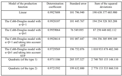
[image:8.612.312.522.198.329.2]Regression analysis of data was performed for each of the constructed production functions. The results of regression analysis of the data are shown in Table 9.
Table 9. The Results Of Regression Analysis Of The Data
Model of the production function
Determination coefficient
Standard error Sum of the squared deviations Linear 0.9927608 101 796.940 190 638 377 603.900 The Cobb-Douglas model with
α+β=1
0.9928107 101 445.767 194 254 528 383.208 The Cobb-Douglas model with
α+β≠1
0.9959064 76 549.895 87 250 448 602.112 The Cobb-Douglas model with
α+β=1 and taking into account STP
0.9928614 101 087.447 194 356 305 899.109 The Cobb-Douglas model with
α+β≠1 and taking into account STP
0.9729569 196 752.076 1 010 933 878 402.360 Quadratic (of the type 1) 0.9711106 203 357.327 2 740 703 153 148.110 Quadratic (of the type 2) 0.9721592 199 632.800 2 778 133 533 860.310
The criterion of selection is the following: maximum value of the determination coefficient, minimum error and minimum sum of the squared deviations.
As is seen from Table 9, the Cobb-Douglas production function with α+β≠1 fits the indicated selection criteria best of all. Besides, three models of the production function also satisfy the selection criteria:
• the linear one;
• the Cobb-Douglas one with α+β=1; • the Cobb-Douglas model with α+β=1 and with taking into account STP.
It is exactly these 4 models that will be considered on the second stage of choosing an optimal model.
3.9 Construction of additional models
The second stage of selecting an optimal model consists in constructing additional models based on the models selected on the first stage.
The algorithm for selection of an optimal model on the basis of an additional model is as follows:
• as the initial data there are taken the economic indicators of the manufacturing industry of Kazakhstan in the years 1998-2010;
• on the basis of these data, a corresponding additional model is constructed;
ISSN: 1992-8645 www.jatit.org E-ISSN: 1817-3195
2011-2013 on the basis of the known values of economic indicators K and L in the years 1998-2010;
• the real GDP values (Y) and the obtained values (F) of the additional model for the years 2011-2013 are compared.
Additional model of a linear production function
We will use a model of a linear production function
L
a
K
a
a
F
=
0+
1+
2 ,(22) where K is the capital costs, L is the wage costs.
The residual function has the form:
[
]
2 1 0, ,
1
2 2 1 0 1
2
min
)
(
а а a n
i
i i i
n
i
i
=
∑
Y
−
a
+
а
K
+
а
L
→
∑
= =
ε
(23) We carry out calculations using the data from Table 1. As a result, we get that the residual function attains minimum for а0 = -0.000009; а1 = -0.374; а2 = 3.087.
As applied to our data, the additional model of the production function will have the form:
L
K
F
=
−
0
.
000009
−
0
.
374
+
3
.
087
(24) In Table 10 there are presented the economic indicators of the manufacturing industry of Kazakhstan in the years 1998-2010 with additional calculations using the linear production function.
Table 10. Economic Indicators Of The Manufacturing Industry Of Kazakhstan In The Years 1998-2010
With Additional Calculations Using The Linear Production Function
Years K L Y F (Y-F)2
1998 40 618.00 102 893.40 208 336.60 302 422.628 8 852 180 695.121
1999 52 907.28 130 240.20 284 152.00 382 241.246 9 621 500 227.979
2000 74 794.93 149 259.00 428 932.70 432 763.575 14 675 604.602
2001 102 421.81 167 483.10 534 563.00 478 686.598 3 122 172 325.009
2002 102 550.03 172 655.70 547 414.10 494 605.461 2 788 752 317.633
2003 119 870.48 213 417.00 655 719.00 613 950.607 1 744 598 640.100
2004 191 366.17 272 891.30 781 558.70 770 799.990 115 749 846.853
2005 258 886.78 325 058.20 914 013.20 906 579.353 55 262 083.156
2006 293 475.13 423 004.30 1 188 108.00
1 195 985.448 62 054 186.578
2007 316 339.43 551 380.20 1 476 647.60
1 583 706.720 11 461 655 153.864
2008 370 062.97 669 651.40 1 890 053.00
1 928 696.739 1 493 338 569.457
2009 396 261.47 643 251.10 1 849 097.50
1 837 407.041 136 666 822.441
2010 404 925.35 821 158.50 2 469 804.10
2 383 332.782 7 477 288 861.870
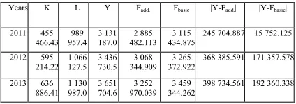
[image:9.612.312.524.443.518.2]On the basis of the data for K and L over the period 1998-2010, we calculate, using the additional model, the predicted values of F (Table 11). A graphical representation of the results of calculations by the linear production functions is given in Figure 8.
Figure 8. Graphical Representation Of The Calculation Results By The Linear Production Function. The Blue Line Represents The Real Values; The Red
Line, The Values Of The Model.
Table 11. Economic Indicators Of The Manufacturing Industry Of Kazakhstan In The Years 2011-2013
With Additional Calculations Using The Linear Production Function
Years K L Y Fadd. Fbasic |Y-Fadd.| |Y-Fbasic|
2011 455 466.43
989 957.4
3 131 187.0
2 885 482.113
3 115 434.875
245 704.887 15 752.125 2012 595
214.22 1 066 127.5
3 436 730.5
3 068 344.909
3 265 372.922
368 385.591 171 357.578 2013 636
886.41 1 130 987.0
3 651 704.6
3 252 970.039
3 459 344.262
398 734.561 192 360.338
Additional model of a Cobb-Douglas production function with α+β=1
Let us construct a Cobb-Douglas production function of the form:
β α
L
AK
F
=
,(25) where α+β=1, K is the capital costs, L is the wage costs.
The residual function has the form:
[
]
1 0 1
1
, 1
2 ) 1 ( 0
1 2
min
)
a
(
a a n
i
a i a i i
n
i
i
=
∑
Y
−
K
L
→
∑
=
− =
ε
ISSN: 1992-8645 www.jatit.org E-ISSN: 1817-3195
We carry out calculations using the data from Table 1. As a result, we get that the residual function attains minimum at а0 = 2.756; а1 = -0.072.
As applied to our data, the additional model of the linear production function will have the form:
072 . 1 072 . 0
756
.
2
K
L
F
=
−(27) In Table 12 there are presented the economic indicators of the manufacturing industry of Kazakhstan in the years 1998-2010 with additional calculations using the Cobb-Douglas production function for α+β=1.
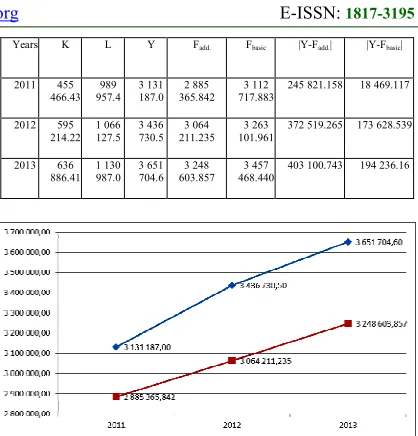
[image:10.612.314.523.75.293.2]On the basis of the data for K and L over the period 1998-2010, we calculate, using the additional model, the predicted values of F (Table 13). A graphical representation of the results of calculations by the Cobb-Douglas production function with α+β=1 is given in Figure 9.
Table 12. Economic Indicators Of The Manufacturing Industry Of Kazakhstan In The Years 1998-2010 With Additional Calculations Using The Cobb-Douglas
Production Function With Α+Β=1.
Year s
K L Y F (Y-F)2
1998 40 618.00 102 893.40 208 336.60 303 235.738
9 005 846 471.126 1999 52 907.28 130 240.20 284 152.00 383
035.100
9 777 867 556.019 2000 74 794.93 149 259.00 428 932.70 432
357.733
11 730 849.702 2001 102 421.81 167 483.10 534 563.00 478
212.158
3 175 417 386.146 2002 102 550.03 172 655.70 547 414.10 494
022.031
2 850 713 046.856 2003 119 870.48 213 417.00 655 719.00 613
125.263
1 814 226 427.390 2004 191 366.17 272 891.30 781 558.70 771
508.793
101 000 637.589 2005 258 886.78 325 058.20 914 013.20 910
575.884
11 815 139.734 2006 293 475.13 423 004.30 1 188
108.00 1 196 828.944
76 054 868.487 2007 316 339.43 551 380.20 1 476
647.60 1 581 629.847
11 021 272 088.434 2008 370 062.97 669 651.40 1 890
053.00 1 926 101.397
1 299 486 916.572 2009 396 261.47 643 251.10 1 849
097.50 1 835 693.889
179 656 790.545 2010 404 925.35 821 158.50 2 469
804.10 2 381 412.360
[image:10.612.93.298.426.668.2]7 813 099 722.069
Table 13. Economic Indicators Of The Manufacturing Industry Of Kazakhstan In The Years 2011-2013 With Additional Calculations Using The Cobb-Douglas
Production Function With Α+Β=1
Years K L Y Fadd. Fbasic |Y-Fadd.| |Y-Fbasic|
2011 455 466.43
989 957.4
3 131 187.0
2 885 365.842
3 112 717.883
245 821.158 18 469.117
2012 595 214.22
1 066 127.5
3 436 730.5
3 064 211.235
3 263 101.961
372 519.265 173 628.539
2013 636 886.41
1 130 987.0
3 651 704.6
3 248 603.857
3 457 468.440
403 100.743 194 236.16
Figure 9. Graphical Representation Of The Calculation Results By The Cobb-Douglas Production Function With Α+Β=1. The Blue Line Represents The Real Values; The
Red Line, The Values Of The Model.
Additional model a Cobb-Douglas production function withα+β≠1.
Let us construct a Cobb-Douglas production function of the form:
β α
L
AK
F
=
,(28) where α+β≠1, K is the capital costs, L is the wage costs.
The residual function has the form:
[
]
2 1 0 2
1
, , 1
2 0
1 2
min
)
a
(
а a a n
i
a a i
n
i
i
=
∑
Y
−
K
L
→
∑
= =
ε
(29) We carry out calculations using the data from Table 1. As a result, we get that the residual function attains minimum at а0 = 1.923; а1 = -0.028; а2 = 1.057.
As applied to our data, the additional model of the linear production function will have the form:
057 . 1 028 . 0
923
.
1
K
L
F
=
− [image:10.612.315.518.512.551.2]ISSN: 1992-8645 www.jatit.org E-ISSN: 1817-3195
Table 14. Economic Indicators Of The Manufacturing Industry Of Kazakhstan In The Years 1998-2010 With Additional Calculations Using The Cobb-Douglas
Production Function With Α+Β≠1.
Years K L Y F (Y-F)2
1998 40 618.00 102 893.40 208 336.60 283 976.384
5 721 376 885.953 1999 52 907.28 130 240.20 284 152.00 361
631.670
6 003 099 255.927 2000 74 794.93 149 259.00 428 932.70 413
645.831
233 688 360.711 2001 102 421.81 167 483.10 534 563.00 463
116.560
5 104 593 804.662 2002 102 550.03 172 655.70 547 414.10 478
232.474
4 786 097 365.138 2003 119 870.48 213 417.00 655 719.00 595
720.646
3 599 802 430.309 2004 191 366.17 272 891.30 781 558.70 762
440.689
365 498 362.247 2005 258 886.78 325 058.20 914 013.20 909
572.345
19 721 196.701 2006 293 475.13 423 004.30 1 188
108.00 1 197 358.976
85 580 554.741 2007 316 339.43 551 380.20 1 476
647.60 1 581 205.943
10 932 447 096.865 2008 370 062.97 669 651.40 1 890
053.00 1 933 281.785
1 868 727 848.512 2009 396 261.47 643 251.10 1 849
097.50 1 849 258.299
25 856.191
2010 404 925.35 821 158.50 2 469 804.10
2 392 402.203
5 991 053 678.765
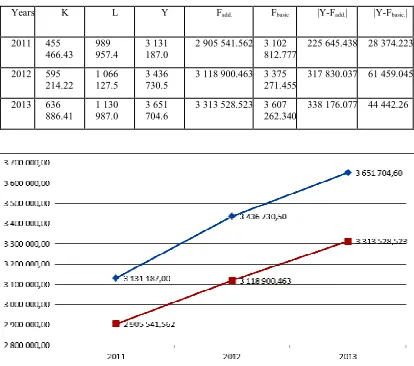
[image:11.612.315.523.319.357.2]On the basis of the data for K and L over the period 1998-2010 we calculate, using the additional model, the predicted values of F (Table 15). A graphical representation of the calculation results by the Cobb-Douglas production function with α+β≠1 is given in Figure 10.
Table 15. Economic Indicators Of The Manufacturing Industry Of Kazakhstan In The Years 2011-2013 With Additional Calculations Using The Cobb-Douglas
Production Function With Α+Β≠1
Years K L Y Fadd. Fbasic |Y-Fadd.| |Y-Fbasic.|
2011 455 466.43
989 957.4
3 131 187.0
2 905 541.562 3 102 812.777
225 645.438 28 374.223 2012 595
214.22 1 066 127.5
3 436 730.5
3 118 900.463 3 375 271.455
317 830.037 61 459.045 2013 636
886.41 1 130 987.0
3 651 704.6
3 313 528.523 3 607 262.340
338 176.077 44 442.26
Figure 10. Graphical Representation Of The Calculation Results By The Cobb-Douglas Production Function With
Α+Β≠1.
The Blue Line Represents The Real Values; The Red Line, The Values Of The Model.
Additional model of a Cobb-Douglas production function, taking into account STP, with α+β=1.
Let us construct a Cobb-Douglas production function, which takes into account STP, of the form:
) 1 ( 0
α
−α
=
Ae
K
L
F
p t ,(31)
where α+β=1, K is the capital costs, L is the wage
costs,
e
p0t is a special factor of scientific progress, p0 is a parameter of neutral STP (p0 > 0). The residual function has the form:[
]
0 1 0 1
1 0
, , 1
2 ) 1 ( 0
1
2
(
a
)
min
p a a n
i
a a t p i
n
i
i
=
∑
Y
−
e
K
L
→
∑
=
−
=
ε
(32)
We carry out calculations using the data from Table 1. As a result, we get that the residual function attains minimum at p0 = 0.0014; а0 = 2.752; а1 = -0.073.
As applied to our data, the additional model of the linear production function will have the form:
073 . 1 073 . 0 0014 . 0
752
.
2
e
K
L
F
=
t −(33)
In Table 16 there are presented the economic indicators of the manufacturing industry of Kazakhstan in the years 1998-2010 with additional calculations using the Cobb-Douglas production function with α+β =1 and with taking into account STP.
Table 16. Economic Indicators Of The Manufacturing Industry Of Kazakhstan In The Years 1998-2010 With Additional Calculations Using The Cobb-Douglas Production Function With Α+Β=1 And With Taking Into
Account STP.
Years K L Y F (Y-F)2
1998 40 618.00 102 893.40 208 336.60 303 484.036
9 053 034 597.986 1999 52 907.28 130 240.20 284 152.00 383
342.435
9 838 742 464.790 2000 74 794.93 149 259.00 428 932.70 432
652.493
[image:11.612.91.298.491.674.2]ISSN: 1992-8645 www.jatit.org E-ISSN: 1817-3195 2001 102 421.81 167 483.10 534 563.00 478
483.461
3 144 914 669.093 2002 102 550.03 172 655.70 547 414.10 494
310.582
2 819 983 676.471 2003 119 870.48 213 417.00 655 719.00 613
503.067
1 782 184 973.543 2004 191 366.17 272 891.30 781 558.70 771
885.814
93 564 726.972
2005 258 886.78 325 058.20 914 013.20 910 954.291
9 356 924.460
2006 293 475.13 423 004.30 1 188 108.00
1 197 421.171
86 735 153.451
2007 316 339.43 551 380.20 1 476 647.60
1 582 585.148
11 222 764 075.593 2008 370 062.97 669 651.40 1 890
053.00 1 927 306.230
1 387 803 153.460 2009 396 261.47 643 251.10 1 849
097.50 1 836 727.608
153 014 240.135
2010 404 925.35 821 158.50 2 469 804.10
2 383 057.893
7 524 904 489.558
[image:12.612.90.300.358.473.2]On the basis of the data for K and L over the period 1998-2010 we calculate, using the additional model, the predicted values of F (Table 17). A graphical representation of the calculation results by the Cobb-Douglas production function with α+β=1 and with taking into account STP is given in Figure 11.
Figure 11. Graphical Representation Of The Calculation Results By The Cobb-Douglas Production Function With Α+Β=1 And With Taking Into Account STP. The Blue
[image:12.612.312.523.414.510.2]Line Represents The Real Values; The Red Line, The Values Of The Model.
Table 17. Economic Indicators Of The Manufacturing Industry Of Kazakhstan In The Years 2011-2013 With Additional Calculations Using The Cobb-Douglas Production Function With Α+Β=1 And With Taking Into
Account STP
Years K L Y Fadd. Fbasic |Y-Fadd.| |Y-Fbasic|
2011 455 466.43
989 957.4
3 131 187.0
2 887 474.541
3 108 046.491
243 712.459 23 140.509
2012 595 214.22
1 066 127.5
3 436 730.5
3 066 110.001
3 264 630.365
370 620.499 172 100.135
2013 636 886.41
1 130 987.0
3 651 704.6
3 250 600.810
3 459 391.254
401 103.79 192 313.346
4. DISCUSSION
The Cobb-Douglas function is often used to simulate manufacturing. For example, in the paper
[22], by means of the Cobb-Douglas function, there is described the management of the production, which consumes a scarce natural resource and replaces outdated production assets. The model includes some resource-saving technological changes, various prices of resources and the ecological quotas of resource consumption. The model is reduced to nonlinear integral equations with unknown limits of integration. It is assumed in some models that the capital and resources are complementary factors of production [23, 25, 26, 27, 28]. Other models suggest that the capital and resource are interchangeable [24.31]. In the paper [30], it is demonstrated that the Cobb-Douglas function is the best for the problems with a non-renewable resource. A Cobb-Douglas function, involving capital and labor but without resource, is used in [29].
In our work we have carried out research and built some additional models of production functions in order to identify the optimal one for the manufacturing industry of Kazakhstan.
Let us bring together the results of constructing the additional models into a single table, Table 18.
Table 18. Indicators Of The Constructed Additional Models
Model of the production function
2011 2012 2013 Linear 2 885
482.113
3 068 344.909
3 252 970.039 The Cobb-Douglas model
with α+β=1
2 885 365.842
3 064 211.235
3 248 603.857 The Cobb-Douglas model
with α+β≠1
2 905 541.562
3 118 900.463
3 313 528.523 The Cobb-Douglas model
with α+β=1 and with taking into account STP
2 887 474.541
3 066 110.001
3 250 600.810 Real values 3 131 187 3 436 730.5 3 651 704.6
As is seen from Table 18, the data obtained by the Cobb-Douglas model of the production function with α+β≠1 are the closest ones to the real data. Thus, we select this model as an optimal one for the given industry.
5. CONCLUSION
The purpose of this paper is to construct an optimal mathematical model of functioning of the
manufacturing industry of the Republic of Kazakhstan. To solve this problem, there are created several models of production functions. Then, out of the constructed production functions, there is selected the optimal one for the
[image:12.612.92.300.601.703.2]ISSN: 1992-8645 www.jatit.org E-ISSN: 1817-3195
The selected optimal model of the Cobb-Douglas production function with α + β ≠ 1 can be used to predict the values of the gross domestic product on the basis of known or anticipated levels of the capital and wage costs.
In the future, similar research can be carried out for other sectors of the economy of Kazakhstan. In this case, to automate the processing of large volume of information and to perform computing works, one can create a software package having graphical interface which constructs the production functions, defines their parameters, makes forecasts, draws the corresponding graphics, etc.
REFERENCES:
[1] Kazakhstan - 2030: A Message from the President to the people of Kazakhstan. (n.d.).
Retrieved May 25, 2015, from
http://www.akorda.kz/ru/page/kazakhstan-2030_1336650228.
[2] The site of the Agency of Statistics of the Republic of Kazakhstan. (n.d.). Retrieved May 25, 2015, from http://www.stat.gov.kz/.
[3] The site of the information-analytical system "Taldau" of the Agency of Statistics of the Republic of Kazakhstan. (n.d.). Retrieved May 25, 2015, from http://taldau.stat.kz/.
[4] Berezhnaya, E., & Berezhnoi, V. (2003). Mathematical methods of simulation of economic systems. Moscow: Finance and Statistics.
[5] Granberg, A. (2004). Fundamentals of the regional economy. Moscow: Higher School of Economics.
[6] Ivanilov, Yu. (1999). Mathematical models in economics. Moscow: Nauka.
[7] Malykhin, V. (1998). Mathematical simulation of economy. Moscow: URAO.
[8] Rayatskas, R., & Plakunov, M. (1987). Quantitative analysis in economics. Moscow: Nauka.
[9] Barginovsky, K., & Matyushonok, V. (1999). Economic-mathematical methods and models (microeconomics). Moscow: RUSN.
[10] Solow, R. (1963). Capital theory and the rate of return. Amsterdam: North Holland Press. [11] Gale, D. (1973). On the theory of interest. The
American Mathematical Monthly, 8(80), 853-868.
[12] Dorfman, R. (1981). The meaning of internal rates of return. J. of Finance, 5(36), 1011-1021. [13]Cantor, D., & Lipman, S. (1983). Investment
selection with imperfect capital markets. Econometrica, 4(51), 1121-1144.
[14]Cantor, D., & Lipman S. (1995). Optimal Investment Selection with a Multitude of Projects. Econometrica, 5(63), 1231-1240. [15]Sonin, I. (1995). Growth rate, internal rates of
return and turn pikes in an investment model. Economic theory, (5), 383-400.
[16] Presman, E., & Sonin, I. (2000). Growth rate, internal rates of return and financial bubbles. Moscow, CEMI Russian Academy of Sciences. [17] Demidenko, E. (1981). Linear and nonlinear
regression. Moscow: Nauka.
[18]Dubrova, T. (2003). Statistical methods of forecasting. Moscow: UNITY-DANA.
[19] Barkalov, N. (1981). Production functions in the models of economic growth. Moscow State University.
[20] Kleiner, G. (1986). Production functions: theory, methods, applications. Moscow: Finance and Statistics.
[21] Nazarova, N. (2004). Mathematical modeling of production functions with probabilistic parameters (pp. 90-102). Krasnoyarsk: TORRA. [22] Hritonenko, N., Yatsenko, Yu., &
Boranbayev S. (2015). Environmentally sustainable industrial modernization and resource consumption: is the Hotelling’s rule too steep? Applied Mathematical Modelling, (39), 4365-4377.
[23] Azomahou, T., Boucekkine R., & Nguyen-Van, P. (2012). Vintage capital and the diffusion of clean technologies. Int. J. Econ. Theory, (8), 277-300.
[24] Caputo, M.R.. (2011). A nearly complete test of a capital accumulating, vertically integrated, nonrenewable resource extracting theory of a competitive firm. Resour. Energy Econ. (33), 725-744.
[25] Hritonenko, N., & Yatsenko, Yu. (2006). Optimization of financial and energy structure of productive capital. IMA J. Manage. Math. (17), 245-255.
[26] Hotelling, H. (1931). The economics of exhaustible resources. J. Political Econ. (39), 137-175.
ISSN: 1992-8645 www.jatit.org E-ISSN: 1817-3195
[28] Jovanovic, B., & Tse, C.-Y. (2010). Entry and exit echoes. Rev. Econ. Dyn. (13), 514-536. [29] Yatsenko, Yu., & Hritonenko, N. (2007).
Network economics and optimal replacement of age-structured IT capital. Math. Methods Oper. Res. (65), 483-497.
[30] Dasgupta, P., & Heal, G. (1974). The optimal depletion of exhaustible resources. Rev. Econ. Stud. (41), 3-28.