https://doi.org/10.5194/hess-21-4301-2017 © Author(s) 2017. This work is distributed under the Creative Commons Attribution 3.0 License.
Effect of unrepresented model errors on estimated soil hydraulic
material properties
Stefan Jaumann1,2and Kurt Roth1,3
1Institute of Environmental Physics, Heidelberg University, Im Neuenheimer Feld 229, 69120 Heidelberg, Germany 2HGSMathComp, Heidelberg University, Im Neuenheimer Feld 205, 69120 Heidelberg, Germany
3Interdisciplinary Center for Scientific Computing, Heidelberg University, Im Neuenheimer Feld 205, 69120 Heidelberg, Germany
Correspondence to:Stefan Jaumann ([email protected])
Received: 25 February 2017 – Discussion started: 2 March 2017
Revised: 27 June 2017 – Accepted: 21 July 2017 – Published: 1 September 2017
Abstract.Unrepresented model errors influence the estima-tion of effective soil hydraulic material properties. As the required model complexity for a consistent description of the measurement data is application dependent and unknown a priori, we implemented a structural error analysis based on the inversion of increasingly complex models. We show that the method can indicate unrepresented model errors and quantify their effects on the resulting material properties. To this end, a complicated 2-D subsurface architecture (AS-SESS) was forced with a fluctuating groundwater table while time domain reflectometry (TDR) and hydraulic potential measurement devices monitored the hydraulic state. In this work, we analyze the quantitative effect of unrepresented (i) sensor position uncertainty, (ii) small scale-heterogeneity, and (iii) 2-D flow phenomena on estimated soil hydraulic material properties with a 1-D and a 2-D study. The results of these studies demonstrate three main points: (i) the fewer sensors are available per material, the larger is the effect of unrepresented model errors on the resulting material prop-erties. (ii) The 1-D study yields biased parameters due to unrepresented lateral flow. (iii) Representing and estimat-ing sensor positions as well as small-scale heterogeneity de-creased the mean absolute error of the volumetric water con-tent data by more than a factor of 2 to 0.004.
1 Introduction
recorded during a fluctuating groundwater table experiment. With increasing computational power in recent years, 1-D subsurface architectures were analyzed with ensemble-based parameter estimation methods reaching from Markov chain Monte Carlo (MCMC; e.g., Vrugt et al., 2008b; Scharnagl et al., 2011; Wöhling and Vrugt, 2011) and data assimilation (e.g., Wu and Margulis, 2011; Li and Ren, 2011; Erdal et al., 2014) to data-driven modeling (e.g., Over et al., 2015).
Most of these studies describe the given data with models chosen upfront with restricted complexity and a minimum number of parameters. If the models are too simple, critical uncertainties and processes may be neglected, leading to sub-optimal results. If the models are too complex, the resulting material properties are likely to be application dependent. In general, the required model complexity is unknown a priori (Vereecken et al., 2015). Quantitative learning about compli-cated systems is an iterative process (Gupta et al., 2008; Box et al., 2015). It starts from the current understanding of the system that is represented with a model (Clark et al., 2011; Gupta et al., 2012). The optimal experimental design is then based on the model and the resulting data are, figuratively speaking, the answer of reality to the questions asked through the experiment. Disagreement between the model and the data reveals incorrect understanding of the system. Conse-quently, the concepts, decisions, and hypotheses integrated into the model (including evaluation procedures of the data) and the data themselves are revised. If the model predicts the data accurately and precisely enough, the research objectives are expanded, such that the data cover a larger part of the state space. Ultimately, this iterative procedure leads to data covering the whole state space and a statistical model–data mismatch corresponding to the data error model. In general, such data are not available and the application merely re-quires a limited accuracy and precision. Hence, the crux is to determine the sufficient complexity of both the model and the data for the required accuracy and precision.
This problem can be quantified with a Bayesian total er-ror analysis (BATEA; Kavetski et al., 2002, 2006) investi-gating the total uncertainty space which includes uncertainty in the observed input and responses as well as uncertainty in the model hypothesis. However, this analysis is computa-tionally intensive if the number of uncertainties is large and required models may not be available, e.g., for hysteresis. For instance, Bauser et al. (2016) categorized the uncertainties a priori and estimated the most important ones along with ef-fective material properties using an ensemble Kalman filter (EnKF) aiming for a consistent representation of reality. The temporal fluctuation of the estimated hydraulic parameters was used to identify a situation in which the representation of the dynamics is inconsistent. Hence, measurement data ac-quired during this period of time were merely used for state estimation and excluded from parameter estimation to pre-vent the incorporation of uncertainties in the dynamics into the estimated parameters.
Table 1.The grain size distribution in percent by weight displays the different granularity of the materials A, B, and C of ASSESS (G. Schukraft, personal communication, Institute of Geography, Heidelberg University, 2010). Whereas the composition of the ma-terials B and C is similar, material A features a higher percentage of fine sand. Since the mechanical wet analysis is time-consuming and laborious, only material B was sampled twice. Thus, 80 g out of approximately 400 Mg were sampled. Due to rounding, the sum of the values is not always 100.
Grain size range A B1 B2 C
Gravel total 2–63 mm (%) 2 5 4 5
Sand total 63–2000 µm (%) 97 96 95 95
coarse 630-2000 µm (%) 10 24 20 17
medium 200–630 µm (%) 65 64 68 72
fine 63–200 µm (%) 22 8 7 6
Silt total 2 –63 µm (%) 0 0 0 0
Clay total <2 µm (%) 0 0 0 0
In this work, we change the perspective and associate the model with our quantitative understanding of reality that is tested against the given measurement data. To analyze the required model complexity, we prescribe temporally constant material properties, calculate the maximum likelihood of in-creasingly complex models and analyze the corresponding structural model–data mismatch. We show that this structural error analysis indicates limitations of these models and quan-tifies the effect of the respective unrepresented model errors on the inversely estimated material properties. Specifically, we analyze measurement data acquired at the test site (AS-SESS) while it as forced with a fluctuating groundwater table which ensures a high dynamical range of the hydraulic state. We set up a basic representation accounting for uncertain-ties of the hydraulic material properuncertain-ties and the forcing. Fol-lowing an uncertainty analysis, we additionally estimate the sensor position and small-scale heterogeneity. These increas-ingly complex models are applied to (i) three 1-D profiles in ASSESS with an increasing number of sensors per material and (ii) the full 2-D profile to additionally analyze the impli-cations of the restriction to a 1-D subsurface architecture and to few sensors per material.
2 Methods 2.1 ASSESS
Figure 1. View of ASSESS site with tensiometer access tube, weather station, and groundwater well along the left boundary. The jump in color reveals different sands that crop out at the surface (figure adapted from Jaumann, 2012).
gravel layer, a concrete layer confines the site. As the test site is built into a former fodder silo, a concrete L element serves as additional wall. In order to stabilize the material during the construction, it was compacted. In addition to the compaction interfaces shown in Fig. 2, ground-penetrating radar (GPR) measurements indicate even more compaction interfaces (Klenk et al., 2015, Figs. 1b and 6).
The test site is equipped with a weather station, a ten-siometer (UMS T4-191), and 32 soil temperature and TDR sensors. Each TDR sensor has three cylindrical rods (length: 0.20 m, diameter: 0.004 m) which are separated by 0.03 m. They are operated by a Campbell Scientific TDR100. 2.2 Representation
For representing the soil water dynamics in ASSESS during the experiment, we follow Bauser et al. (2016) and define the representation of a system as a set consisting of dynamics (mathematical description), subscale physics (material prop-erties), forcing (superscale physics), and states. The repre-sentation of the hydraulic system also comprises its imple-mentation. In order to separate the more general theoretical considerations from the application-dependent details, these are not directly given in this section but are gathered in Ap-pendix A1.
2.2.1 Dynamics
The Richards equation (Richards, 1931) is the standard model to describe soil water dynamics:
∂tθ− ∇ ·K(θ )[∇hm(θ )−ez]=0, (1) with the time t (s), volumetric water contentθ (−), matric headhm(m), unit vector inzdirectionezindicating the di-rection of gravity, soil water characteristic θ (hm), and hy-draulic conductivity functionK(θ ). The material properties
θ (hm)andK(θ )are required to solve this partial differential equation. Generally, these material properties are non-linear and vary over many orders of magnitude.
2.2.2 Subscale physics
We choose the Brooks–Corey parameterization (Brooks and Corey, 1966) for the soil water characteristicθ (hm), since it has been found to describe the materials in ASSESS well (Dagenbach et al., 2013). This parameterization has four pa-rameters: a scaling parameterh0(m)related to the air en-try pressure (h0<0 m), the saturated water contentθs(−), the residual water content θr(−), and a shape parameter λ (−)related to the pore size distribution (λ >0). In general,
θ (hm) shows hysteretic behavior (Topp and Miller, 1966). Neglecting hysteresis, the parameterization may be inverted forθr≤θ≤θs. This leads to
hm(θ )=h0 θ−θ
r θs−θr
−1/λ
. (2)
Inserting the Brooks–Corey parameterization into the hy-draulic conductivity model of Mualem (1976) yields the pa-rameterization
K(θ )=Ks θ−θ
r θs−θr
τ+2+2/λ
(3)
for the hydraulic conductivity function, whereKs(m s−1)is the saturated hydraulic conductivity andτ (−)a heuristic tor-tuosity factor.
Small-scale heterogeneities, i.e., the texture of the porous medium, can be represented with Miller scaling if the pore spaces at any two points are assumed geometrically simi-lar (Miller and Miller, 1956). Scaling the macroscopic ref-erence stateh∗m(θ ),K∗(θ )with a local ratio of characteris-tic lengthsξ (−), leads to locally scaled material functions (Roth, 1995):
hm(θ )=h∗m(θ )·ξ, K(θ )=K ∗
(θ )/ξ2. (4)
2.2.3 Forcing
The hydraulic state was forced with a fluctuating ground-water table by pumping ground-water in or out of a groundground-water well. The experiment was arranged in three different phases: (i) initial drainage phase, (ii) multistep imbibition phase, and (iii) multistep drainage phase. The detailed forcing is pre-sented in Table 2. Throughout the forcing, equilibration steps were included in between, such that the relaxation of the cap-illary fringe happened within the measurement volume of the TDR sensors where possible. We neglect evaporation in the following, since the experiment took place at the end of November and the weather was cloudy with 2–7◦C air tem-perature. The last precipitation was measured approximately 10 days before the experiment.
2.2.4 State
Position [m]
Position [m] -1.8
-1.6 -1.4 -1.2 -1 -0.8 -0.6 -0.4 -0.2 0
2 4 6 8 10 12 14 16 18
t
w
1
2 3
4 5 6 7
8 9
10
11
12 13 14 15 16 17 18
19 20 21
22 23 24 25
26 27 28 29 30 31 32 A
B
C
C
B
[image:4.612.127.468.68.202.2]A
Figure 2.ASSESS features an effective 2-D architecture with three different kinds of sand (A, B, and C). The hydraulic state can be manip-ulated with a groundwater well (white square, at 18.2 m) and is automatically monitored with 32 TDR sensors (dots) and one tensiometer (black square, at 4.0 m). The color of the dots associates some of the TDR sensors with different cases of the 1-D study discussed in Sect. 3.1. The gravel layer at the bottom of the site ensures a rapid water pressure distribution over the site. An L element (black polygon, at 0.4 m) and compaction interfaces (white lines) were introduced during the construction. Note the different scales on the horizontal and vertical axes.
-1.6 -1.4 -1.2 -1 -0.8 -0.6 -0.4 -0.2 0
12:00 16:00 20:00 00:00 04:00 08:00 12:00 16:00 20:00 00:00 04:00
Position [m]
Time [hh:mm] (UTC)
Tensiometer Groundwater well
Figure 3.The position of the groundwater table was measured manually in the groundwater well and automatically with the tensiometer (Fig. 2) during three different phases (initial drainage, multistep imbibition, and multistep drainage – separated by the vertical black lines in the figure) of the experiment. Note that the discrete measurement steps reflect the resolution of the tensiometer.
experiment. The hydraulic potential was assessed via the po-sition of the fluctuating groundwater table. This popo-sition was measured (i) manually in the groundwater well and (ii) au-tomatically with the tensiometer (Fig. 3). The gradient be-tween the hydraulic potential in the groundwater well and the hydraulic potential in the test site drives the water flux. The largest part of this gradient equilibrates approximately within 5 min. Afterwards, the position of the groundwater table still changes due to the long-term equilibration of the hydraulic state.
The water content data are based on measured TDR traces which yield the relative permittivity of the soil εb (Sect. A1.3). This permittivity is converted to water contentθ
using the Complex Refractive Index Model (CRIM; Birchak et al., 1974):
εb(θ, T , φ)α=θ·εw(T )α+(φ−θ )·εαa+(1−φ)·εαs, (5) with the geometry parameter α=0.5. In order to apply the CRIM, the porosity φ, the relative permittivity of waterεw,
the relative permittivity of airεa, and the relative permittivity of the soil matrixεshave to be known. The relative permit-tivity of airεawas set to 1.0. Assuming that the sand matrix consists mainly of quartz (SiO2) grains, the relative permit-tivity of the soil matrixεswas set to 5.0 (Carmichael, 1989). Core samples of the materials A, B, and C yielded the porosi-ties 0.41, 0.36, and 0.38, respectively. These values will be assumed for the saturated water contentθsof the respective materials in the remainder of this paper. Following Kaatze (1989), we parameterize the dependency of the relative per-mittivity of waterεwon the soil temperatureT (◦C) with εw(T )=10.01.94404−T·1.991·10
−3
(6) and use soil temperature measurements near each TDR sen-sor to determine the accordingεw.
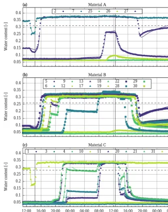
[image:4.612.126.467.284.420.2]0.05 0.1 0.15 0.2 0.25 0.3 0.35 0.4
(a)
(b)
(c)
Water content [-]
Material A
2 7 25 26 27
0.05 0.1 0.15 0.2 0.25 0.3 0.35 0.4
(a)
(b)
(c)
Water content [-]
Material B 5
6
9 12
13 17
18 19
22 28
29 30
0.05 0.1 0.15 0.2 0.25 0.3 0.35 0.4
12:00 16:00 20:00 00:00 04:00 08:00 12:00 16:00 20:00 00:00 04:00 (a)
(b)
(c)
Water content [-]
Time [hh:mm] (UTC) Material C
[image:5.612.125.463.65.490.2]1 3 4 10 11 20 21 31
Figure 4.The measured water content data for the three different phases (initial drainage, multistep imbibition, and multistep drainage – separated by the solid vertical black lines in the figure) show a high variability up to and beyond the validity limits of the Richards equation due to the fluctuating groundwater table (Fig. 3). Hence, in order to avoid effects related to entrapped air and two-phase flow phenomena, we neglect all data with a volumetric air content smaller than 0.1 (all values above the dashed horizontal lines) based on measured porosities from core samples. The colored solid lines show the results of the Miller and position setup of the 2-D study (Sect. 3.2). The data measured before 12:50 UTC are only used for the initial state estimation (Sect. A1.6).
creases quickly during the imbibition steps as the groundwa-ter table reaches the TDR sensor because of the narrow tran-sition zone of sandy materials during imbibition (Dagenbach et al., 2013; Klenk et al., 2015) and the small measurement volume of the TDR sensors (Robinson et al., 2003). During the equilibration phases, for example, after the last drainage phase (19:15 UTC), the measured water content in the unsat-urated material either decreases (e.g., sensor 27) or increases (e.g., sensor 2), depending on the hydraulic state at this posi-tion with respect to static hydraulic equilibrium. This effect is used in the following evaluation (Sect. 3.1.3).
We attribute the spread of the water content during satura-tion mainly to small-scale heterogeneity and quasi-saturasatura-tion due to entrapped air (Christiansen, 1944). In order to avoid effects related to entrapped air and also two-phase flow, all TDR data with an air content below 0.1 (Faybishenko, 1995) are neglected subsequently.
2.3 Structural error analysis
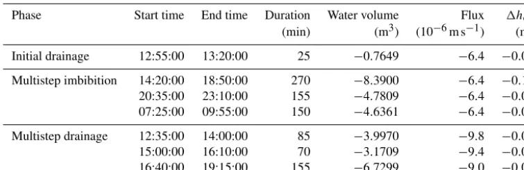
represen-Table 2.During the experiment, ASSESS was forced with a fluctuating groundwater table. Therefore, 17.8 m3of water were pumped in and 14.7 m3were pumped out of the groundwater well. For the calculation of the according flux and equivalent height of the water column1heq, the surface area of ASSESS was approximated with 80 m2. All times are given in UTC.
Phase Start time End time Duration Water volume Flux 1heq
(min) (m3) (10−6m s−1) (m)
Initial drainage 12:55:00 13:20:00 25 −0.7649 −6.4 −0.01
Multistep imbibition 14:20:00 18:50:00 270 −8.3900 −6.4 −0.10
20:35:00 23:10:00 155 −4.7809 −6.4 −0.06
07:25:00 09:55:00 150 −4.6361 −6.4 −0.06
Multistep drainage 12:35:00 14:00:00 85 −3.9970 −9.8 −0.05 15:00:00 16:10:00 70 −3.1709 −9.4 −0.04 16:40:00 19:15:00 155 −6.7299 −9.0 −0.08
tation errors. Some of those representation errors are param-eterized and included in the parameter estimation process. This allows to set up a number of distinct representations with increasing complexity. Using inversion to estimate op-timal parameters for each of these representations facilitates analyzing (i) the resulting residuals to improve the represen-tations and (ii) the effect of unrepresented model errors on the resulting material properties.
Preparing the tools for the method, we start this sec-tion with the Levenberg–Marquardt algorithm (Sect. 2.3.1) and discuss the assessment of the representation errors (Sect. 2.3.2) as well as the analysis of the resulting residu-als (Sect. 2.3.3) afterwards.
2.3.1 Levenberg–Marquardt
We employ the Levenberg–Marquardt algorithm for parame-ter estimation. Our implementation is based on Moré (1978), Press (2007), and Transtrum and Sethna (2012) together with some further modifications.
Assuming (i)Mdata pointsmµ(1, . . ., M) measured at po-sitionxµfeaturing a white Gaussian measurement error with standard deviationσµand (ii) a modelf withP parameters
pπ(1, . . ., P), theχ2cost function is defined as
χ2(p)=1
2 M
X
µ=1
m
µ−f (xµ,p)
σµ
2
=1
2 M
X
µ=1
rµ(p)2. (7)
This cost function assumes statistically independent residu-alsrµthat are normally distributed with zero mean and stan-dard deviationsσµ(perfect model assumption). These resid-uals can be expanded as
rµ(p+δp)≈rµ(p)+ P
X
π=1
Jµπδpπ (8)
with the Jacobi matrix Jµπ=∂rµ/∂pπ. The Jacobi matrix is assembled numerically with the finite differences method. Following Press (2007), the Hessian is approximated (H≈
J>J), assuming that the second term in the derivative cancels out as f (xµ,p)→mµ with an increasing number of iter-ations. Hence, for the Gauss–Newton algorithm, it follows that
δp= −(J>J)−1· ∇χ2(p). (9) SinceJ>Jdoes not always have full rank, the inversion may be ill-conditioned, leading to uncontrolled large steps. One possibility to cope with this issue is to regularize J>J by adding a diagonal damping matrixD>D.
We follow Transtrum and Sethna (2012) and choose this damping matrix, such that the diagonal entry forpπcontains the corresponding maximal diagonal entry ofJ>J from all
previous iterations if this value is larger than a predefined minimal value (1.0) which is used otherwise. The resulting damping matrix is scaled with a parameter λ which tunes both the amount of regularization and the step size of the parameter update.
Finally, the parameter updateδpis calculated via
δp= −(J>J+λ·D>D)−1· ∇χ2(p), (10) where the linear problem is solved with a singular value de-composition (SVD). If the condition number of the sensitiv-ity matrixS=J>J+λ·D>Dis larger than a threshold (1012), the linear problem is solved approximately with the conju-gate gradient algorithm by choosing the maximal number of iterations smaller than the number of parametersP. The pro-posed parameters at iterationiare given as
pi+1=pi+δpi. (11)
The convergence path of the Levenberg–Marquardt algo-rithm is influenced by both the size of the scaling parameter
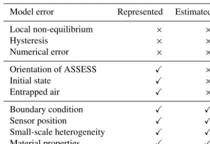
[image:6.612.109.487.112.234.2]Table 3.This overview includes specification whether the consid-ered model error is represented and explicitly estimated within the scope of this study.
Model error Represented Estimated
Local non-equilibrium × ×
Hysteresis × ×
Numerical error × ×
Orientation of ASSESS X ×
Initial state X ×
Entrapped air X ×
Boundary condition X X
Sensor position X X
Small-scale heterogeneity X X
Material properties X X
increased by a larger factor (3.0) if the update is not success-ful.
The described gradient-based algorithm heuristically bal-ances performance and stability. Expanding the stability measures, we introduce a damping vector d with entries
∈(0,1] to decrease the correction of particular parameters via
pi+1=pi+dδpi, (12)
wheredenotes the element-wise Hadamard product. Gen-erally, the entries of the damping vector are set to 1. In order to delay the improvement for parameters which represent ad-ditional model components, we choose the according entries to be less than 1. We use this approach in particular to esti-mate sensor positions and Miller scaling factors along with effective soil hydraulic properties (Sect. A1.4). First, these parameters are initialized to neutral values: the modeled sen-sor positions are initialized to the measured sensen-sor positions and the Miller scaling factors to 1.0. Subsequently, the damp-ing vector for the associated parameters is set to 0.1, reduc-ing the applied correction of these parameters to 10 % of the proposed correction by the Levenberg–Marquardt algorithm. Hence, the main focus of the algorithm is to estimate con-sistent effective soil hydraulic properties, whereas the sensor positions and Miller scaling factors are adjusted more gradu-ally.
2.3.2 Assessment of representation errors
By applying theχ2cost function (Eq. 7), it is implicitly as-sumed that the model is perfect aside from white Gaussian noise. This corresponds to complete quantitative understand-ing of reality and a Gaussian error model for the measure-ment data. Structural model–data mismatch indicates that this assumption is invalid. In our case, a Bayesian analysis of the total uncertainty space is not feasible, primarily due to a lack of models, e.g., for hysteresis. Hence, we have to
ne-glect such representation errors and trust that the structural model–data mismatch will reveal any inadequacy. Table 3 gives an overview over the treatment of the representation errors considered in this work. The contribution of repre-sentation errors, which could not be quantified or excluded from the measurement data a priori, is parameterized and ex-plicitly estimated. The remaining structural model–data mis-match or deviation from the prior for the parameters hints at representation errors which should be corrected in the subse-quent iteration of the analysis.
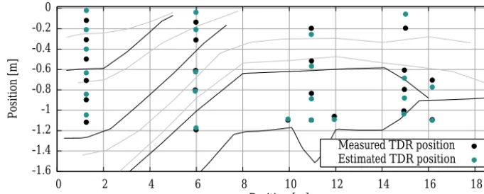
The structural error analysis and the assessment of un-certainties result from iterative evaluations. To illustrate the method, we present an iteration where the orientation of AS-SESS was not yet compensated by rotating the geometry and the gravitation vector (Sect. A1.2). Considering the struc-tural error analysis, we parameterized and estimated uncer-tain components in the representation. Hence, not only the Mualem–Brooks–Corey parameters, an offset to the Dirichlet boundary condition (Sect. A1.5) and the saturated hydraulic conductivity of the gravel layer, but also the position of the TDR sensors were estimated (Sect. A1.4). The results pre-sented in Fig. 5 show that the estimated TDR positions dis-play a consistent deviation from the positions, which were measured relative to the site’s walls, as they compensate for the orientation of ASSESS. Thus, the position of most TDR sensors on the right is estimated to be higher and the position of most TDR sensors on the left is estimated to be lower than that of the measured ones. By estimating the TDR sensor po-sition, we also incorporated other representation errors into the resulting parameters, such as small-scale heterogeneities and eventually a non-represented evaporation front mostly affecting the estimated position of the upper TDR sensors (3, 11, 18, and 25). Hence, this analysis (i) demonstrates the difficulty to separate representation errors and (ii) is able to identify representation errors which have to be improved sub-sequently.
2.3.3 Residual analysis
-1.6 -1.4 -1.2 -1 -0.8 -0.6 -0.4 -0.2 0
0 2 4 6 8 10 12 14 16 18
Position [m]
Position [m]
[image:8.612.127.468.68.205.2]Measured TDR position Estimated TDR position
Figure 5.The subsurface architecture of ASSESS (Fig. 2) is shown with a comparison of measured and estimated TDR sensor positions based on a first evaluation of the hydraulic measurement data. The consistent deviation of the estimated TDR sensor positions reveals an unrepresented model error: the orientation of ASSESS (Sect. A1.2).
measurements. The slope of greater than 1 for large residu-als shows that these residuresidu-als are larger than expected for the presumed Gaussian distribution. Since in this work the the-oretical quantiles are based on a Gaussian distribution, the S shape generally indicates non-Gaussian distributions.
In addition to the visual analysis of the standardized resid-ual, statistical measures help to quantify the model–data mis-match. As a single measure might be misleading (Legates and McCabe, 1999), we calculate the root mean square error (eRMS) and the mean absolute error (eMA).
2.4 Setup
The setup of the parameter estimation is explained in Fig. 6. For each of the three materials, we estimate the Mualem– Brooks–Corey parametersh0,λ,Ks,τ, andθr(Sect. 2.2.2). The saturated water content θs is assumed to be equal to an estimate for the porosity φ based on core samples (Sect. 2.2.4). In order to avoid parameter bias due to rep-resentation errors, we (i) neglect measurement values with volumetric air content smaller 0.1 (Sect. 2.2.4), (ii) esti-mate a constant offset to the Dirichlet boundary condition (Sect. A1.5) and the saturated hydraulic conductivity of the gravel layer, and (iii) developed a method to estimate the ini-tial water content distribution based on TDR measurement data (Sect. A1.6), because a spin-up phase would increase the computation time by up to a factor of 17. The details concerning the implementation of the TDR sensors and the small-scale heterogeneity with Miller scaling factors at the position of the TDR sensors are explained in Sect. A1.4.
In order to analyze the effect of the uncertainty of the sen-sor position, small-scale heterogeneity, and lateral flow on the estimated material properties along the lines presented in Sect. 2.3, we implemented a 1-D and a 2-D study with four different setups.
i. In the basic setup, we estimated the hydraulic material properties, an offset to the Dirichlet boundary condition,
and the saturated hydraulic conductivity of the gravel layer.
ii. With the position setup, we estimated the sensor posi-tions in addition to the parameters in the basic setup. iii. For the Miller setup, we estimated one Miller scaling
factor for each TDR sensor in addition to the parameters in the basic setup.
iv. Finally, in the Miller and position setup, we estimated both the sensor positions and one Miller scaling factor for each TDR sensor in addition to the parameters in the basic setup.
2.4.1 1-D study
In order to investigate the extent to which the experiment at ASSESS can be described with a 1-D model, we set up three different cases with an increasing number of TDR sensors per material (Table 4): case I includes the measurement data of sensor 1 in material C and sensor 2 in material A, and thus comprises one sensor per material. Case II includes two sensors per material: sensors 10 and 11 in material C and sen-sors 12 and 13 in material B. Case III includes three sensen-sors per material: sensors 25, 26, 27 in material A and sensors 28, 29, 30 in material B. Note (i) that the cases are located at dif-ferent positions in ASSESS (Fig. 2) and (ii) that since the hy-draulic potential is not measured in the domain covered with these 1-D studies, the respective inversions are only based on the TDR water content measurements.
ac-Measurement data
Models
Estimation
[image:9.612.49.283.67.256.2]–
Figure 6.The available hydraulic potentialhwtis measured at the bottom of the groundwater wellxλand at the position of the ten-siometerxτ. The data set, which is measured in the groundwater well, is split according to the measurement times: the data measured during the equilibration phasest enter the Levenberg–Marquardt algorithm (Sect. 2.3.1) directly, whereas the data measured during the forcing phases tϕ are only used as a boundary condition for the Richards equation (Sect. 2.2.1). The bulk relative permittivity εb(xµ, tν)and the bulk soil temperatureTb(xµ, tν)are measured at the position of the TDR sensorsxµat timestν. Additionally us-ing the porosityφ (xµ), the bulk permittivity is transferred to wa-ter content (Sect. 2.2.4). The wawa-ter content data enwa-ter the initial state estimation (Sect. A1.6) yielding an initial water content dis-tribution and optional initial parameter values for the Levenberg– Marquardt algorithm. The water content data are also directly used in the Levenberg–Marquardt algorithm. Dashed grey arrows sent one-time preparation steps, whereas solid orange arrows repre-sent the iterative steps of the Levenberg–Marquardt algorithm yield-ing the final material parameterspfinal.
cordingly. Further details concerning the implementation of the 1-D study are given in Sect. A2.1.
For each of the different setups, we ran an ensemble of 20 inversions, starting from Latin hypercube sampled initial parameter sets in order to analyze the convergence behav-ior. The sampling algorithm was implemented with the help of the pyDOE package (https://github.com/tisimst/pyDOE). For each setup, we only analyze the ensemble member with minimalχ2in the subsequent discussion (Sect. 3.1). 2.4.2 2-D study
In this study, we expand the investigated domain to two di-mensions and analyze the performance of the improved rep-resentation. To this end, we set up four different setups (ba-sic, position, Miller, and Miller and position) as described above. Since the positions of both the tensiometer and the groundwater well are in the modeled domain, we use the hydraulic potential measurement data as well as the TDR
Table 4.The 1-D study comprises three different cases which inves-tigate the three materials with an increasing number of TDR sensors per material at different locations in ASSESS (Fig. 2). Note that each material is covered twice.
Case Sensors Materials Position (m)
I 1 and 2 C, A 16.16
II 10, 11 and 12, 13 C, B 10.95
III 25, 25, 27 and 28, 29, 30 A, B 1.26
measurement data in this study. Thus, the position setup is adjusted such that both the positions of TDR sensors and the tensiometer are estimated. All inversions for the 2-D study are initialized with the initial state material functions (Sect. A1.6) in order to bring out the quantitative effect of the different representations on the resulting material prop-erties. Further details concerning the implementation of the 2-D study are given in Sect. A2.2.
3 Results and discussion
In order to improve the quantitative understanding of the hy-draulic behavior of ASSESS (Sect. 2.1), we evaluate a ba-sic representation (Sect. 2.2) with a structural error analysis (Sect. 2.3) that is implemented as outlined in Sect. 2.4. The discussion of the results is done separately for the 1-D study (Sect. 3.1) and the 2-D study (Sect. 3.2).
3.1 1-D study
3.1.1 Objectivity of the measurement data
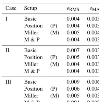
[image:9.612.311.545.117.173.2]Table 5.In order to analyze the results of the 1-D study, the per-formance of the best ensemble members for each case and for each setup are benchmarked with statistical measures. With increasing numbers of included TDR sensors per material, the statistical mea-sures for the basic setup indicate a worse description of the measure-ment data. However, estimating the position and the Miller scaling factor for each TDR sensor improves the description of the mea-surement data significantly according to the statistical measures.
Case Setup eRMS eMA
I Basic 0.004 0.003
Position (P) 0.004 0.003 Miller (M) 0.005 0.004 M & P 0.004 0.003
II Basic 0.007 0.003
Position (P) 0.005 0.003 Miller (M) 0.004 0.003 M & P 0.004 0.003
III Basic 0.009 0.006
Position (P) 0.006 0.004 Miller (M) 0.005 0.003 M & P 0.004 0.002
The large residuals are not random and preferably occur in transient phases. We attribute them to missing processes in the dynamics or to biased parameters. As the curves in the probability plot are basically centered at the origin, a sig-nificant constant bias in the residuum can be excluded. The according statistical measures are given in Table 5.
The eMA of the basic setup increases in case II, because there are two sensors per material and the effective ma-terial parameterization can not completely compensate for the small-scale heterogeneity at the position of both sen-sors simultaneously. Consequently, representing the small-scale heterogeneity improves the description of the data. As before, the largest residuals occur during highly transient phases, especially during the drainage phase. Except for two outliers, the residuals stay smaller than 5 standard deviations here as well. Considering three sensors per material in case III, theeMAincreases even further in the basic setup. Conse-quently, representing small-scale heterogeneities and uncer-tainties in the sensor position in the Miller and position setup improves theeMAby more than a factor of 2.
3.1.2 Separation of uncertain model components Comparing the resulting material properties of the evaluated ensemble members for the different cases and setups (Fig. 8), we notice that the resulting soil water characteristic functions are shifted within each material. During static phases, and if only few measurement sensors are available, the parame-ters for the estimated uncertain model components (Sect. 2.4) can be correlated. However, during transient phases and if a larger number of measurement sensors are available, the
distinct properties of these uncertain model components are more clearly pronounced (Fig. 9 and Sect. 3.2.3).
We also ran the inversions without estimating the offset to the Dirichlet boundary condition (Sect. A1.5), which are not shown here. Besides destabilizing the convergence of the Levenberg–Marquardt algorithm, this fully transfers the un-certainty in the boundary condition to the sensor position. Hence, setups that estimate the sensor position clearly out-perform the others. Additionally, this does not remove the shift of the soil water characteristics.
3.1.3 Lateral flow
The three cases cover the three materials at different loca-tions in ASSESS and are based on distinct data with respect to both quantity and data range.
This is most evident for material A which is located at the bottom of ASSESS and nearly saturated in case I, whereas it is at the top and rather dry in case III (colored dots in Fig. 2). To illustrate that this leads to a different sensitivity on the un-represented model errors, we highlight one example which is most pronounced during the final equilibration phase. In case III, the water content at the position of TDR sensors 25, 26, and 27 is higher than that in static hydraulic equilibrium, leading to a drainage flux and a decrease in water content (Fig. 4). However, in case I, at the position of TDR sensor 2, the water content increases as the sensor monitors the relax-ation of the capillary fringe. Due to the different hydraulic properties of the materials in ASSESS, this relaxation also includes unrepresented lateral flow.
In order to minimize the structural model–data mismatch during this equilibration phase, the parameter estimation al-gorithm increases the hydraulic conductivity to compensate for the non-represented lateral flow with additional vertical flow from above the sensor. Hence, the hydraulic conductiv-ity of case I is larger than the hydraulic conductivconductiv-ity for both case III and the 2-D study, which is discussed in Sect. 3.2.4.
The measurement data of material B used in the inversions of case II and case III do not emphasize the relaxation of the capillary fringe strongly. Hence, we expect that the ef-fect of the unrepresented lateral flow is not as significant as for material A, leading to relatively congruent resulting ma-terial functions. This expectation is confirmed by the results, except for those setups of case II, in which no Miller scaling factor was estimated. These setups show a larger curvature of the soil water characteristic and of the hydraulic conductiv-ity function which is explained in Sect. 3.2.4 in more detail. Additionally, we can identify the previously discussed shift of the soil water characteristic (Sect. 3.1.2).
-10 -5 0 5 10
0 5 10 15 20 25 30 35 40
(a) (b)
(c) (d)
(e) (f)
Standardized residual
Case I
-10 -5 0 5 10
-10 -5 0 5 10
(a) (b)
(c) (d)
(e) (f)
Case I
-10 -5 0 5 10
0 5 10 15 20 25 30 35 40
(a) (b)
(c) (d)
(e) (f)
Standardized residual
Case II
-10 -5 0 5 10
-10 -5 0 5 10
(a) (b)
(c) (d)
(e) (f)
Case II
-10 -5 0 5 10
0 5 10 15 20 25 30 35 40
(a) (b)
(c) (d)
(e) (f)
Standardized residual
Time [h] Case III
-10 -5 0 5 10
-10 -5 0 5 10
(a) (b)
(c) (d)
(e) (f)
Theoretical quantiles Case III
(a) (b)
(c) (d)
(e) (f)
[image:11.612.143.452.64.373.2]Basic Position (P) Miller (M) M & P
Figure 7.For the 1-D study, the standardized residuals of the best ensemble member are visualized over time(a, c, e)and over the theoretical quantiles of a Gaussian with the estimated standard deviation of the TDR measurements (0.007;b,d,f). The cases are analyzed with four setups: basic, position, Miller, and Miller and position. The more sensors per material are used in the inversion, the worse the representation of the basic setup gets. In this case, representing uncertainties with respect to the sensor position and small-scale heterogeneities improves the representation substantially. The decreasing slope of a linear fit (thin lines in the probability plots), which is based on the standardized residuals within[−2,2]theoretical quantiles, also indicates this improvement.
3.1.4 Quality of the initial state material functions The curvature of the soil water characteristic for the inver-sion results is reasonably close the initial state material func-tions (Sect. A1.6), although the initial parameter sets for the 1-D inversions were obtained with Latin hypercube sam-pling. This allows to use the initial state material functions to initialize gradient-based inversion methods. The estimate of the initial state material function for material C deviates strongest from the inversion results compared to the other two materials, since in material C only few sensors are avail-able to assess the form of the capillary fringe. Naturally, the better the available number of TDR sensors is spread over the water content range, the better the fit of the initial state parameters gets. Iteratively restarting the inversion using the previous inversion results as initial state material functions is likely to improve the representation. SinceKsandτ are not estimated along with the initial water content distribution but prescribed a priori, the hydraulic conductivity functions as-sociated with the initial state show large deviations from the inversion results.
3.2 2-D study
3.2.1 Objectivity of the measurement data
-1.4 -1.2 -1 -0.8 -0.6 -0.4 -0.2 0
0 0.1 0.2 0.3 0.4
(a) (b)
(c) (d)
(e) (f)
hm
[m]
Material A
-10 -9 -8 -7 -6 -5 -4 -3
0 0.1 0.2 0.3 0.4
(a) (b)
(c) (d)
(e) (f)
K [m s
-1 ] (log10)
Material A
-1.4 -1.2 -1 -0.8 -0.6 -0.4 -0.2 0
0 0.1 0.2 0.3 0.4
(a) (b)
(c) (d)
(e) (f)
hm
[m]
Material B
-10 -9 -8 -7 -6 -5 -4 -3
0 0.1 0.2 0.3 0.4
(a) (b)
(c) (d)
(e) (f)
K [m s
-1 ] (log10)
Material B
-1.4 -1.2 -1 -0.8 -0.6 -0.4 -0.2 0
0 0.1 0.2 0.3 0.4
(a) (b)
(c) (d)
(e) (f)
hm
[m]
Water content [-] Material C
-10 -9 -8 -7 -6 -5 -4 -3
0 0.1 0.2 0.3 0.4
(a) (b)
(c) (d)
(e) (f)
K [m s
-1 ] (log10)
Water content [-] Material C
(a) (b)
(c) (d)
(e) (f)
[image:12.612.127.468.67.400.2]Case I Case II Case III Initial state
Figure 8.The estimated material functions of the best ensemble member are shown for each of the three cases (case I, case II, and case III) and the four setups of the 1-D study. Additionally, we present the material functions resulting from the initial state estimation (Sect. A1.6). The plot range is adjusted to the available water content range for all inversion results. The number of water content measurements within intervals of 0.05 is indicated with histogram bars for each case. The height of these bars is normalized over all figures in this work. The main message of this figure is that unrepresented model errors may lead to biased hydraulic parameters. In particular, this can be seen by comparing the hydraulic conductivityKof material A for cases I and III.
in the basic setup increase, and (iii) estimating sensor posi-tions and Miller scaling factors improves the description of the TDR data significantly. The standardized residuals con-firm the last two expectations (Fig. 10). However, similar to the 1-D study, even the residuals of the Miller and position setup still reach more than 5 standard deviations for the 2-D representation.
In order to understand this deviation in more detail, we in-vestigate the remaining structural model–data mismatch dur-ing the final drainage and equilibration phases between 30 and 40 h. The largest residuals occurring during the drainage phase around 30 h come from TDR sensors 6, 9, 13, and 17. We identified that these sensors are located close to a com-paction interface (Sect. A1.6). Hence, the large residuals in-dicate that this horizontal compaction layer is not correctly represented with a point-scale representation of the small-scale heterogeneity.
The largest residuals during the final equilibration phase between 30–40 h come from TDR sensors 2 and 22 close to the capillary fringe. We attribute them to unrepresented processes in the dynamics, such as hysteresis or 3-D flow (Sect. 3.2.2).
-1
-0.8
-0.6
-0.4
-0.2
0
0.2
0.05 0.1 0.15 0.2 0.25 0.3 0.35 0.4
(z - z
0
) [m]
Water content [-]
[image:13.612.62.275.67.197.2]Material properties (h0, λ) TDR sensor position Small-scale heterogeneity Groundwater table
Figure 9.The estimation of uncertain model components can lead to correlated estimated parameters, e.g., as an incorrect position of the groundwater table (z0) can be compensated by changingh0and λduring static phases. During transient phases, however, the com-ponents have distinct effects, e.g., asλalso changes the conductivity function. Hence, the ability of the parameter estimation algorithm to separate these uncertainties depends on the available measure-ment data. Also, the more sensors are available, the fewer uncertain model components can be compensated simultaneously by the pa-rameterization.
0.001, 0.007, and 0.006 m for the water content, tensiome-ter, and manual groundwater position data, respectively. With complete quantitative understanding (Sect. 2.3), the standard deviation of the residuals would correspond to this precision. Lacking ground truth, the accuracy of the measurement data is unknown a priori and may depend on the hydraulic state. In this study, its estimated contribution dominates the size of the standard deviations. Our results show that the model can represent static phases better than highly transient phases and that the accuracy of the measurement data is higher than that estimated a priori. The statistical measures for the water con-tent data given in Table 6 reveal that the eMA of the basic setup merely increases by less than a factor of 2 compared to case III of the 1-D study. Estimating sensor positions and Miller scaling factors improves the description of the TDR measurement data by more than a factor of 2 leading to a
eMAof 0.004.
3.2.2 Hydraulic potential
The description of the hydraulic potential data only improves in those setups in which the sensor position is estimated (Fig. 10 and Table 6). Also, the temporal structure of the model–mismatch does not change significantly with the dif-ferent setups. The data show a gradient of the hydraulic pres-sure between the tensiometer and the groundwater well dur-ing the forcdur-ing phases (Fig. 3). Considerdur-ing symmetry, we also assume this gradient of the hydraulic potential in the ne-glected third dimension. Hence, the forcing via the ground-water well leads to a 3-D ground-water flux during the experiment. This makes a correct representation of the groundwater ta-ble impossita-ble in 2-D. Consequently, the simulation should
Table 6.For each setup of the 2-D study, the results are bench-marked with statistical measures. Similar to the 1-D study, estimat-ing the sensor position and the Miller scalestimat-ing factors improves the statistical measures related to the water content significantly. The statistical measures for the position of the groundwater table in-cluding both the tensiometer and the groundwater well data improve only for setups in which the sensor positions are estimated.
Water content Water table
Setup eRMS eMA eRMS eMA
Basic 0.017 0.011 0.04 0.03 Position (P) 0.011 0.006 0.02 0.02 Miller (M) 0.008 0.005 0.03 0.03 M & P 0.006 0.004 0.02 0.02
predict a higher position of the groundwater table in the well during imbibition phases and a lower groundwater table dur-ing the drainage phases. This expectation is confirmed by the standardized residuals shown in Fig. 10. Thus, the struc-tural model–data mismatch of the tensiometer data indicates that employing the groundwater table as a Dirichlet bound-ary condition overestimates the forcing in the simulation. Therefore, the simulated hydraulic pressure during the imbi-bition is larger than the measured one which leads to neg-ative residuals. As expected, this behavior reverses during drainage phases.
3.2.3 Separation of uncertain model components The 2-D study is based on a larger number of water con-tent measurements, additional hydraulic pocon-tential measure-ments, and more complicated flow phenomena compared to the previously discussed 1-D study (Sect. 3.1). This improves the ability of the Levenberg–Marquardt algorithm to separate uncertain model components (Sect. 3.1.2) and decreases the shift in the soil water characteristics of the different setups compared to the 1-D study (Fig. 11).
3.2.4 Effect of unrepresented model errors
Each setup starts from the same initial material functions (Sect. A1.6). Therefore, the difference between the resulting material properties of the setups (Fig. 11) is a direct conse-quence of the representation of uncertainties in the sensor position and small-scale heterogeneities.
[image:13.612.332.523.152.235.2]-15 -10 -5 0 5 10 15
0 5 10 15 20 25 30 35 40
(a) (b)
(c) (d)
(e) (f)
Standardized residual
TDR
-15 -10 -5 0 5 10 15
-15 -10 -5 0 5 10 15
(a) (b)
(c) (d)
(e) (f)
TDR
-4 -2 0 2 4
0 5 10 15 20 25 30 35 40
(a) (b)
(c) (d)
(e) (f)
Standardized residual
Groundwater well
-4 -2 0 2 4
-4 -2 0 2 4
(a) (b)
(c) (d)
(e) (f)
Groundwater well
-4 -2 0 2 4
0 5 10 15 20 25 30 35 40
(a) (b)
(c) (d)
(e) (f)
Standardized residual
Time [h] Tensiometer
-4 -2 0 2 4
-4 -2 0 2 4
(a) (b)
(c) (d)
(e) (f)
Theoretical quantiles Tensiometer
(a) (b)
(c) (d)
(e) (f)
[image:14.612.136.458.64.386.2]Basic Position (P) Miller (M) M & P
Figure 10.The standardized residuals of the 2-D study are visualized over time(a, c, e)and in a probability plot(b, d, f)for all TDR and hydraulic potential sensors. The color associates the results with the four setups of the study (basic, position, Miller, and Miller and position). Same as for the 1-D study, the standard deviation for the TDR measurement data is chosen as 0.007. We choose the standard deviation for both the manual measurements in the groundwater well and the tensiometer measurement data as 0.025 m. The representation of uncertainties with respect to the sensor positions and small-scale heterogeneities improves the description of the TDR data quantitatively. The decreasing slope of a linear fit (thin lines in the probability plots), which is based on the standardized residuals within[−2,2]theoretical quantiles, also indicates this improvement. The structural model–data mismatch for the hydraulic potential data is mainly due to (i) uncertainties concerning the position of the tensiometer and (ii) unrepresented 3-D flow phenomena.
Table 7.We present the effective hydraulic material parameters obtained with the Miller and position setup of the 2-D study. The formal standard deviations of the parameter estimation are given with the understanding that these are specific to the applied algorithm and will change for different algorithm parameters. The estimations for the saturated hydraulic conductivity of the gravel layer and for the offset to the Dirichlet boundary condition are 10−0.728±0.006m s−1and−0.034±0.001 m, respectively.
Material h0(m) λ (−) Ks(m s−1) τ (−) θr(−) θs(−) A −0.184±0.005 1.94±0.07 10−4.212±0.004 0.33±0.07 0.025±0.004 0.41 B −0.174±0.004 2.54±0.06 10−3.77±0.02 0.78±0.05 0.035±0.001 0.36 C −0.159±0.004 3.28±0.02 10−3.70±0.02 0.74±0.06 0.026±0.002 0.38
0.8 and 1.4 m above the groundwater table (sensors 28 and 18). If the uncertainty in sensor position and small-scale het-erogeneities are represented in the model, the outlying mea-surement data can be described without altering the effective material properties.
It is worth noting that although the uncertainty of the mea-sured grain size distribution (Table 1) is large, the resulting
[image:14.612.101.495.554.612.2]-1.4 -1.2 -1 -0.8 -0.6 -0.4 -0.2 0
0 0.1 0.2 0.3 0.4
(a) (b)
(c) (d)
(e) (f)
hm
[m]
Material A
-10 -9 -8 -7 -6 -5 -4 -3
0 0.1 0.2 0.3 0.4
(a) (b)
(c) (d)
(e) (f)
K [m s
-1 ] (log10)
Material A
-1.4 -1.2 -1 -0.8 -0.6 -0.4 -0.2 0
0 0.1 0.2 0.3 0.4
(a) (b)
(c) (d)
(e) (f)
hm
[m]
Material B
-10 -9 -8 -7 -6 -5 -4 -3
0 0.1 0.2 0.3 0.4
(a) (b)
(c) (d)
(e) (f)
K [m s
-1 ] (log10)
Material B
-1.4 -1.2 -1 -0.8 -0.6 -0.4 -0.2 0
0 0.1 0.2 0.3 0.4
(a) (b)
(c) (d)
(e) (f)
hm
[m]
Water content [-] Material C
-10 -9 -8 -7 -6 -5 -4 -3
0 0.1 0.2 0.3 0.4
(a) (b)
(c) (d)
(e) (f)
K [m s
-1 ] (log10)
Water content [-] Material C
(a) (b)
(c) (d)
(e) (f)
Basic Position (P)
Miller (M) M & P
[image:15.612.133.463.65.398.2]Initial state 1-D study
Figure 11.We show the resulting material functions for all three materials involved in the 2-D study which is analyzed with the four setups (basic, position, Miller, and Miller and position). The plot range is adjusted to the available water content range for each material. The height of the histogram bars denotes the number of available water content measurements and is normalized over all figures in this work. Since the inversions for all setups are initialized with the material functions resulting from the initial state estimation (Sect. A1.6), the difference between the results is directly linked to the estimation of sensor positions and small-scale heterogeneities. For direct comparison, the results of the 1-D study are also shown.
4 Summary and conclusions
We applied a structural error analysis on a representation of the effectively 2-D architecture ASSESS. This representa-tion includes TDR and hydraulic potential measurement data which were acquired during a fluctuating groundwater table experiment. Based on the assumption that structural model– data mismatch indicates incomplete quantitative understand-ing of reality, we implemented a 1-D and a 2-D study orga-nized in different setups with increasingly complex models. We started with the estimation of effective hydraulic material properties and we added the estimation of sensor positions, small-scale heterogeneity, or both. It was demonstrated that the structural error analysis can indicate significant unrepre-sented model errors, such as the slope of the ASSESS test site.
We showed that estimated material properties resulting from a 1-D study are biased due to unrepresented lateral flow. Analyzing representations with increasing data quantity, it
was also found that the fewer sensors are available per mate-rial, the stronger is the influence of the unrepresented model errors on the estimated material properties. We illustrated that the more complicated flow phenomena are represented, the better uncertain model components can be separated by the parameter estimation algorithm leading to more reliable material properties. Generally, representing sensor position uncertainty and small-scale heterogeneity improved the de-scription of the water content data quantitatively in setups with many sensors. Yet, the residuals of the water content data still reach more than 5 standard deviations during tran-sient phases (Fig. 10). We attribute this to remaining repre-sentation errors in the dynamics, forcing, and compaction in-terfaces.
of the soil water characteristic. We found that this approxi-mation is reasonably close to inversion results and that the according parameters can be used as initial parameters for gradient-based optimization. Since all the inversions of the 2-D study are initialized with these parameters, the compar-ison of the results directly displays the quantitative effect of the according unrepresented model errors on the estimated material properties.
Since the three approaches ((i) initial state estimation, (ii) 1-D inversion, and (iii) 2-D inversion) allow to estimate effective hydraulic material parameters, we finally discuss their levels of improving the quantitative understanding of soil water dynamics.
The initial state estimation requires at least three water content measurements per material over the full water con-tent range and the position of the groundwater table to es-timate the parameters for soil water characteristic for one specific equilibrated hydraulic state. Lacking direct measure-ments of the unsaturated hydraulic conductivity, the method cannot estimate the remaining parametersKsandτ required to model soil water dynamics. Additionally, it is highly sus-ceptible to uncertainties related to the sensor position and small-scale heterogeneities. Yet, the method is fast (a few seconds on a local machine) and suitable for providing initial parameters for gradient-based inversion methods.
The 1-D inversions are comparably fast (several minutes up to several hours on a local machine) and can represent transient states. In contrast to the initial state estimation, 1-D inversions can estimate all parameters of the material func-tions. However, more complicated flow phenomena includ-ing lateral flow can not be represented. This leads to biased parameters.
The unique characteristics of the 2-D inversions (days on a cluster with same number of cores as parameters) is the abil-ity to represent lateral flow phenomena which are typically monitored with a high number of sensors. Hence, the consis-tency of the representation is implicitly checked. Therefore, we expect that of the three approaches discussed, this one yields the most reliable material properties. Still, unrepre-sented model errors including 3-D flow phenomena influence the results.
Appendix A: Details of the implementation A1 Representation
A1.1 Richards equation solver
The Richards equation (Eq. 1) is solved numerically with
µϕ(muPhi, Ippisch et al., 2006) on a rectangular structured grid using a cell-centered finite volume scheme with full up-winding in space and an implicit Euler scheme in time. The non-linear equations are linearized with an inexact Newton method with line search and the linear equations are solved with an algebraic multigrid solver.
A1.2 Orientation of ASSESS
ASSESS is not built completely rectangular. Most impor-tantly, both the surface and the ground are not horizontal but primarily inclined towards the groundwater well with a mean slope of≈ −0.1
20 = −0.005. Since the applied Richards solver µϕdemands a rectangular structured grid, the geometry was rotated. This rotation was compensated by a counter-rotation of the gravity vectorg≈(0.0708,−9.8097)>.
A1.3 Evaluation of TDR traces
The volumetric water content is evaluated from measured TDR traces (Fig. A1). As inflection points of the measured signal can be chosen to mark the reflections at the probe head and at the end of rods, the evaluation of the two-way signal travel time is based on detecting the maxima of the first tem-poral derivative of the recorded trace. To increase the pre-cision of the evaluation, parabolas are fitted to the detected maxima. Finally, the maxima of the parabolas are employed to evaluate the two-way signal travel time. With the help of individual calibration data for each sensor comprising mea-surements in air and desalinated water, the travel time is con-verted into the relative permittivityεbof the bulk.
A1.4 Sensor position and small-scale heterogeneity The numerical solution of the Richards equation (Eq. 1) is discretized in space with a rectangular structured grid (Sect. A1.1). Generally, the simulated value for the modeled position of a sensor is bilinearly interpolated from the simu-lated values at the center of the surrounding grid cells. Due to measurement uncertainties and subsidence after the con-struction, Antz (2010) and Buchner et al. (2012) assess the uncertainty concerning positions of sensors and material in-terfaces in ASSESS to ±0.05 m with respect to the model. However, since imbibition fronts can be very steep in sandy soils (Dagenbach et al., 2013; Klenk et al., 2015) and the measurement volume of the applied sensors is small, fluctu-ating groundwater table experiments are very sensitive to the sensor position. Hence, we (i) enable the parameter estima-tion algorithm (Sect. 2.3.1) to estimate the sensor posiestima-tions
and (ii) implement the measurement volume of the TDR sen-sors by averaging the simulation data within a measurement radius of 0.015 m.
In order to represent the heterogeneity of ASSESS which is not covered by describing the different sand types with dis-tinct material properties due to the small-scale variability of the pore space, the center of each grid cell is associated with a Miller scaling factor (Eq. 4) that is initialized to 1.0. As the information about this small-scale heterogeneity only enters via the TDR measurement data, the exact position of each TDR sensor in the grid is also associated with a Miller scal-ing factor. This scalscal-ing factor may be estimated with the pa-rameter estimation algorithm (Sect. 2.3.1). The scaling fac-tors in the neighborhood of the TDR sensor are determined with a bivariate Gaussian distribution in horizontal and ver-tical directions. This distribution is centered at the position of the TDR sensor and its amplitude corresponds to the as-sociated Miller scaling factor. With a standard deviation of 0.015 m in both directions, it approaches 1.0 with increas-ing distance from the TDR sensor. Finally, this distribution is projected on each grid cell, yielding the applied scaling fac-tors which are only different from 1.0 in the neighborhood of the TDR sensors.
A1.5 Boundary condition
Generally, the boundary of the simulation is implemented with a Neumann no-flow condition. However, during the forcing phases, we prescribe the measured groundwater ta-ble as a Dirichlet boundary condition at the position of the groundwater well. In addition to the orientation of AS-SESS (Sect. A1.2), the uncertainty of the sensor positions (Sect. A1.4) directly translates to an uncertainty in the Dirichlet boundary condition. Since representation errors of the forcing have a large impact on the resulting parameters, we implemented an optional offset to the Dirichlet boundary condition which can be estimated (Sect. 2.4).
A1.6 Initial state estimation
Since we use an inversion method for parameter estimation (Sect. 2.4), starting as close as possible to the measured ini-tial state is key. Usually, this is achieved with a spin-up phase; however, it is computationally very expensive.
Hence, we developed a method to estimate the initial water content distribution based on TDR measurement data.
mea--0.6 -0.4 -0.2 0 0.2 0.4 0.6
0 1 2 3 4 5 6 7 8 9 -0.6 -0.4 -0.2 0 0.2 0.4 0.6
Reflection coefficient [-]
Reflection coefficient per time [ns
-1 ]
[image:18.612.128.466.69.206.2]Travel time [ns] Measured trace Temporal derivative Parabola fits Signal travel times
Figure A1.The evaluation of a TDR trace is based on the detection of the inflection points caused by the probe head and the end of the rod. This is done automatically after calculating of the first temporal derivative of the trace. Parabolas are fitted to the maxima of the temporal derivative to increase the precision of the evaluated signal travel time.
sured water content. For each material, we then fit the param-etersh0,λ, andθrof the Brooks–Corey parameterization to the approximated matric potential and the measured water content (Fig. A2). The saturated water contentθsis assumed to be known from core samples. This yields an approxima-tion for the initial water content distribuapproxima-tion between the TDR sensors. With the resulting parameter values for each material, the subsurface material distribution, and the posi-tion of the groundwater table, we can calculate an estimaposi-tion of the initial water content distribution in ASSESS (Fig. A3). As the parameters for the Brooks–Corey parameteriza-tion are derived from static measurement data, we may use them as initial parameter values for computationally expen-sive gradient-based inversions of dynamic measurement data (Sect. 2.4.2). The missing initial parameter values τ =0.5 andKs=8.3·10−5m s−1are taken from Carsel and Parrish (1988). We refer to these parameter sets as initial state mate-rial functions in this work.
In particular due to (i) a limited number of TDR sensors, (ii) missing hydraulic potential measurements at the position of the TDR sensors, and (iii) spatial small-scale heterogene-ity present in the materials, structural deviations between the estimation and the measurements occur, which indicate lim-itations of describing ASSESS with effective soil hydraulic material properties.
The water content measured by TDR sensors 5, 12, and 29 deviate structurally from the estimation of the initial state for material B (Fig. A2). Klenk et al. (2015, Figs. 1b and 6) presented GPR measurements which indicate that at least TDR sensors 6, 9, 13, 17, and 22 are closely below a com-paction interface. However, the position of this interface was not measured during the construction process. Thus, these TDR sensors are monitoring a compacted pore structure. In contrast, TDR sensors 5, 12, and 29 are situated in rather undisturbed areas. Hence, as most of the TDR sensors are influenced by the compaction interfaces, the analysis of this measurement data is likely to underestimate the effective
wa-ter content leading to a biased soil wawa-ter characwa-teristic for material B. This is a typical situation encountered with point-like sensors in heterogeneous media.
A2 Setup A2.1 1-D study
The forward simulations were calculated with a grid reso-lution of 0.005 m and 10−8 as a limit of the Newton solver (Sect. A1.1). Following Jaumann (2012), the standard devi-ation of the TDR measurements is assumed as 0.007. We use the manually measured groundwater table data as a Dirichlet boundary condition. Uncertainties concerning the position of the sensors and the subsurface material inter-faces directly translate to uncertainties in the boundary con-dition (Sect. A1.5). Accounting for the orientation of AS-SESS (Sect. A1.2), we add a constant offset to the Dirichlet boundary condition for each case (case I:−0.02 m, case II:
−0.05 m, case III:−0.12 m). In order to minimize the input error, we also estimate this offset in the inversion. If TDR sensor positions are estimated, these are initialized to the measured position. Similarly, the Miller scaling factors are initialized to 1.0.
A2.2 2-D study
The 2-D simulations in this work are calculated with a grid resolution of 0.2 m×0.02 m. The limit of the Newton solver is set to 10−8 (Sect. A1.1). Like for the 1-D studies, we choose 0.007 as the standard deviation of the TDR measure-ments. The standard deviation of the tensiometer (0.025 m) is assessed from the accuracy (±5 hPa) as specified by the man-ufacturer. In order to transfer the given uniform distribution with range±5 hPa≈ ±0.05 m to a Gaussian distribution, we associate this range with the 2σ interval of a Gaussian (5 to 95 %). This leads to an approximate standard deviation of
0 0.2 0.4 0.6 0.8 1 1.2 1.4
0 0.1 0.2 0.3 0.4
(a) (b) (c)
(z - z
0
) [m]
Water content [-] Material A
0 0.2 0.4 0.6 0.8 1 1.2 1.4
0 0.1 0.2 0.3 0.4
(a) (b) (c)
Water content [-] Material B
0 0.2 0.4 0.6 0.8 1 1.2 1.4
0 0.1 0.2 0.3 0.4
(a) (b) (c)
Water content [-] Material C
(a) (b) (c)
[image:19.612.126.468.68.207.2]Estimation Measurement
Figure A2.We use the Brooks–Corey parameterization to estimate the initial water content distribution between the TDR sensors. As-suming hydraulic equilibrium, we approximate the matric potentialhmwith the negative distance to the groundwater table positionz0: hm≈ −(z−z0). For each material, we then use the approximated matric potential at the position of the TDR sensors and the corresponding water content measurement data to fit the Brooks–Corey parameters. Each dot depicts the mean of 15 subsequent data points measured in the 4 h preceding the experiment. The according standard deviations are all smaller than 0.002, which indicates (i) that the hydraulic system is relatively equilibrated at the beginning of the experiment and (ii) that the deviations from the estimation are statistically significant.
-1.8 -1.6 -1.4 -1.2 -1 -0.8 -0.6 -0.4 -0.2 0
2 4 6 8 10 12 14 16 18
Position [m]
Position [m] -1.8
-1.6 -1.4 -1.2 -1 -0.8 -0.6 -0.4 -0.2 0
2 4 6 8 10 12 14 16 18
0.05 0.1 0.15 0.2 0.25 0.3 0.35 0.4
Water content [-]
1
2 3
4 5 6 7 9
10
11
12
13
14 17 18
19
20 21
22 25
26 27 28 29
30
31 A
B
C
C
B
A
Figure A3.The estimated initial water content distribution is based on the TDR measurement data (Fig. A2, shown as face color of the circled dots). Since the saturated water contentθsis fixed for each material a priori, only TDR sensors in unsaturated material are shown. Due to the orientation of ASSESS (Sect. A1.2), the groundwater table is slightly slanted. The black lines indicate material interfaces, whereas the white lines indicate compaction interfaces, which were introduced during the construction of ASSESS. Note the different scales on the horizontal and vertical axes.
[image:19.612.126.467.298.433.2]