Post processing rainfall forecasts from numerical weather prediction models for short term streamflow forecasting

www.hydrol-earth-syst-sci.net/17/3587/2013/ doi:10.5194/hess-17-3587-2013

© Author(s) 2013. CC Attribution 3.0 License.

Hydrology and

Earth System

Sciences

Post-processing rainfall forecasts from numerical weather

prediction models for short-term streamflow forecasting

D. E. Robertson, D. L. Shrestha, and Q. J. Wang

CSIRO Land and Water, P.O. Box 56, Highett, 3190 Victoria, Australia

Correspondence to: D. E. Robertson ([email protected])

Received: 3 May 2013 – Published in Hydrol. Earth Syst. Sci. Discuss.: 29 May 2013 Revised: 15 August 2013 – Accepted: 15 August 2013 – Published: 27 September 2013

Abstract. Sub-daily ensemble rainfall forecasts that are bias free and reliably quantify forecast uncertainty are critical for flood and short-term ensemble streamflow forecasting. Post-processing of rainfall predictions from numerical weather prediction models is typically required to provide rainfall forecasts with these properties. In this paper, a new approach to generate ensemble rainfall forecasts by post-processing raw numerical weather prediction (NWP) rainfall predictions is introduced. The approach uses a simplified version of the Bayesian joint probability modelling approach to produce forecast probability distributions for individual locations and forecast lead times. Ensemble forecasts with appropriate spa-tial and temporal correlations are then generated by linking samples from the forecast probability distributions using the Schaake shuffle.

The new approach is evaluated by applying it to post-process predictions from the ACCESS-R numerical weather prediction model at rain gauge locations in the Ovens catch-ment in southern Australia. The joint distribution of NWP predicted and observed rainfall is shown to be well described by the assumed log-sinh transformed bivariate normal dis-tribution. Ensemble forecasts produced using the approach are shown to be more skilful than the raw NWP predictions both for individual forecast lead times and for cumulative to-tals throughout all forecast lead times. Skill increases result from the correction of not only the mean bias, but also biases conditional on the magnitude of the NWP rainfall prediction. The post-processed forecast ensembles are demonstrated to successfully discriminate between events and non-events for both small and large rainfall occurrences, and reliably quan-tify the forecast uncertainty.

Future work will assess the efficacy of the post-processing method for a wider range of climatic conditions and also

investigate the benefits of using post-processed rainfall fore-casts for flood and short-term streamflow forecasting.

1 Introduction

Forecasts of streamflow are valuable to a range of users. Forecasts of potential flood conditions provide emergency and water managers with the opportunity to plan mitigation strategies and responses such as evacuations (Roulin, 2007; Penning-Rowsell et al., 2000; Blöschl, 2008). Forecasts of within bank streamflow events, such as freshes and low flow conditions, allow water managers to optimise water distribu-tion, minimise potential damage to private property and max-imise environmental benefits in regulated streams (George et al., 2011). All these water management actions can poten-tially have a range of costs and benefits and therefore fore-cast users require an indication of forefore-cast uncertainty to al-low the risks associated with management decisions to be assessed.

In Australia, numerical weather prediction (NWP) mod-els provide forecasts of weather conditions for lead times of up to 10 days. However, raw output that is publicly avail-able from Australian NWP models is deterministic and often contains systematic errors (Shrestha et al., 2013). These er-rors can emerge from two major sources (Ebert, 2001). Fine-scale physical processes are parameterized in NWP models in order to run them at the relatively coarse spatial and verti-cal resolutions necessary for routine operational applications. NWP models also require the initial conditions of the atmo-sphere and land/sea surface to be specified for each forecast. Both the model parameterizations and initial conditions are potential sources of systematic forecast errors. Outside Aus-tralia, ensemble predictions systems have been developed to reduce systematic errors and quantify forecast uncertainty by producing multiple runs of the NWP model with varying initial conditions or model parameterizations. However the spread of the ensemble is commonly too narrow and there-fore not reliable in a probabilistic sense (Hamill and Colucci, 1997; Santos-Muñoz et al., 2010; Clark et al., 2011).

Statistical calibration or post-processing methods are fre-quently applied to correct biases and produce forecasts that reliably quantify uncertainty. Many methods use some form of probability model to post-process forecasts for a single forecast period and location (Wilks, 2006; Schaake et al., 2007; Wu et al., 2011; Kleiber et al., 2010; Sloughter et al., 2007; Glahn and Lowry, 1972; Hamill et al., 2004). A com-mon approach for meteorological applications is to use a two part probability model, where the probability of precipita-tion occurrence is post-processed using logistic regression and the rainfall amount modelled using a Gamma distribu-tion condidistribu-tioned on the raw NWP output (Sloughter et al., 2007). There are numerous variants of this approach using different transformations for NWP predicted rainfall, and ob-served rainfall and levels of complexity in the logistic regres-sion and Gamma distribution conditioning models (Hamill et al., 2004; Sloughter et al., 2007). Generalising the approach requires a considerable number of parameters and risks over-fitting. For hydrological applications, methods which model the joint distribution of NWP rainfall predictions and their corresponding observations have been developed (for exam-ple, Wu et al., 2011; Schaake et al., 2007). These joint distri-bution modelling methods have complex parameterizations and require the appropriate transformations for data nor-malisation or marginal distributions to be selected at each location.

Post-processed NWP rainfall predictions produced by ap-plying a probability model to each forecast period and lo-cation separately will not contain the appropriate spatial and temporal correlation structures necessary for stream-flow forecasting applications (Clark et al., 2004; Schaake et al., 2007; Wu et al., 2011). Statistical post-processing methods which explicitly model spatial and temporal cor-relations structures are typically computationally expensive and are yet to be widely adopted for operational streamflow

forecasting applications. To overcome these computational challenges, Clark et al. (2004) described the “Schaake shuf-fle” which produces ensemble forecasts by linking samples from discretely post-processed forecasts to follow histori-cally observed spatial and temporal correlation patterns.

Recently, the Bayesian joint probability (BJP) modelling approach (Wang and Robertson, 2011; Wang et al., 2009) has successfully post-processed seasonal rainfall predictions from the global climate model (POAMA) effectively re-moving biases and reliably quantifying forecast uncertainty (Wang et al., 2012a; Charles et al., 2011). The formulation of the BJP modelling approach is similar to the methods de-scribed by Wu et al. (2011) and Schaake et al. (2007), and therefore it may also be useful for post-processing sub-daily rainfall predictions. The advantage of the BJP modelling ap-proach is that it provides a highly flexible probability model with relatively few parameters, through its use of a paramet-ric transformation for data normalisation and variance sta-bilisation, and Bayesian parameter inference methods. How-ever, sub-daily rainfall totals have a more highly skewed dis-tribution and considerably greater intermittency of precipi-tation than seasonal rainfall totals, and therefore the perfor-mance of the approach may be limited due to shortcomings in the parametric transformation and the treatment of precip-itation intermittency as a problem of censored data.

The objective of this study is twofold. Firstly we assess whether the BJP modelling approach can be effectively used to post-process sub-daily rainfall predictions from a deter-ministic NWP model for single forecast lead times. Secondly we assess the performance of ensemble rainfall forecasts pro-duced by linking samples from the post-processed proba-bilistic forecasts using the Schaake shuffle, demonstrating that the post-processed forecasts are more skilful than the raw output from the NWP and that the forecast uncertainty is reliably quantified.

The remainder of the paper is structured as follows. The next section describes the NWP predictions and observed data used in this study. Section 3 describes the implementa-tion of the BJP modelling approach for post-processing sub-daily rainfall predictions and methods used to check model assumptions and verify forecasts. Section 4 presents results for model checking and forecast verification. In Sect. 5, we discuss the potential limitations of the method and the cur-rent application, and identify possible extensions. Section 6 provides a summary of the paper and draws conclusions.

2 Study catchment and data

flooding. The time of concentration to the catchment outlet is of the order of four to five days; however the time of concen-tration to some flood sensitive areas within the catchment can be less than 24 h and therefore hydrological models are run at sub-daily time steps (Pagano et al., 2011).

Hourly observed precipitation data were obtained from the operational flood forecasting database of Australian Bu-reau of Meteorology for 33 rain gauges located in the Ovens catchment (Fig. 1). Carboor Upper is highlighted in Fig. 1 as many of the results presented focus on this site. Mean annual rainfall at the 33 gauges locations varies between 550 mm, near the catchment outlet, and 1950 mm in the catchment headwaters. An historical archive of hourly precipitation data is available from September 1991. However as the data are observations used operationally, the archive contains missing records for some locations and times. Rain gauge data were used for this study rather than the subcatchment rainfall used for real-time forecasting. This was done to limit the influence of artefacts resulting from missing data that are introduced by the interpolation techniques currently in operational use.

Rainfall predictions were obtained from the Australian Community Climate Earth-System Simulator (ACCESS). Several variants of the ACCESS model are used to form the Australian Parallel Suite (APS), which is the basis of nu-merical weather prediction in Australia (Australian Bureau of Meteorology, 2010). For this study we use predictions from the regional ACCESS model (ACCESS-R) which is run every 12 h (00:00 and 12:00 UTC) at a 37.5 km resolu-tion out to a lead time of 72 h. ACCESS-R data are avail-able at 1 h intervals. The domain of the regional ACCESS model extends from 65◦_{S, 65}◦_{E to 17.125}◦_{N, 184.625}◦_E

and boundary conditions are sourced from the global AC-CESS model, which runs at approximately 80 km resolution. Hindcasts for the ACCESS suite of models are not available. An archive of real-time predictions for a 20 month period (approximately 600 forecasts) extending from January 2010 to August 2011 is available. While a longer record is desir-able it is unlikely to be availdesir-able for operational forecasting applications in Australia.

In operational conditions, streamflow forecasts are issued once a day at 23:00 UTC (09:00 LST – local standard time). For this study we use the most recently issued NWP pre-diction (12:00 UTC) that is available when the streamflow forecasts are made. This means that the first eleven hours of NWP rainfall predictions are neglected and post-processing is applied to NWP predictions between 11 and 72 h after the time of forecast issue. Forecasts for these periods are subse-quently referred to as lead times 0 to 60 h, where lead time 0 forecasts are for the hour commencing 23:00 UTC on the day the forecast is issued.

Fig. 1. Ovens catchment and rain gauge locations.

3 Methods

3.1 Post-processing NWP model rainfall predictions

We apply a modified version of the BJP modelling approach to post-process raw NWP rainfall predictions for individual forecast lead times. Full details of the BJP modelling ap-proach are provided in Wang et al. (2009) and Wang and Robertson (2011) here we present a brief overview to high-light the differences between the original implementation and the application used in this study. In contrast to Wang et al. (2009) and Wang and Robertson (2011) our formula-tion is for a bivariate problem where a single predictor and single predictand are used. The model predictor (y1), in this case NWP rainfall predictions for a single lead time, and pre-dictand (y2), in this case observed rainfall, are arranged as a column vector

y =

y1

y2

.

z= 1

β ln(sinh(α+βy)) ,

whereα andβ are parameters of the transformation. The transformed variables (z) are assumed to follow a bivariate normal distribution z= z1 z2

∼N (µ,6)

where µ= µ1 µ2 and 6 =

σ₁2 r σ1σ2

r σ1σ2σ22

.

The set of model parameters (θ) describe the transformation, using two parameters (αandβ), mean (µ) and standard de-viation (σ) for each predictor and predictand, and correlation coefficients (r). All model parameters are reparameterized to ease parameter inference. Reparameterizations of model pa-rameters are described in the Appendix.

The original formulation of the BJP modelling ap-proach for seasonal forecasting infers model parameters and their uncertainties using Markov chain Monte Carlo methods to sample from the posterior parameter distribu-tion p (θ|YOBS), where YOBS=y1_OBS,y2_OBS, . . . , yn_OBS andyt_OBS is the observed predictor and predictand data for eventt,t= 1, 2, . . . ,n. Formulation of the posterior parame-ter distribution is detailed in the Appendix.

For operational short-term forecasting applications con-siderably more data are available to infer model parameters than for seasonal forecasting applications. This will reduce parameter uncertainty, and computational resources required to infer parameter uncertainties using a large data set may not necessarily be available in real-time. Therefore, in this study we obtain a single set of model parameters that gives the maximum a posteriori (MAP) solution.

We obtain the MAP solution for the joint distribution of model parameters using a stepwise approach. We obtain the parameters describing the MAP solution of the log-sinh transformed normal distribution for the marginal distribu-tion of each predictor and predictand separately. We find the MAP solution using the shuffled complex evolution algo-rithm (Duan et al., 1994) to ensure that a global optimum is found. We then use the parameters describing the MAP solution for the marginal distributions of the predictors and predictands in the joint distribution and infer the matrix of transformed correlation coefficients that describe the MAP solution for the joint log-sinh transformed bivariate normal distribution.

To produce a probabilistic forecast using as single set of parameters, the transformed bivariate normal distribution is

conditioned on the predictor value using the procedure de-scribed by Wang and Robertson (2011). Where a predictor value is equal to the censoring threshold, data augmentation is used to generate a value less than the censoring threshold and the joint distribution is conditioned on the augmented predictor value (Wang and Robertson, 2011; Robertson and Wang, 2012). We draw 1000 samples from the conditional distribution to represent the forecast probability distribution. If the predictor value is equal to the censor threshold and data augmentation is required, then a different augmented predic-tor value is used for each sample drawn.

The models have a single predictor (NWP rainfall pre-dictions for a single lead time) and a single predictand (ob-served rainfall). Different censoring thresholds are used for the predictor and predictand to reflect the differing preci-sions of available data. The censoring threshold for observed rainfall is 0.2 mm which is the minimum measurable rain-fall amount for the majority of operational tipping bucket rain gauges. Observed rainfall data contained values less than 0.2 mm which resulted from data regularisation procedures and therefore these data were not considered reliable obser-vations. The censoring threshold for NWP rainfall predic-tions is set to 0.01 mm. A lower threshold is used for NWP rainfall predictions because they represent average rainfall over a large spatial extent. Therefore, rainfall predictions lower than the minimum measurable amount is likely to re-sult in measurable rainfall at some specific locations. A non-zero threshold was imposed in the NWP rainfall predictions because the data contained some very small values that were found to be artefacts of numerical processing methods.

Models were established for three-hour rainfall accumu-lations. Separate models were established to post-process NWP rainfall predictions for each forecast lead time and rain gauge location. These modelling methods were informed by previous analysis which showed that the skill of predictions of three hour rainfall accumulations is greater than for one hour rainfall accumulations; there is a diurnal cycle in the mean bias of the NWP, and the correlation between observed and NWP rainfall is spatially variable and decreases with lead time (Shrestha et al., 2013).

the observation rank is replaced with the sample of the cor-responding rank from the probabilistic forecast. The full en-semble is constructed by repeating this process for all time series of observation ranks.

3.2 Model checking

The proposed post-processing method makes assumptions about the form of the marginal and joint distributions of ob-served and predicted rainfall. It is necessary to establish that the assumed log-sinh transformed bivariate normal distribu-tion is consistent with observadistribu-tions. We check two aspects of the assumed distribution in fitting mode: (1) the consistency of observed and modelled marginal distributions of the pre-dictor and predictand; (2) the consistency of modelled and observed correlation coefficients.

To assess the consistency of the observed and modelled marginal distributions, the joint model is fitted to all avail-able data using the procedure described in the previous sec-tion. The marginal distributions are then derived numerically as follows. A set of sample vectors is drawn from the fit-ted joint model of predictors and predictands. The number of samples in the set is equal to the number of observations used in model fitting. A cumulative distribution marginal is then produced for the predictor and predictand. This cumu-lative marginal distribution reflects only one realisation from the fitted joint model. Multiple, in this case 1000, realisations of the cumulative marginal distribution are then generated to represent the uncertainty associated with taking a limited set of samples from the fitted joint distribution. The median and the [0.05, 0.95] uncertainty bands of the cumulative marginal distributions are then extracted from the multiple realisations and compared with observed data in a probability plot. Com-parisons are made in both the transformed and untransformed space.

A similar procedure is used to assess the consistency be-tween the modelled and observed correlation coefficients. A set of sample vectors is drawn from the fitted joint distri-bution of predictor and predictand. The number of samples in the set is identical to the number of observations used in model fitting. The modelled correlation coefficient between the predictor and predictand is computed from the set of sam-ple vectors. This correlation coefficient represents only a sin-gle realisation from the fitted joint distribution. Uncertainty in the modelled correlation coefficient is estimated by gen-erating 1000 sets of sample vectors from the joint distribu-tion and computing the correladistribu-tion for each set. The median and [0.05, 0.95] uncertainty bands of the modelled correla-tion coefficients are then extracted and compared to the ob-served value. Kendall’s rank correlation coefficient is used as it is more appropriate for variables that are highly skewed and contain many zero values than the more commonly used Pearson’s correlation coefficient.

3.3 Forecast verification

The quality of the post-processed rainfall forecasts is as-sessed using a leave-one-month-out cross-validation proce-dure. The procedure is implemented by inferring parameters of the joint distribution using all available data with the ex-ception of one month. Rainfall for all the events in the left-out month are then forecast and compared to corresponding observations. This procedure is used to ensure that the fore-casts are verified independent of model fitting and a similar number of data are used to fit the model as will be available operationally.

Many aspects of the performance of the post-processed ensemble rainfall forecasts need to be assessed. The perfor-mance of forecasts is assessed for individual forecast lead times and for cumulative forecast totals. This enables the per-formance of the post-processing probability model and the efficacy of the Schaake shuffle ensemble generation method to be assessed separately. Aspects of forecast performance that are assessed include: skill, bias, discrimination and reli-ability. We also assess the correlation structure of the post-processed forecasts to establish the efficacy of the Schaake shuffle.

3.3.1 Forecast skill

Forecast skill is a measure of the quality of a set of forecasts relative to a baseline or reference set of forecasts (Jolliffe and Stephenson, 2003). Skill scores describe the percentage reduction in a measure of forecast error relative to a refer-ence forecast and therefore characterise the benefit of using the forecast of interest rather than the reference forecast. In this study, the continuous ranked probability score (CRPS; Hersbach, 2000) is used as the measure of forecast error and the reference forecast is climatology. The climatology ref-erence forecast is the cross-validation marginal distribution of observed rainfall. We compare the CRPS skill score of the raw NWP rainfall predictions and post-processed rain-fall forecasts. For the raw deterministic NWP rainrain-fall predic-tions, the CRPS reduces to the mean absolute error.

In addition to assessing the overall or unconditional skill of the post-processed forecasts we also assess how the skill varies with the size of the forecast event. We undertake this conditional skill assessment by computing skill scores con-ditioned on forecast mean exceeding a range of thresholds from 0.2 to 5 mm. For the conditional skill scores we esti-mate the sampling uncertainty through bootstrap resampling (Shrestha et al., 2013) and present the [0.05, 0.95] confidence intervals.

3.3.2 Forecast bias

streamflow forecasts and therefore it is important that rain-fall forecast have minimal bias. Forecast bias, as a percent-age of the observed value, is assessed for the raw NWP pre-dictions and post-processed forecasts for individual forecast lead times and cumulative forecast totals. We also assess the conditional bias, and sampling uncertainty, of the post-processed forecasts by computing forecast bias conditioned on forecast mean exceeding a range of thresholds from 0.2 to 5 mm.

3.3.3 Forecast discrimination

Significant streamflow events primarily result from signif-icant rainfall events. Therefore, it is important for rainfall forecasts to be able to identify significant rainfall events when they occur. The relative operating characteristic (ROC) assesses the ability to discriminate between events and non-events. The ROC plots the hit rate against the false alarm rate for a range of probability thresholds. For unskilled forecasts a ROC plot will follow a diagonal line, where as perfect fore-casts will a ROC plot will travels vertically from the origin to the top left of the diagram and then horizontally to the top right. Note that unskilled forecasts from a forecast discrimi-nation sense are not the same as climatology forecasts used as a reference for the CRPS skill score, rather they imply that the forecast event probabilities are random. Here, ROC plots are used to assess forecast discrimination for two important forecast events, the event of rainfall less than 0.2 mm and the event of rainfall greater than 5 mm. Forecast discrimination is assessed for individual forecast lead times and for cumula-tive forecast totals. To understand how the forecast discrim-ination varies for forecast events ranging between 0.2 and 5 mm we compute the area under the ROC curve for a range of threshold over that interval and also estimate the uncer-tainties using bootstrap resampling.

3.3.4 Forecast reliability

Forecast reliability is concerned with the statistical consis-tency between the forecast probability distributions and the observed frequency of associated events (Toth et al., 2003). The reliability of the forecast probability of an event of rain-fall less than 0.2 mm and the forecast probability of an event of greater than 5 mm are assessed using reliability diagrams (Wilks, 2006). We produce reliability diagrams using fore-casts for individual forecast lead times and for cumulative forecast totals. The reliability diagram for individual forecast lead times assesses the reliability of forecasts made using individual post-processing models. We assess the reliability of pooled forecasts for day 1 (lead times of 0–21 h) and for day 2 (lead times of 24–45 h). The reliability diagrams for the cumulative forecast totals assesses the ability of the Schaake shuffle to restore the appropriate correlation structure of the forecast ensembles. We assess the reliability of forecast total

rainfall for for day 1 (lead times of 0–21 h) and for day 2 (lead times of 24–45 h).

3.3.5 Forecast correlations

The Schaake shuffle is applied to ensure that the forecast ensembles have the appropriate correlation structures. We check that the temporal correlations in the ensemble forecast are appropriate by comparing the lag-1 Kendall correlation of the post-processed forecasts before and after the Schaake shuffle to the corresponding observed lag-1 Kendall correla-tion for all forecast lead times.

4 Results

Model fitting and forecast verification results were obtained for all 33 rain gauges in the Ovens catchment. Here we focus the presentation of results on a single rain gauge (site 82163 Carboor Upper, shown in Fig. 1), which is located near the centre of the catchment.

4.1 Model fitting

Figure 2 presents the modelled and observed marginal dis-tributions in both the transformed and untransformed space for a single location and forecast lead time. The modelled and observed marginal distributions appear to be consistent both in the transformed and untransformed space. The ma-jority of observed values generally lie within the 90 % uncer-tainty band and observed values falling both above and below the modelled median marginal distribution. Results for other forecast lead times at this site and other sites are not shown but are comparable to the results for this site.

Figure 3 presents the fitted and observed correlations be-tween NWP predicted and observed rainfall for all forecast lead times at a single site in the Ovens catchment. The mod-elled correlations appear to be consistent with observed val-ues. The number of observed correlations lying outside the 90 % uncertainty band is consistent with expectations as one observed correlation lies above the 90 % uncertainty band and one lies below. Results for other sites in the Ovens catch-ment are not shown, but are comparable to those presented in Fig. 3.

The model checking results shown in Figs. 2 and 3 suggest that the log-sinh transformed bivariate normal distribution is consistent with observed data and therefore appropriate for modelling the joint distribution of NWP predicted and ob-served rainfall.

4.2 Forecast verification

4.2.1 Forecast skill

Fig. 2. Fitted marginal distribution of transformed and untransformed raw NWP forecast precipitation and observed precipitation for a single

forecast lead time (lead time 0 for site 82163 Carboor Upper) (solid line, modelled marginal distribution median; dashed lines, marginal distribution [0.05, 0.95] uncertainty band; dots, observed and raw forecast data).

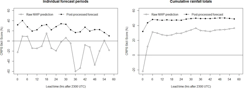
periods. The raw NWP predictions have negative skill for some individual periods, suggesting that it would be better to use a climatology forecast. However, post-processing pro-duces rainfall forecasts with positive skill for all lead times out to 57 h. Forecast skill is highest for rainfall predictions for the 3–6 h lead time and displays a gradual decline with increasing lead time. Post-processing results in marked im-provements in skill over the raw NWP predictions, with the skill of the post-processed forecast being on average 37 % higher than the raw NWP predictions.

The skill of post-processed forecasts of cumulative rainfall totals (Figs. 4 and 5), increases for the first three lead times and then remains relatively stable at a CRPS skill score of ap-proximately 50 % out to 57 h. The raw NWP rainfall predic-tions display similar behaviour, but skill scores are approx-imately 20 % lower than the post-processed forecasts for all lead times. The skill of the cumulative forecasts is greater than forecasts for individual periods because errors in indi-vidual periods will tend to compensate for each other.

Figure 5 presents the skill of the post-processed forecasts conditioned on the forecast mean exceeds a range of thresh-olds ranging between 0 and 5 mm for 0–3 and 30–33 h lead times. The skill of the post-processed forecasts tends to in-crease as the conditioning threshold inin-creases. In parallel, the sample size reduces rapidly and consequently the uncer-tainty of the skill estimates grows. This suggests that the skill of the post-processed forecasts appears to be consistent over the range of thresholds assessed.

4.2.2 Forecast bias

Fig. 3. Observed (red dots) and modelled median (vertical lines,

representing [0.05, 095] uncertainty range) correlation coefficients between NWP forecast and observed precipitation for post-process post-processing models covering lead times from 0 to 57 h at site 82163 Carboor Upper.

developed in a manner that allows for diurnal variations in forecast performance, as done here.

Correction of the forecast bias will be the greatest contri-bution to improvements in forecast skill. Figure 6 displays the correction to the mean bias, however, bias correction us-ing the BJP modellus-ing approach is more sophisticated than just correcting the mean bias. Using different marginal dis-tributions, and particularly transformations, for the raw NWP rainfall predictions and observed data allows for a non-linear bias correction (Fig. 7). This results in improvements in fore-cast skill that are greater than those that would be achieved by just correcting the mean bias.

As expected from the previous analysis, biases in the post-processed cumulative rainfall ensembles are minimal throughout the entire forecast period (Fig. 8). The biases for the raw NWP predictions decrease for lead times up to 9 h and then are relatively stable near zero. However, the mag-nitude of biases in the post-processed ensemble forecasts is nearly always smaller than in the raw forecasts.

The bias of the post-processed forecasts conditioned on the forecast median for 0–3 and 30–33 h lead time forecasts is presented in Fig. 8. The bias begins to depart from close to zero for events where the forecast median exceeds approxi-mately 2.5 mm. However, for nearly all threshold values the confidence limits intersect the black line depicting zero bias and suggesting that the departures from zero may be solely due to sampling uncertainties.

4.2.3 Forecast discrimination

Forecast discrimination is assessed using plots of the rela-tive operating characteristic (ROC). The ability of the post-processed forecasts to discriminate between events and non-events varies with lead time and the event being considered

(Fig. 9). At shorter lead times, the ROC curves for forecasts of individual periods tend to approach the top left corner of the plot, while at longer lead times they are closer to the diag-onal. This suggests that forecasts for shorter lead times have a greater ability to discriminate between events and non-events than forecasts for longer lead times. The contrast in forecast discrimination with lead time is stronger for the high rainfall events (precipitation>5 mm) than for the event of rainfall less than 0.2 mm. This suggests that as lead time increases the probability of high rainfall in the post-processed fore-casts becomes less informative and less strongly correlated observed high rainfall events. However, the ROC curves do not approach the diagonal line at any lead time, which sug-gests the post-processed forecasts are always skilful. This is supported by the skill scores presented earlier.

The ROC curves for cumulative forecast rainfall totals dis-play significantly less spread than the curves for individual forecast lead times. For the event of rainfall less than 0.2 mm, the forecast discrimination is stronger for shorter lead times than for longer lead times. However, for the events of greater than 5 mm, there are no clear differences in forecast discrim-ination with lead time.

Figure 10 presents the area under the ROC curve for a spectrum of event magnitudes for 0–3 and 30–33 h lead times. The area under the ROC curve tends to remain con-stant, given the sampling uncertainty, with increasing event size. This suggests that the skill of the forecasts is not related to the size of the forecast event.

4.2.4 Reliability

Figure 11 presents reliability diagrams for the probability of rainfall exceeding two thresholds for individual forecast lead times pooled for lead times in day 1 and day 2. The reliability diagrams illustrate that the forecast probability of a rainfall event of less than 0.2 mm appears to be reliable, with the ob-served relative frequencies closely following the line reflect-ing perfect reliability. The forecast probability of a rainfall event of greater than 5 mm also appears to be reliable for day 1. For day 2 the forecast probability of a rainfall event of greater 5 mm appears to be less reliable. However, very few forecasts have a probability of rainfall exceeding 5 mm that falls into the upper bin of this diagram, and therefore, there is considerable sampling uncertainty associated with the ob-served frequencies. This sampling uncertainty is highlighted by the wide confidence intervals in Fig. 11.

Fig. 4. Variation in CRPS skill score of ensemble rainfall forecasts for individual periods (left panel) and cumulative rainfall totals (right

panel) with lead time at site 82163 Carboor Upper.

Fig. 5. CRPS skill scores (solid black line) and [0.05, 0.95] confidence intervals (red and blue dashed lines) conditional on the forecast mean

exceeding threshold rainfall for ensemble rainfall forecasts at site 82163 Carboor Upper at lead times of 0–3 h (left panel) and 30–33 h (right panel). The number of events over which the skill scores are computed are given by the black dashed lines.

Overall, the forecasts of 24 h rainfall totals appear to be reli-able.

The probabilistic forecasts of 24 h rainfall totals are pro-duced by summing individual ensemble members. These forecasts will only be reliable if the forecasts for individual periods are reliable and the ensemble members have the ap-propriate temporal correlation structures. The temporal cor-relations in the ensemble members were introduced using the Schaake shuffle. Here we have demonstrated that the probability distributions of forecasts for both individual peri-ods and cumulative totals are reliable and therefore the tem-poral correlations introduced by the Schaake shuffle seem appropriate.

4.2.5 Forecast correlations

Figure 13 presents the lag-1 Kendall correlation of the en-semble rainfall forecasts, before and after application of the Schaake shuffle, and of the corresponding observations. The lag-1 correlations of the probabilistic forecasts before ap-plication of the Schaake shuffle are close to zero, which is

expected given that these forecasts are random samples from independent probability distributions. After application of the Schaake shuffle, the lag-1 correlations of the ensemble forecasts are significantly larger and close to those of the ob-servations. The lag-1 correlations of the ensemble forecasts are expected to be lower than those of the observations be-cause the majority of the forecasts have a larger proportion of zero values than the observations. These zero values will tend to reduce lower magnitude of the correlation coefficients.

5 Further discussion

Fig. 6. Percentage bias for individual forecast lead times (left panel) and cumulative forecast totals (right panel) as a function of lead time at

site 82163 Carboor Upper.

Fig. 7. Ensemble mean plotted against the raw NWP prediction for

lead time 0 forecasts at site 82163 Carboor Upper showing the non-linear nature of bias correction (1 : 1 solid line).

Poorly representing the timing and magnitude of the diurnal cycles, particularly in precipitation, is a known problem with many NWP models and is commonly related to the represen-tation and parameterization of convective processes (Evans and Westra, 2012; Dai and Trenberth, 2004). Therefore, it may be more appropriate to condition the post-processing of NWP rainfall predictions on the type of rainfall rather than lead time. However, previous analysis found that errors in NWP rainfall predictions could not be predicted by synoptic or rainfall types for Australian conditions (Roux et al., 2012). One of the major challenges for developing and evaluating short-term streamflow forecasting systems, and particularly post-processing methods for rainfall predictions, in Australia is the limited availability of retrospective NWP predictions from the ACCESS suite of models. The lack of retrospec-tive NWP predictions imposes some limitations on this study and the conclusions that can be drawn. Significant stream-flow events, including floods, result from significant rainfall

Fig. 8. Percentage bias (solid black line) and [0.05, 0.95] confidence intervals (red and blue dashed lines) conditional on the forecast mean

exceeding threshold rainfall for ensemble rainfall forecasts at site 82163 Carboor Upper at lead times of 0–3 h (left panel) and 30–33 h (right panel). The number of events over which the skill scores are computed are given by the black dashed lines.

Fig. 9. Relative operating characteristics at all lead times for individual forecast lead time and cumulative forecast totals for events of rainfall

less than the minimum observable and events greater than 5 mm at site 82163 Carboor Upper.

for multiple periods from a single model. However, it would require strong parameterization of the correlation matrix to limit the risk of overfitting. Such an approach is attractive as it would remove the need to use the Schaake shuffle to create ensembles from separately post-processed probability distri-butions, as the spatial and temporal correlations would be explicitly modelled. Stronger assumptions about all model parameters may also be able to deal with situations where

little or no rainfall is observed or predicted for some forecast lead times.

Fig. 10. Area under the ROC curve (solid black line) and [0.05, 0.95] confidence intervals (red and blue dashed lines) for a spectrum of

threshold rainfall events for ensemble rainfall forecasts at site 82163 Carboor Upper at lead times of 0–3 h (left panel) and 30–33 h (right panel). The number of events over which the skill scores are computed are given by the black dashed lines.

Fig. 11. Reliability diagrams for the probability of a rainfall event of less than 0.2 mm and the probability of a rainfall event of greater

Fig. 12. Reliability diagrams for the probability of 24 h forecast rainfall totals being less than 0.2 mm and the probability of 24 h forecast

rainfall totals exceeding than 5 mm for day 1 (lead times 0–21 h) and for day 2 (lead times 24–45 h) at site 82163 Carboor Upper (1 : 1 dashed line, perfectly reliable forecast; circles, observed relative frequency; vertical lines, [0.05, 0.95] uncertainty intervals; insert, number of events in each of the different forecast probability ranges).

(Roux and Seed, 2011; Roux et al., 2012). NWP models tend not to predict rainfall from convective systems well because these processes evolve rapidly and commonly occur on spa-tial scales finer than those resolved by the model. In areas where substantial rainfall is produced by convective systems, the raw NWP rainfall predictions may not be sufficiently correlated with rain gauge observations to produce skilful rainfall forecasts using the method described in this paper. Further work is proposed to assess the efficacy of the post-processing method for catchments experiencing a range of climatic conditions in Australia.

The motivation for post-processing NWP rainfall predic-tions is to produce bias free ensemble rainfall forecasts that can be used for ensemble streamflow forecasting. Using bias free ensemble rainfall forecasts to force an initialised hydro-logical model has the potential to increase the number of lead times for which skilful streamflow forecasts can be produced. Assessing the benefits of using ensemble rainfall forecasts for streamflow forecasting is beyond the scope of the current

study, but will be the subject of future investigations. Part of these investigations will include examining the tempo-ral resolution at which post-processed rainfall forecasts are most skilful and which lead to the most skilful streamflow forecasts.

6 Summary and conclusions

Fig. 13. Lag-1 Kendall correlation coefficients for ensemble

fore-casts before and after application of Schaake shuffle and for obser-vations (solid lines, median for all forecast events and observed; shaded bands, [0.05, 0.95] intervals computed from all forecast events).

forecast probability distributions for individual locations and forecast lead times. Ensemble forecasts with appropriate spa-tial and temporal correlations are then generated by linking samples from the forecast probability distributions using the Schaake shuffle.

We apply the approach to post-process rainfall predictions from the ACCESS-R numerical weather prediction model at rain gauge locations in the Ovens catchment in southern Australia. We demonstrate that the assumed log-sinh trans-formed bivariate normal distribution is appropriate for mod-elling the joint distribution of NWP predicted and observed rainfall. The method is shown to produce ensemble forecasts that are more skilful than the raw NWP predictions both for individual forecast lead times and for cumulative forecast to-tals. Skill increases result from the correction of not only the mean bias, but also biases conditional on the magnitude of the NWP rainfall prediction. The post-processed forecast ensembles are demonstrated to successfully discriminate be-tween events and non-events for both small and large rainfall occurrences, and reliably quantify the forecast uncertainty.

This study has assessed the post-processing approach for conditions where rainfall is principally due to large-scale synoptic systems. Further work is proposed to assess the ef-ficacy of the post-processing method for catchments expe-riencing a range of climatic conditions in Australia, particu-larly in areas where significant rainfall is the result of convec-tive processes. Future investigations will also assess the ben-efits of using post-processed rainfall forecasts for flood and short-term streamflow forecasting and examine the temporal resolution at which rainfall post-processing is most effective.

Appendix A

Reparameterization of model parameters

To ease parameter inference, all the parameters of the trans-formed bivariate model are reparameterized. For both the predictor and predictand, the parametersµandσare strongly related to the transformation parameters. These parameters are reparameterized to mands, which are first order Tay-lor series approximations ofµandσ in the untransformed space.

µ= 1

β ln(sinh(α+β m))

σ = 1

tanh(α+β m)s

Further reparameterization of m and s to m∗ and s∗, al-lows for parameter estimation on the entire real space and an approximately linear dependence between the estimated parameters.

m∗=ln

m+ α

β

s∗=2 ln(s)

Logarithms are taken of the two transformation parameters (αandβ). The correlation coefficientris reparameterized to

φusing an inverse hyperbolic tangent or FisherZ transfor-mation (Wang et al., 2009), to give

φ=tanh−1(r).

The collection of parameters used in inference is

θ =

ln(α1) , ln(α2) , ln(β1) , m∗1, m

∗

2, s

∗

1, s

∗

2, ϕ .

Appendix B

Posterior parameter distribution

According to Bayes’ theorem, the posterior distribution of model parameters is

p (θ|YOBS)∝ p(θ) p (YOBS|θ)=p(θ)

Yn

t=1p y t OBS|θ

,

where p(θ ) is the prior distribution representing infor-mation available about parameters before the use of his-torical data and p (YOBS|θ) is the likelihood function defining the probability of observing the historical events YOBS=y1_OBS,y_OBS2 , . . . ,yn_OBSandyt_OBS is the observed predictor and predictand data for event t (t= 1, 2, . . . ,n), given the model and its parameter set.

or equal toa censoring value with an unknown precise value. Formulation of the likelihood functionp (YOBS|θ)allows for general censoring thresholds (yc=y1,c, y2,c ).

The likelihood function is then given by

p(y|θ)

=       

p (y1, y2|θ) =Jz1→y1Jz2→y2p (z1, z2|θ) y1> y1,c, y2> y2,c

p y1< y1,c, y2|θ =Jz2→y2p z1< z1,c, z2|θ y1=y1,c, y2> y2,c p y1, y2< y2,cθ =Jz1→y1p z1, z2< z2,c|θ

y1> y1,c, y2=y2,c p y1< y1,c, y2< y2,c|θ=p z1< z1,c, z2< z2,c|θ y1=y1,c, y2=y2,c ,

where

p z1< z1,c, z2|θ= z1,c Z

−∞

p (z1|z2, θ)dz1×p (z2|θ)

p z1, z2 < z2,c|θ= z2,c Z

−∞

p (z2|z1, θ)dz2×p (z1|θ)

p z1< z1,c, z2< z2,c|θ= z1,c Z −∞ z2,c Z −∞

p (z1, z2|θ)dz1dz2

andzcis the transformed value of the censor threshold cor-responding toyc.

The Jacobian determinant Jz→y of the transformation fromztoy is

Jz→y =

dz

dy =

1 tanh(α+β y).

Appendix C

Prior distribution of parameters

The prior distribution for the model parameters is specified as

p(θ)=Y2

i=1p (lnαi) p (lnβi) p m

∗

i, s

∗

i

p(ϕ).

A uniform prior is specified for both of the transformation parameters; however, because these parameters are not di-rectly estimated it is necessary to apply the Jacobian of the reparameterization to the uniform prior

p(lnα)=Jα→lnαp(α),

where the Jacobian determinant of the reparameterization

(Jα→lnα)is given by

Jα→lnα =

dα

d(lnα) =α

and

p(α)∝1.

Similarly,

p(lnβ)=Jβ→lnβp(β)

where the Jacobian determinant of the reparameterization

Jβ→lnβis given by

Jβ→lnβ =

dβ

d(lnβ) =β

and

p(β)∝ 1.

A more elaborate prior for the pair of(m∗, s∗)is used to deal with the reparameterizations, giving

p m∗, s∗=J_µ,σ2_→m,s2J_s2_→s∗J_m→m∗p

µ, σ2

,

where the Jacobian determinant of the transformation

J_µ,σ2_→m,s2from µ, σ2to m, s2is given by

J_µ,σ2_→m,s2 = ∂µ ∂m ∂µ ∂s2 ∂σ2 ∂m ∂σ2 ∂s2 = ₁

tanh(α+β m)

3 ;

the Jacobian determinant of the reparameterization J_s2_→s∗

froms2tos∗is given by

J_s2→s∗ =

ds2

ds∗ =s

2_;

the Jacobian determinant of the reparameterization (Jm→m∗)

frommtom∗is given by

Jm→m∗ =

dm

dm∗ =m+

α β;

andp µ, σ2

takes the simplest form of priors commonly used for normal distribution mean and variance (Wang and Robertson, 2011; Gelman et al., 1995)

pµ, σ2∝ 1

σ2.

The prior for the reparameterized correlation coefficient is related to the prior for the original correlation coefficient by

p(ϕ)=Jr→ϕp(r),

whereJr→ϕ is the Jacobian determinant for the transform fromrtoϕ, and

Jr→ϕ =

dr

dϕ = [cosh(ϕ)]

−2_.

Wang et al. (2009) use a marginally uniform prior is used for the correlation matrix, which for the bivariate case reduces to

Acknowledgements. This research has been supported by the

Water Information Research and Development Alliance between the Australian Bureau of Meteorology and CSIRO Water for a Healthy Country Flagship and the CSIRO OCE Science Leadership Scheme. We would like to thank David Enever and Chris Leahy from the Australian Bureau of Meteorology for providing the data for this study. We would like to acknowledge the thorough reviews by Andrew Schepen from the Australian Bureau of Meteorology, Jan Verkade and two anonymous referees.

Edited by: F. Pappenberger

References

Australian Bureau of Meteorology: Operational implementation of the ACCESS Numerical Weather Prediction systems, 34, Aus-tralian Bureau of Meteorolgy, Melbourne, 2010.

Blöschl, G.: Flood warning – on the value of local in-formation, Int. J. River Basin Manage., 6, 41–50, doi:10.1080/15715124.2008.9635336, 2008.

Charles, A., Hendon, H. H., Wang, Q. J., Robertson, D. E., and Lim, E.-P.: Comparsion of Techniques for the Calibration of Coupled Model Forecasts of Murray Darling Basin Seasonal Mean Rain-fall, 38, The Centre of Australian Weather and Climate Research, Melbourne, 2011.

Clark, A. J., Kain, J. S., Stensrud, D. J., Xue, M., Kong, F., Coniglio, M. C., Thomas, K. W., Wang, Y., Brewster, K., Gao, J., Wang, X., Weiss, S. J., and Du, J.: Probabilistic Precipitation Forecast Skill as a Function of Ensemble Size and Spatial Scale in a Convection-Allowing Ensemble, Mon. Weather Rev., 139, 1410– 1418, doi:10.1175/2010mwr3624.1, 2011.

Clark, M., Gangopadhyay, S., Hay, L., Rajagopalan, B., and Wilby, R.: The Schaake shuffle: A method for reconstructing space-time variability in forecasted precipitation and tempera-ture fields, J. Hydrometeorol., 5, 243–262, doi:10.1175/1525-7541(2004)005<0243:tssamf>2.0.co;2, 2004.

Dai, A. and Trenberth, K. E.: The Diurnal Cycle and Its Depiction in the Community Climate System Model, J. Climate, 17, 930–951, doi:10.1175/1520-0442(2004)017<0930:tdcaid>2.0.co;2, 2004. Duan, Q., Sorooshian, S., and Gupta, V. K.: Optimal use of the

SCE-UA global optimization method for calibrating watershed mod-els, J. Hydrol., 158, 265–284, 1994.

Ebert, E. E.: Ability of a Poor Man’s Ensemble to Pre-dict the Probability and Distribution of Precipitation, Mon. Weather Rev., 129, 2461–2480, doi:10.1175/1520-0493(2001)129<2461:aoapms>2.0.co;2, 2001.

Evans, J. P. and Westra, S.: Investigating the Mechanisms of Diurnal Rainfall Variability Using a Regional Climate Model, J. Climate, 25, 7232–7247, doi:10.1175/Jcli-D-11-00616.1, 2012.

Gelman, A., Carlin, J. B., Stern, H. S., and Rubin, D. B.: Bayesian data analysis, in: Texts in Statistical Science Series, edited by: Chatfield, C. and Zidek, J. V., Chapman and Hall, London, 526 pp., 1995.

George, B. A., Adams, R., Ryu, D., Western, A. W., Simon, P., and Nawarathna, B.: An Assessment of Potential Operational Bene-fits of Short-term Stream Flow Forecasting in the Broken Catch-ment, Victoria, Proceedings of the 34th IAHR World Congress, Brisbane, Australia, 2011.

Glahn, H. R. and Lowry, D. A.: The Use of Model Out-put Statistics (MOS) in Objective Weather Forecasting, J. Appl. Meteorol., 11, 1203–1211, doi:10.1175/1520-0450(1972)011<1203:tuomos>2.0.co;2, 1972.

Gupta, H. V., Beven, K. J., and Wagener, T.: Model Calibration and Uncertainty Estimation, in: Encyclopedia of Hydrological Sci-ences, John Wiley & Sons Ltd., 2006.

Hamill, T. M. and Colucci, S. J.: Verification of Eta-RSM Short-Range Ensemble Forecasts, Mon. Weather Rev., 125, 1312– 1327, doi:10.1175/1520-0493(1997)125<1312:voersr>2.0.co;2, 1997.

Hamill, T. M., Whitaker, J. S., and Wei, X.: Ensemble Refore-casting: Improving Medium-Range Forecast Skill Using Ret-rospective Forecasts, Mon. Weather Rev., 132, 1434–1447, doi:10.1175/1520-0493(2004)132<1434:erimfs>2.0.co;2, 2004. Hersbach, H.: Decomposition of the continuous ranked

probabil-ity score for ensemble prediction systems, Weather Forecast., 15, 559–570, 2000.

Jolliffe, I. T. and Stephenson, D. B.: Forecast verification : a prac-titioner’s guide in atmospheric science, J. Wiley, Chichester, 240 pp., 2003.

Kleiber, W., Raftery, A. E., and Gneiting, T.: Geostatistical model averaging for locally calibrated probabilistic quantitative precip-itation forecasting, Department of Statistics, University of Wash-ington, Seattle, WA, USZ, 2010.

Pagano, T. C., Ward, P., Wang, X. N., Hapuarachchi, H. A. P., Shrestha, D. L., Anticev, J., and Wang, Q. J.: The SWIFT cal-ibration cookbook: experience from the Ovens, 76, CSIRO, Mel-bourne, 2011.

Penning-Rowsell, E. C., Tunstall, S. M., Tapsell, S. M., and Parker, D. J.: The Benefits of Flood Warnings: Real But Elu-sive, and Politically Significant, Water Environ. J., 14, 7–14, doi:10.1111/j.1747-6593.2000.tb00219.x, 2000.

Pokhrel, P., Robertson, D. E., and Wang, Q. J.: A Bayesian joint probability post-processor for reducing errors and quantifying uncertainty in monthly streamflow predictions, Hydrol. Earth Syst. Sci., 17, 795–804, doi:10.5194/hess-17-795-2013, 2013. Robertson, D. E. and Wang, Q. J.: A Bayesian approach to predictor

selection for seasonal streamflow forecasting, J. Hydrometeorol., 13, 155–171, 2012.

Roulin, E.: Skill and relative economic value of medium-range hy-drological ensemble predictions, Hydrol. Earth Syst. Sci., 11, 725–737, doi:10.5194/hess-11-725-2007, 2007.

Roux, B. and Seed, A. W.: Assessment of the accuracy of the NWP forecasts for significant rainfall events at the scales needed for hydrological prediction, Bureau of Meteorology, Melbourne, 2011.

Roux, B., Seed, A. W., and Dahni, R.: An evaluation of the possibil-ity of correcting the bias in NWP rainfall forecasts, 42, Bureau of Meteorology, Melbourne, 2012.

Santos-Muñoz, D., Martin, M. L., Morata, A., Valero, F., and Pascual, A.: Verification of a short-range ensemble precipita-tion predicprecipita-tion system over Iberia, Adv. Geosci., 25, 55–63, doi:10.5194/adgeo-25-55-2010, 2010.

Shrestha, D. L., Robertson, D. E., Wang, Q. J., Pagano, T. C., and Hapuarachchi, H. A. P.: Evaluation of numerical weather pre-diction model precipitation forecasts for short-term streamflow forecasting purpose, Hydrol. Earth Syst. Sci., 17, 1913–1931, doi:10.5194/hess-17-1913-2013, 2013.

Sloughter, J. M., Raftery, A. E., Gneiting, T., and Fraley, C.: Probabilistic quantitative precipitation forecasting using Bayesian model averaging, Mon. Weather Rev., 135, 3209–3220, doi:10.1175/mwr3441.1, 2007.

Toth, Z., Talagrand, O., Candille, G., and Zhu, Y.: Probability and Ensemble Forecasts, in: Forecast Verification: A Practitioner’s Guide in Atmospheric Science, edited by: Jolliffe, I. T. and Stephenson, D. B., J. Wiley, Chichester, 137–164, 2003. Wang, Q. J. and Robertson, D. E.: Multisite probabilistic forecasting

of seasonal flows for streams with zero value occurrences, Water Resour. Res., 47, W02546, doi:10.1029/2010wr009333, 2011. Wang, Q. J., Robertson, D. E., and Chiew, F. H. S.: A Bayesian

joint probability modeling approach for seasonal forecasting of streamflows at multiple sites, Water Resour. Res., 45, W05407, doi:10.1029/2008WR007355, 2009.

Wang, Q. J., Schepen, A., and Robertson, D. E.: Merging Seasonal Rainfall Forecasts from Multiple Statistical Models through Bayesian Model Averaging, J. Climate, 25, 5524–5537, doi:10.1175/Jcli-D-11-00386.1, 2012a.

Wang, Q. J., Shrestha, D. L., Robertson, D. E., and Pokhrel, P.: A log-sinh transformation for data normalization and variance stabilization, Water Resour. Res., 48, W05514, doi:10.1029/2011wr010973, 2012b.

Wilks, D. S.: Statistical methods in the atmospheric sciences, In-ternational geophysics series, v. 91, Academic Press, Burlington, MA, London, xvii, 627 pp., 2006.

Wu, L., Seo, D.-J., Demargne, J., Brown, J. D., Cong, S., and Schaake, J.: Generation of ensemble precipitation forecast from single-valued quantitative precipitation forecast for hydrologic ensemble prediction, J. Hydrol., 399, 281–298, 2011.