On the colour and spin of epistemic error (and what we might do about it)

www.hydrol-earth-syst-sci.net/15/3123/2011/ doi:10.5194/hess-15-3123-2011

© Author(s) 2011. CC Attribution 3.0 License.

Earth System

Sciences

On the colour and spin of epistemic error

(and what we might do about it)

K. Beven1,2,3, P. J. Smith1, and A. Wood1,4

1_{Lancaster Environment Centre, Lancaster University, Lancaster, UK}

2_{Department of Earth Sciences, Geocentrum, Uppsala University, Uppsala, 75236, Sweden} 3_{Centre for the Analysis of Time Series (CATS), London School of Economics, London, UK} 4_{JBA Consulting, Warrington, UK}

Received: 5 May 2011 – Published in Hydrol. Earth Syst. Sci. Discuss.: 30 May 2011 Revised: 25 August 2011 – Accepted: 26 August 2011 – Published: 13 October 2011

Abstract. Disinformation as a result of epistemic error is an issue in hydrological modelling. In particular the way in which the colour in model residuals resulting from epistemic errors should be expected to be non-stationary means that it is difficult to justify the spin that the structure of residu-als can be properly represented by statistical likelihood func-tions. To do so would be to greatly overestimate the infor-mation content in a set of calibration data and increase the possibility of both Type I and Type II errors. Some princi-ples of trying to identify periods of disinformative data prior to evaluation of a model structure of interest, are discussed. An example demonstrates the effect on the estimated param-eter values of a hydrological model.

1 Introduction

The starting point for this paper is the belief in certain parts of the modeling community that it is necessary to use a statistical framework to evaluate the uncertainty in model predictions. This has been the subject of much discussion in the past, with a range of positions from the pure (even if Bayesian) probabilistic views of, for example, O’Hagan and Oakley (2004), Goldstein and Rougier (2004), Manto-van and Todini (2006), Stedinger et al. (2008) and others, to the sceptical views of Beven (2006) and Andr´eassian et al. (2007). Statistical treatments of errors have been applied quite widely in hydrological modelling, developing from the use of likelihoods based on assumptions about model resid-uals (e.g. Sorooshian and Dracup, 1980) to the much more

Correspondence to: K. Beven

(k.beven@lancs.ac.uk)

sophisticated hierarchical treatments of multiple sources of error exemplified by the BATEA (Kuczera et al., 2006; Thyer et al., 2009; Renard et al., 2010) and DREAM (Vrugt et al., 2008, 2009) methodologies.

There are two main advantages of this approach. The first is that it provides a formal framework underpinned by decades of development of statistical methods, including for example the use of Monte Carlo Markov Chain techniques within a Bayesian framework for evaluating the posterior dis-tributions when new data are added. The second is that it aims to provide an estimate of the probability of predicting an observation conditional on a particular model structure (or structures in Bayesian model averaging) and calibration data set (though note that Bayes original 1763 formulation was not in this form). We will not consider further cases where only forward uncertainty estimation can be carried out. Uncertainty estimates then depend entirely on the prior assumptions about different sources of uncertainty. Condi-tioning on some calibration data makes the problem much more interesting.

modelling process would suggest that the assumptions will be too simplistic.

However, the objectivity claimed for formal statistical methods, in this type of application, lies in the possibility of testing those assumptions against the summary statistics for a particular set of model residuals. It should be good prac-tice in any modelling study to carry out such checks (though this is not often reported in papers based on formal statisti-cal likelihoods). If those assumptions cannot be shown to be valid then, despite the mathematical formalism of the con-sequent inference, there is no objectivity. There may also be some limitations of this kind of objectivity when a num-ber of different sets of assumptions appear to be acceptable, such that a subjective choice between different (formal) er-ror models must be made. In Bayesian statistics there is also the subjective choice of prior distributions that, in some ap-plications, have a significant effect on the resulting posterior distributions. It can also be shown (see for example Beven et al., 2008) that an objective analysis of one data set can lead to erroneous forecasts of new data. This paper discusses one reason why such a situation may arise; the role of epis-temic uncertainties in determining the nature of a series of model residuals. It is suggested that the assumptions of for-mal statistics might be inappropriate in assessing the infor-mation content in such cases. Consequently this may result in misleading inference about model parameters and forecasts.

The main alternative to the formal statistical approach, at least up to now, has been the Generalised Likelihood Uncer-tainty Estimation (GLUE) methodology, first introduced by Beven and Binley (1992). GLUE is consistent with hierar-chical Bayesian methods in that if an error model component is added and the associated likelihood based on formal statis-tical assumptions is used, then the results should be the same (Beven et al., 2007, 2008). However, GLUE also allows in-formal likelihoods (or fuzzy measures) to be used, can treat residual errors implicitly in making predictions, and provides ways of combining likelihoods other than Bayesian multipli-cation, where this seems appropriate. There are some con-ditions under which the resulting posterior likelihoods can be considered as probability distributions (see Smith et al., 2008), but the meaning will be different. When an informal likelihood is used, the resulting predictions will no longer formally be conditional estimates of the probability of pre-dicting an observation, but rather conditional estimates of the probability of a model prediction. This has led to significant criticism of the GLUE method (e.g. Mantovan and Todini, 2006; Stedinger et al., 2008); though both of these critical studies are based on hypothetical examples where the model structure is known to be correct so that there is no epistemic uncertainty (see the extension of one of these cases to an in-correct model structure in Beven et al., 2008).

Experience of using the GLUE methodology with a variety of different likelihood measures suggests that for cases where the ensemble of model predictions can cover the available observations (e.g. in hypothetical examples with a correct

model structure) the resulting estimates of model uncertainty can be rather similar. They will differ more in cases where a model structure is, for whatever reason, biased in part or parts of the calibration in the sense that it is impossible for that model structure to match an observation regardless of choice of parameter values. Some simple error structure, such as constant bias or a simple trend, can be easily handled in a statistical likelihood approach (e.g. Kennedy and O’Hagan, 2001) as can constant heteroscedastic variations in the er-ror variance or a constant autocorrelation function. Time variable changes in bias or variance are more difficult (they suggests that the error series does not have a simple statisti-cal structure) but can be “handled” in the sense of increas-ing the error variance of the identified error model, even in cases when the “best available” (maximum likelihood) model might not actually be fit for purpose, or where the source of the error comes from the poor specification of inputs for one or more events (though note that separating these cases might often be difficult).

In doing so, however, the validity of the model structure as a hypothesis about how the system is functioning will not be questioned. Since the statistical estimates of uncertainty are always conditional on the choice of model(s), there is no inherent testing of the validity of the model as hypothesis. Different models can be tested relative to each other (e.g. by the use of Bayes ratios) but there is no mechanism for total model rejection.

This is different from the GLUE approach which devel-oped out of the earlier Hornberger-Spear-Young (HSY) gen-eralized sensitivity analysis (Hornberger and Spear, 1981). The HSY method investigates the sensitivity of complex sys-tems by differentiating between those models considered to be “behavioural” and those that can be rejected as “non-behavioural”. In that the predictions of model outputs within GLUE are intended to be useful guides to the future out-puts from the system, there is no point in making predictions with models that have not proved to be behavioural in cali-bration. Thus models not thought to be useful in prediction are rejected (or given a likelihood of zero; in the statistical approach a very small likelihood would be given to such a model, but no model would be rejected).

However, this introduces a further degree of subjectivity in GLUE. There is commonly a complete range of behaviours in calibration between models that fit the data well (or as well as might be expected) and those that clearly do not. Thus, deciding on a threshold between what will be considered be-havioural and what will not is necessarily subjective (even if generally common sense will prevail in doing so; see the limits of acceptability approach suggested in Beven, 2006). The effect of this selection can be mitigated to some extent by using an informal likelihood measure that reduces to zero at the rejection limit.

of science is to be as objective as possible, even if the history of science records very many instances of the subjective and selective use of evidence in many different subject areas: the history of using the Hortonian model to explain storm runoff is just such an example in hydrology (see Beven, 2004). We like to have formal frameworks for doing things, in which the consequences follow directly and straightforwardly from the assumptions. So why should we even consider using infor-mal likelihoods and subjectively chosen thresholds? In fact, a somewhat deeper reflection turns that question around. How can we possibly justify the use of statistical error models and formal likelihoods when many of the errors that affect mod-eling uncertainty in hydrology are not “statistical” in nature?

2 Aleatory and epistemic errors

The application of formal statistical methods requires that the representation of errors is fundamentally as random or aleatory variables. Aleatory errors can be represented in terms of the odds (or probabilities) of different outcomes. The original paper of Bayes (1763), for example, was con-cerned with estimating odds on different potential hypothe-ses when there might be some prior (subjective) beliefs about the hypotheses. Bayes equation then provides a formal means for incorporating evidence as represented by a like-lihood function with the subjective prior beliefs to condition a posterior distribution in a way that satisfies the axioms of probability theory.

The issue in the application of Bayes theory to inference about models and their predictions is how to choose a like-lihood function to reflect the evidence contained in a set of model residuals when there are multiple sources of uncer-tainty in the modelling process. Hierarchical Bayesian meth-ods do so by providing a representation of all of the impor-tant sources of uncertainty as aleatory. These representations will then have “hyper-parameters” that are estimated as part of the inference process, based on the series of model residu-als. It is critical to this process, however, that all the sources of error can be treated as if they are aleatory.

This is not, however, the case. Many of the errors that enter into the modelling process are not the result of ran-dom natural variation but the result of a lack of knowledge about processes and boundary conditions. These epistemic uncertainties are, as pointed out in the 1920s by Frank Knight and Maynard Keynes, the “real” uncertainties. They include the poor measurements, the processes that we have left out because they are not deemed to be important (or for which we have no agreed mathematical representation), and the lo-cal catchment characteristics that we cannot know in detail. They also include the “unknown unknowns” that we have not even perceived as being important because of lack of knowl-edge and which therefore are unexpected (and not predicted) when they occur (these are also sometimes referred to as ontological or irreducible uncertainties). We cannot be too

concerned about the latter since past surprises have probably been incorporated into present models and future surprises are difficult to predict. In fact, an ontological uncertainty will become an epistemic uncertainty as soon as it is recog-nised as an issue. We should, however, be directly concerned about the category of epistemic uncertainties, that we can surely perceive but do not know enough about.

3 Colour and spin in epistemic errors

There are very many epistemic errors of this type (see Fig. 1), from spatial patterns of rainfall inputs that vary from storm to storm, to the water equivalent of drifting snow, to radar rain-falls subject to multiple (deterministic) corrections, to rating curve non-stationarities and extrapolations, to evapotranspi-ration fluxes in hetereogeneous terrain. Some of these may be due to natural variability (as well as the limitations of available measurement techniques to observe that variability) but none can be considered as fundamentally aleatory. Such variability will not be “white” but structured or coloured in a variety of ways and it is a significant spin of our under-standing to try to suggest to users of model predictions that they can be treated as if they were aleatory in order to be “objective”.

The general effect of epistemic uncertainty is to make the error characteristics of the variable under study (whether in-put or model residual) to appear structured. If that structure is a well-behaved red noise with stationary characteristics then a statistical model might be found to represent it (e.g. Li et al., 2011). The issue with epistemic error is, however, that it is likely to induce colour that is non-stationary. A classic example is the way in which an error in an input vari-able when processed through a nonlinear model, produces a set of residuals that exhibit bias and autocorrelation that might vary depending on the model structure. That is a logi-cal consequence of the nature of the model dynamics. Since the errors in the inputs are expected to vary from event to event (but not in a random way) that bias and autocorrela-tion will be non-staautocorrela-tionary, and normally gradually reduc-ing in effect over time. The colour will change over time. It is known that in simple statistical inference, the neglect of bias and autocorrelation in error series produces bias in the inferred parameters (e.g. Beven et al., 2008). We should therefore expect the same in more complex cases involving non-stationarity.

Fig. 1. Potential sources of epistemic error in measuring and modelling catchment responses.

significant overestimation (or underestimation) of discharges at flood stages (modellers should be wary of simply accept-ing discharge values provided by monitoraccept-ing Agencies with-out information abwith-out quality control and uncertainties, see Westerberg et al., 2011a). Such errors will not be simply statistical (even where a statistical technique such as regres-sion is used to fit a rating curve to observations). Using any variance-based likelihood function or performance mea-sure that is based on squared residuals (including the Nash-Sutcliffe efficiency measure) might mean that the inference is biased because of just a few periods of such measurements. In rapidly responding catchments timing discrepancies in ei-ther the rainfalls or discharges that affect the apparent timing of the rising limb might also have a significant effect on the apparent residual variance. A timing error in the onset of snow melt can have a persistent effect on the error in model simulations that is specific to that period (e.g. see the exam-ple in Freer et al., 1996).

Distributed models are particularly interesting in respect of epistemic errors. Distributed models allow for model pa-rameters to vary spatially in every solution element (though this is rarely done, and where it has been done by interpo-lation it has not generally been very successful, see Loague et al., 2005). Deeper in the subsurface, distributed models can also allow the geological structure to be reflected in the patterns of parameters. There will be epistemic uncertainty in the detail of that structure and it is usually the case that the choice of a “conceptual model” of the geology (and the first estimates of the associated hydrogeological parameters) is a subjective interpretation based on limited amounts of map and geophysical survey data. This is a case where the epis-temic uncertainty is treated in terms of one or more possible scenarios (see the case study of Refsgaard et al., 2006).

It is, of course, rare that model parameters can be identi-fied for all the solution elements in the discretisation. It is much more common to fix parameters over some part of the domain. This means that local predictions will be in error but because of the complex nonlinear interactions in space between elements and process representations, the effect of this on model residuals will be difficult to quantify. The ef-fect should certainly not, however, be expected to be aleatory, because of the connected, nonlinear, nature of the distributed simulation model. The colour should not, therefore, be ex-pected to be simple in nature.

4 Colour, spin and information content

The reason why this is important is because any colour re-duces the information content of the data that are available. Thus, the inference is likely to be over-conditioned if the colour is neglected or represented as if it was a simple sta-tionary process. The result will be generally poorer perfor-mance in prediction than in calibration because the character-istics of the sources of uncertainty in prediction will be dif-ferent to the calibration data. Epistemic errors are expected to lead to this type of non-stationarity. It is indeed generally accepted in hydrological modelling (and in published results of hydrological models) that performance will be poorer in “validation”, even after “optimisation” of a model in calibra-tion (though it is probably doubtful if many studies where performance is very much poorer in validation actually get published; it is more likely that a further model iteration takes place).

from those in calibration. We can therefore only assume that the characteristics will be in some sense “similar” in predic-tion. In the case of statistical inference, this is to assume that the parameters of the error models fitted in calibration will be constant in prediction (despite the evidence that they might be difficult to identify in calibration, see Beven, 2005 and Beven et al., 2008). In GLUE it is to assume that the like-lihood weights associated with a model parameter set (with its implicit error characteristics) will stay the same in predic-tion. This does not protect against the unexpected (an exam-ple, from the extensively modelled Leaf River data set in the paper by Vrugt et al., 2008, led to the comment of Beven, 2009a).

It is therefore a modelling aphorism that a calibration data set can only be partially informative in the face of epistemic errors. There is no theory of information content to cover such cases. Hence the attraction of spinning the nature of sources of uncertainty to suggest that they can be treated as

if they were aleatory. Statistical inference does provide a

theory of information content. Classical Gaussian theory, for example, allows individual residual errors to contribute to the likelihood function as:

L ∝ exp−ρt e2t

(1) whereet is the residual error at time t. amd ρt a scaling factor. In the simplest case of an error model that can be as-sumed to be zero mean and Gaussian with no autocorrelation, this leads to the likelihood function:

Y

t 1 √

2π σ exp

− 1

2σ2 e 2 t

(2)

whereσ2is the residual variance. In this framework every residual is considered to be informative (albeit with contri-butions that can be weighted according toρt). Indeed some hydrological modellers would require this to be the case (e.g. Mantovan and Todini, 2006) for the inference to be “co-herent” (see also the response of Beven et al., 2008). The smaller the error, the higher the contribution, but the multi-plicative effect over a large number of time steps is to pro-duce a highly peaked likelihood surface, with the danger therefore that where the assumptions of the error model on which the likelihood function is based are not correct (Eq. 2 would not be appropriate for the autocorrelated residuals of most hydrological models, for example), then the contribu-tion to the informacontribu-tion content of individual residuals is be-ing overestimated.

As Tarantola (2005) for example points out, the assump-tion in Eq. (1) is subjective (see also Beven, 2002, 2009b). It is not the only choice about how far a residual contributes information to the conditioning process. Laplace (1774) for example developed an alternative theory based on the abso-lute values of residuals, i.e.:

L ∝ exp(−|ρt et|). (3)

Since this was mathematically less tractable, it was largely dropped in favour of the Gaussian measure. But neither is a truly objective assessment of information content. They are only objective within the context of the basic assumptions of Eqs. (1) and (3). This applies also to other error norms, or subjective choices of likelihood, that might be chosen.

Such measures should therefore be treated more as hy-potheses about future performance to be tested. Statistical er-ror models then provide a formal expectation of performance (in terms of the probability of predicting a future observation) that can be evaluated in terms of actual performance (e.g. in terms of quantile-quantile plots for new prediction periods). Models chosen on the basis of subjective likelihood measures do not have such a probabilistic expectation (as noted earlier, the interpretation of the resulting uncertainty bounds is dif-ferent). There is an assumption, however, that the character-istics of the errors in prediction should be “similar” to those seen in calibration (see, for example, Liu et al., 2009). Such an assumption can be tested in a similar way. Departures from the range of model predictions (in both calibration and prediction periods) might be useful in identifying consistent model structural error or non-stationary epistemic error (see, for example, Westerberg et al., 2011b).

There is no real reason why a more direct recognition of epistemic errors should not be based on choices about in-formation content in a way that allows for the expectation of future variability in error characteristics. The difficulty in doing so is that epistemic errors are those for which, by definition, we have little or no information about their na-ture in calibration and even less about the potential errors in prediction.

What we can do, however, is list some desirable qualities or principles for an assessment of information content when we suspect that the modelling process is subject to structural error. These should then be reflected in any model evalua-tion and likelihood assessment. In their strongest form these principles might be expressed as:

1. Information should be assessed so as to minimise, as far as possible, Type I (false positive, or accepting a model that would not provide useful predictions) and Type II (false negative, or rejecting a model that would provide useful prediction) errors.

2. Periods of disinformative inputs or outputs should be identified as far as possible independently of any model structure to avoid the reductio ad absurdum of all peri-ods that do not fit a particular model being rejected as disinformative.

3. Contributions to model likelihood evaluations should be a function of the time varying information content of the observations.

These features may be desirable but will be difficult to sat-isfy because of the expectation that the epistemic errors will be non-stationary and of complex structure, while principle 2 precludes the use of model residuals in assessing informa-tion content in this sense. It is difficult therefore to define a strategy for the independent estimation of such errors with-out additional information being provided (which generally is not possible for periods of past calibration data).

5 Avoiding false negatives

The first principle above is important. It is a fundamental principle for the assessment of information content. It is worth noting, however, that false negative errors are much more important than false positives. The potential for false positives is the reason underlying principle 2, but false posi-tives will generally be less serious because they can be cor-rected as more information becomes available. However, once a model that would provide useful predictions in the future is rejected (a false negative), those useful predictions will not then be available. There is little experience in testing hydrological models as hypotheses within such a framework (Beven, 2010).

False positive and false negative inferences can be ex-pected to result when the driving data for a model are hydro-logically inconsistent with the observed variables with which model simulated variables will be compared. We might ex-pect such an inconsistency to be expressed in terms of large model residuals (even for a model that might be useful in prediction) but, following principle 2, we would ideally wish to assess consistency independently of the model hypothesis being evaluated.

So what does hydrological consistency mean? That the in-puts and outin-puts should be consistent with the mass, energy and momentum balances and what is known about the pro-cesses in a catchment. But these are difficult to assess. As part of the Representative Elementary Watershed concepts, Reggiani and Schellekens (2003, see also Reggiani et al., 2000, 2001) have shown that the mass, energy and momen-tum balances can be expressed for catchment or subcatch-ment units but that they are subject to an important closure problem. Expressed in terms of the simplest lumped catch-ment water balance for example, we can classically write: Q = R +E +1S

whereQis discharge, P is all types of precipitation,E is evapotranspiration rate and1Sis the integral change in stor-age for all points and at all levels in the catchment. In fact, even this is too simplistic, since there may be unmeasured discharges,U, from a catchment (due to regional groundwa-ter fluxes, or unmeasured subsurface fluxes beneath a gaug-ing site). Thus:

Q = R +E +1S +U

In addition each of these terms would be subject to estimation errors, particularly over short periods of time (such as those for which we might wish to assess the information content of data). Allowing for such uncertainties in observed val-ues of the variables is, in general and even for experimental catchments, the only way in which the water balance can be closed. In practice, therefore, inconsistencies can only be as-sessed in the broadest sense of departures from the behaviour seen in the data series as a whole.

In keeping with principle 2 therefore, is there a way of identifying periods of inconsistent data independent of any model structure being evaluated? Two strategies (at least) would seem feasible. One is to use a non-parametric method for explaining relationships in the observations themselves, such as the regression tree methodology used by Iorgulescu and Beven (2004). Past experience suggests that this can be useful in identifying anomalous periods of data. The sec-ond would be to identify a characteristic response function for a catchment (the unit hydrograph) and test for anomalies in runoff coefficients for individual storms (allowing for the antecedent state of the catchment and seasonal effects in the form of accumulated evapotranspiration since the previous event).

There are dangers in both of these approaches, in that “un-usual” periods in the observations, if they were in fact hydro-logically consistent, would probably be the most informative in differentiating between model hypotheses. There is there-fore a need to differentiate between hydrologically consistent and hydrologically inconsistent anomalies (with analogous possibilities of being wrong as a result of uncertainty). Re-member, however, that we should expect not to be sure about identifying hydrological inconsistencies in all cases. There will always be the potential for making Type I and Type II errors.

More generally, principle 3 suggests that it might be possi-ble to rank observations or periods of observations in terms of their contribution to total information content in conditioning a model. This implies a more continuous scale of information than simply excluding certain periods of data considered to be disinformative. Such a ranking, or weighting, of different periods of data might be expected to be context dependent, with relevance to the particular type of application of interest and to the expected observation errors (the classical statisti-cal weighting as an inverse function of observation variance is an example of this). It is also the case that the same set of observations might have more information content with respect to one model output or component than to another. There has been some (limited) exploration of this concept al-ready in hydrological modelling, with Gupta et al. (2008); Wagener et al. (2003).

might be compromised by input uncertainties that, in many cases, are very difficult to characterise because of hetero-geneities and non-stationarities between events. It was this type of uncertainty that was the issue at the heart of the dis-cussion between Beven (2009a) and Vrugt et al. (2008, 2009) and that was illustrated by Beven and Westerberg (2011).

6 An example

The above points can be illustrated by considering an exam-ple, the calibration of a rainfall-runoff model to observed data. The observed data are those readily available in the UK, discharges from an Environment Agency stream gauge and hourly rainfall totals from Met Office rain gauges. The catchment is the South Tyne station 23006 at Featherstone (322 km2). This catchment is predominantly moorland veg-etation and the land-use is mainly for rough grazing. The geology is mainly Carboniferous limestone. An important consideration for the choice of this catchment was that the flows for this site are natural to within 10 % at the 95 per-centile flow. Five recording rain gauges are available within the catchment boundary of the chosen site, with catchment average rainfalls being estimated using a Thiessen polygon method. Comparison with storage gauges in the catchment revealed that the recording gauges generally estimated higher rainfall totals than the storage gauges. There is scope for both the under and overestimation of the inputs to the catchment under different rainfall patterns.

Discharges are measured using a compound Crump weir, which contains the flow at all stages and remains modular throughout its range. There is some suspicion of truncation of higher peaks, possibly due to stilling well problems, but the discharge data are generally considered to be of good quality and are included in the UK HiFlows database.

Periods of disinformative data were assessed though the use of event runoff coefficients. Variability in event runoff coefficients is to be expected due to inadequacies in observ-ing both the precipitation input and the output discharge as well as differing internal states of the system. However, events whose runoff coefficients differ substantially from similar events (e.g. those with similar rainfall totals falling in the same season) should be further investigated. In some cases these may be examples of catchment dynamics not of-ten observed so should remain in the analysis; in other cases they may be disinformative.

6.1 Selection of disinformative periods

To perform the selection of disinformative data periods on an event basis, the observed data needs to be broken into events for which the total runoff and precipitation can be computed. Calculating the total runoff requires the extrapolation of the falling limb of the event hydrograph to estimate the volume

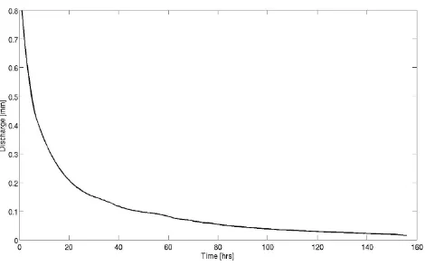
Fig. 2. Plot of the lower part of the master recession curve.

of discharge that might have been observed if further rainfall had not occurred.

The analysis of recession curves has a long history in hy-drology and extensive reviews have been provided by Hall (1968) and Tallaksen (1995). In spite of well-known dif-ficulties with recession variability and partitioning of flow sources, an analysis of recession curves can often give some indication of the characteristics of the subsurface discharges from a catchment and can be used to develop catchment stor-age models (Lamb and Beven, 1997).

The approach taken for this study was to develop a master recession curve (MRC) by piecing together individual shorter recession curves. Ideally, only true flow recessions should be selected where there is no rainfall and minimal evapotran-spiration during the flow recession period. In practise this ideal is difficult to achieve and in this study the MRC was constructed by piecing together individual recession curves of greater than 12 h duration during which less then 0.2 mm of rainfall fell. Figure 2 shows the lower part of the MRC.

Table 1. Table showing the number of Monte Carlo samples considered behavioural for varying thresholds. Values for the data series with

disinformative periods removed are shown in brackets.

κmin κmax

1 0.99 0.98 0.97 0.95 0.93

−100 10 152 (10 192) 5819 (9544) 456 (6082) 145 (2968) 22 (1408) 1 (789)

−50 8733 (8754) 4885 (8201) 333 (5213) 111 (2561) 16 (1175) 1 (641)

−30 7459 (7478) 4095 (7011) 235 (4442) 81 (2181) 12 (977) 1 (507)

−10 4192 (4214) 2210 (3920) 86 (2471) 25 (1262) 2 (496) 0 (215)

−5 2276 (2308) 980 (2090) 13 (1162) 6 (549) 1 (164) 0 (56)

Fig. 3. Schematic showing the calculation of the runoff volume

as-sociated with an event. The lighter shaded area represents the runoff volume associated with the event which starts at time 0 and the darker shaded area an underlying baseflow The subsequent events starts after 67 h (solid line) so the lighter shaded area after this time is extrapolated using the MRC.

accepted (the mean runoff coefficient over the whole period in this catchment is 0.8).

6.2 Influence of disinformative data on calibration

Consider calibrating a lumped hydrological model to the ob-served flow series. The effects of the disinformative data on the calibration of a hydrological model can be illustrated using the lumped rainfall runoff model outlined in Eqs. (4) and (5). The model is Hammerstein in form representing a non-linear transform of the input rainfall series (Eq. 4) and then routing through two parallel tanks expressed as a linear transfer function. The linear transfer function is as-sumed to be mass conservative so that the parameterisation (α1, α2, β1, β2)can be simplified to(α1, α2, ρ)whereρis the split fraction of effective input entering the first path. To ensure the model is physically meaningful(α1, α2, ρ, φ1) lie between 0 and 1, whileφ2is greater than 0 (the range 0 to 2 is considered). To ensure identifiability the condition α2> α1is imposed.

Fig. 4. Scatter plot of runoff coefficient against total rainfall for the

1817 events identified in the time period. Those in red are consid-ered as disinformative.

ut = φ2ytφ1 rt (4)

xt = β1 1 −α1

ut−2 + β2 1− α2

ut−2 (5)

Twelve thousand uniformly distributed random samples were drawn from the parameter ranges outlined above. For each parameter set the maximum and minimum values of the scaled residual(yt−xt)/yt were computed for: (a) the first 900 events identified in the time series and (b) those events in the first 900 that are not excluded as disinformative. Pa-rameter sets were considered behavioural if

min t

yt −xt yt

> κmin

and max

t

yt −xt yt

< κmax.

Fig. 5. Cumulative distribution ofφ1for behavioural parameter sets

of the two situations considered: Analysis using the full data set with(κ_min, κmax)= (−10, 0.98) (solid) and with the disinformative

data removed with(κmin, κmax)= (−5, 0.93) (dot-dash).

that the model which is not considered behavioural for say (κmin, κmax)= (−10, 0.98) may be considered behavioural for stricter conditions (e.g. (κmin, κmax)= (−10, 0.9) when the disinformative data is removed.

Specification of the behavioural threshold can therefore affect the potential for making Type II errors, but specify-ing too generous a bound will also increase the possibility of Type I errors. To illustrate how these trade-offs may influ-ence the conclusions drawn from analysis of the model two situations are contrasted. Situation 1 relates to considering the full calibration data set and specifying behavioural limits of(κmin, κmax)= (−10, 0.98). The second situation consid-ers analysis using only the informative data and behavioural thresholds of(κmin, κmax)= (−5, 0.93).

Figures 5 and 6 show that the resulting distribution of the behavioural parameters sets may change both in location and spread. Figure 7 shows how the selection of the threshold may influence the output of the behavioural model simula-tions for several events outside the calibration period. The simulation results indicate that the very simple model used is structurally deficient, failing to capture the changes in timing in the rising limb of the hydrograph while tending to over-estimate the peak discharge.

7 Back to the unexpected future

In calibration, therefore, we can attempt to identify periods of data that might be disinformative in model inference inde-pendent of model runs. We should not expect a behavioural model to predict such periods of data (while recognising that we might still be making Type I errors in accepting some models as behavioural). There might be similar periods of hydrologically inconsistent data in prediction, that can be identified in similar ways to those applied in calibration. It therefore follows that we should not expect such periods to

Fig. 6. Cumulative distribution ofα2for behavioural parameter sets

of the two situations considered: Analysis using the full data set with(κmin, κmax)= (−10, 0.98) (solid) and with the disinformative

data removed with(κmin, κmax)= (−5, 0.93) (dot-dash).

Fig. 7. Simulation results for an event not within the calibra-tion period. the shaded area represents the limits (evaluated on a time step by time step basis) of the simulations deemed to be behavioural when calibrated against all the calibration data with (κmin, κmax)= (−10,0.98). The lines correspond to

the limits when on the informative calibration data is used and

(κmin, κmax)= (−5, 0.93).Points represent the observed data.

be well predicted by the set of behavioural models identified in calibration. We should also not expect that such periods would be covered by any statistical representation of the cal-ibration errors, since the epistemic uncertainties of inconsis-tent periods in prediction might be quite different to those in calibration. The only response to this would appear to be to moderate our expectations of what a model, or set of models, can do in prediction.

We might expect the uncertainty in the driving variables for hydrological and hydraulic models to be reduced by the application of new or more pervasive measurement tech-niques into the future. The next generation of radar estimates of rainfalls or satellite estimates of surface soil moisture will, we are assured, provide greater accuracy and finer resolu-tion. It might still be expected, however, that some significant epistemic uncertainties in model inputs and model structures will remain for the foreseeable future.

We think we have a pretty good perceptual model of how catchment systems work such that many of the epistemic certainties discussed above arise, not from unperceived un-knowns, but from the limitations of current measurement techniques, spatial and temporal sampling, estimating ef-fective parameter values etc. But, of course, this is true for every generation, and then some unexpected information comes along to change that impression. For the early com-puter modelling generation, one of the most important unex-pected pieces of information was the introduction of tracer data that allowed the residence times in catchments to be addressed in ways not previously possible (e.g. Sklash and Farvolden, 1979). Suddenly, subsurface flows could not be ignored (see also the history of the R5 modelling exercise reported in Loague and Vanderkwaak, 2002 and modelling the Plynlimon chloride data in Kirchner et al., 2001 and Page et al., 2007).

What we can be sure of is that the next generation of hy-drological modellers will also have access to new and bet-ter geophysical and geochemical information, and that their perceptions of how hydrological systems work will change. There remain some epistemological uncertainties of which, as yet, we have only the vaguest intimation but which we should expect to be reduced in achieving better hydrological simulations and improved integrated catchment management in the future.

8 Conclusions

Disinformation as a result of epistemic error is an issue in hydrological modelling. In particular the way in which the colour in model residuals resulting from epistemic errors should be expected to be non-stationary means that it is dif-ficult to justify the spin that the structure of residuals can be properly represented by statistical likelihood functions. To do so would be to greatly overestimate the information con-tent in a set of calibration data and increase the possibility of both Type I and Type II errors. This has been recognised in the past in the bias to be expected in posterior parame-ter distributions when too simplistic a likelihood function is used, but it has been suggested here that the problem is much more significant. Some techniques have been suggested for identifying periods of disinformative data prior to evaluation of a model structure of interest, and the effect on the esti-mated parameter values of a hydrological model has been demonstrated.

Acknowledgements. This work has been funded by the EPSRC

Flood Risk Management Research Consortium project and the EU IMPRINTS FP7 project. We thank both Alberto Montanari and Andras Bardossy for their thoughtful and valuable referee comments and Ida Westerberg for her perceptive suggestions. Edited by: T. Moramarco

References

Andr´eassian, V., Lerat, J., Loumagne, C., Mathevet, T., Michel, C., Oudin, L., and Perrin, C.: What is really undermining hydrologic science today?, Hydrol. Process., 21, 2819–2822, 2007. Bayes, T.: An essay towards solving a problem in the doctrine of

chances, Philos. T. Roy. Soc. Lond., 53, 370–418, 1763. Beven, K. J.: Towards a coherent philosophy for modelling the

en-vironment, P. Roy. Soc. Lond. A, 458, 2465–2484, 2002. Beven, K. J.: Robert E. Horton’s perceptual model of infiltration

processes, Hydrol. Process., 18, 3447–3460, 2004.

Beven, K. J.: On the concept of model structural error, Water Sci. Technol., 52, 165–175, 2005.

Beven, K. J.: A manifesto for the equifinality thesis, J. Hydrol., 320, 18–36, 2006.

Beven, K. J.: Comment on “Equifinality of formal (DREAM) and informal (GLUE) Bayesian approaches in hydrologic model-ing?” by Jasper A. Vrugt, Cajo J. F. ter Braak, Hoshin V. Gupta and Bruce A. Robinson, Stoch. Environ. Res. Risk Assess., 23, 1059–1060, 2009a.

Beven, K. J.: Environmental Modelling: An Uncertain Future?, Routledge, London, UK, 2009b.

Beven, K. J.: Preferential flows and travel time distributions: defin-ing adequate hypothesis tests for hydrological process models Preface, Hydrol. Process., 24, 1537–1547, 2010.

Beven, K. J. and Binley, A. M.: The Future of Distributed Models – Model Calibration and Uncertainty Prediction, Hydrol. Process., 6, 279–298, 1992.

Beven, K. J. and Westerberg, I.: On red herrings and real herrings: disinformation and information in hydrological inference, Hy-drol. Process., 25, 1676–1680, doi:10.1002/hyp.7963, 2011. Beven, K. J., Smith, P. J., and Freer, J.: Comment on “Hydrological

forecasting uncertainty assessment: incoherence of the GLUE methodology” by Pietro Mantovan and Ezio Todini, J. Hydrol., 338, 315–318, 2007.

Beven, K. J., Smith, P. J., and Freer, J.: So just why would a mod-eller choose to be incoherent?, J. Hydrol., 354, 15–32, 2008. Buytaert, W. and Beven, K. J.: Regionalization as a

learning process, Water Resour. Res., 45, W11419, doi:10.1029/2008WR007359, 2009.

Freer, J., Beven, K. J., and Ambroise, B.: Bayesian estimation of uncertainty in runoff prediction and the value of data: An ap-plication of the GLUE approach, Water Resour. Res., 32, 2161– 2173, 1996.

Goldstein, M. and Rougier, J.: Probabilistic formulations for trans-ferring inferences from mathematical models to physical sys-tems, Siam J. Sci. Comput., 26, 467–487, 2004.

Hall, F. R.: Base-flow Recessions-a Review, Water Resour. Res., 4, 973–983, doi:10.1029/WR004i005p00973, 1968.

Hornberger, G. M. and Spear, R. C.: An Approach To the Preliminary-analysis of Environmental Systems, J. Environ. Manage., 12, 7–18, 1981.

Iorgulescu, I. and Beven, K. J.: Nonparametric direct mapping of rainfall-runoff relationships: An alternative approach to data analysis and modeling?, Water Resour. Res., 40, W08403, doi:10.1029/2004WR003094, 2004.

Kennedy, M. C. and O’Hagan, A.: Bayesian calibration of computer models, J. Roy. Stat. Soc. B, 63, 425–450, 2001.

Kirchner, J. W., Feng, X. H., and Neal, C.: Catchment-scale advec-tion and dispersion as a mechanism for fractal scaling in stream tracer concentrations, J. Hydrol., 254, 82–101, 2001.

Kuczera, G., Kavetski, D., Franks, S., and Thyer, M.: Towards a Bayesian total error analysis of conceptual rainfall-runoff mod-els: Characterising model error using storm-dependent parame-ters, J. Hydrol., 331, 161–177, 2006.

Lamb, R. and Beven, K.: Using interactive recession curve analysis to specify a general catchment storage model, Hydrol. Earth Syst. Sci., 1, 101–113, doi:10.5194/hess-1-101-1997, 1997.

Laplace, P.: M´emoire sur la probabilit´e des causes par les ´ev`enements, M´emoires de l’Academie de Science de Paris, 6, 621–656, 1774.

Li, L., Xu, C.-Y., Xia, J., Engeland, K., and Reggiani, P.: Uncer-tainty estimates by Bayesian method with likelihood of AR (1) plus Normal model and AR (1) plus Multi-Normal model in dif-ferent time-scales hydrological models, J. Hydrol., 406, 54–65, doi:10.1016/j.jhydrol.2011.05.052, 2011.

Liu, Y., Freer, J. E., Beven, K. J., and Matgen, P.: Towards a lim-its of acceptability approach to the calibration of hydrological models: extending observation error, J. Hydrol., 367, 93–103, doi:10.1016/j.jhydrol.2009.01.016, 2009.

Loague, K. and Vanderkwaak, J. E.: Simulating hydrological re-sponse for the R-5 catchment: comparison of two models and the impact of the roads, Hydrol. Process, 16, 1015–1032, 2002. Loague, K., Heppner, C. S., Abrams, R. H., Carr, A. E.,

VanderK-waak, J. E., and Ebel, B. A.: Further testing of the Integrated Hydrology Model (InHM): event-based simulations for a small rangeland catchment located near Chickasha, Oklahoma, Hydrol. Process., 19, 1373–1398, 2005.

Mantovan, P. and Todini, E.: Hydrological forecasting uncertainty assessment: Incoherence of the GLUE methodology, J. Hydrol., 330, 368–381, 2006.

O’Hagan, A. and Oakley, J. E.: Probability is perfect, but we can’t elicit it perfectly, Reliabil. Eng. Syst. Saf., 85, 239–248, 2004. Page, T., Beven, K. J., Freer, J., and Neal, C.: Modelling the

chlo-ride signal at Plynlimon, Wales, using a modified dynamic TOP-MODEL incorporating conservative chemical mixing (with un-certainty), Hydrol. Process., 21, 292–307, 2007.

Refsgaard, J. C., van der Sluijs, J. P., Brown, J., and van der Keur, P.: A framework for dealing with uncertainty due to model structure error, Adv. Water Res., 29, 1586–1597, 2006.

Reggiani, P. and Schellekens, J.: Modelling of hydrological re-sponses: the representative elementary watershed approach as an alternative blueprint for watershed modelling, Hydrol. Process., 17, 3785–3789, 2003.

Reggiani, P., Sivapalan, M., and Hassanizadeh, S. M.: Conservation equations governing hillslope responses: Exploring the physical basis of water balance, Water Resour. Res., 36, 1845–1863, 2000. Reggiani, P., Sivapalan, M., Hassanizadeh, S. M., and Gray, W. G.: Coupled equations for mass and momentum balance in a stream network: theoretical derivation and computational experiments, P. Roy. Soc. Lond. A, 457, 157–189, 2001.

Renard, B., Kavetski, D., Kuczera, G., Thyer, M., and Franks, S. W.: Understanding predictive uncertainty in hydrologic mod-eling: The challenge of identifying input and structural errors, Water Resour. Res., 46, W05521, doi:10.1029/2009WR008328, 2010.

Sklash, M. G. and Farvolden, R. N.: Role Of Groundwater In Storm Runoff, J. Hydrol., 43, 45–65, 1979.

Smith, P., Beven, K. J., and Tawn, J. A.: Informal likelihood mea-sures in model assessment: Theoretic development and investi-gation, Adv. Water Resour., 31, 1087–1100, 2008.

Sorooshian, S. and Dracup, J. A.: Stochastic Parameter-Estimation Procedures For Hydrologic Rainfall-Runoff Models - Correlated And Heteroscedastic Error Cases, Water Resour. Res., 16, 430– 442, 1980.

Stedinger, J. R., Vogel, R. M., Lee, S. U., and Batchelder, R.: Appraisal of the generalized likelihood uncertainty esti-mation (GLUE) method, Water Resour. Res., 44, W00B06, doi:10.1029/2008WR006822, 2008.

Tallaksen, L. M.: A Review of Baseflow Recession Analysis, J. Hydrol., 165, 349–370, 1995.

Tarantola, A.: Inverse problem theory and model parameter estima-tion, SIAM, Philadelphia, PA, 2005.

Thyer, M., Renard, B., Kavetski, D., Kuczera, G., Franks, S. W., and Srikanthan, S.: Critical evaluation of parameter consistency and predictive uncertainty in hydrological modeling: A case study using Bayesian total error analysis, Water Resour. Res., 45, W00B14, doi:10.1029/2008WR006825, 2009.

Vrugt, J. A., ter Braak, C., Gupta, H. V., and Robinson, B.: Equi-finality of formal (DREAM) and informal (GLUE) Bayesian ap-proaches in hydrologic modeling?, Stoch. Environ. Res. Risk As-sess., 23, 1011–1026, doi:10.1007/s00477-008-0274-y, 2008. Vrugt, J. A., ter Braak, C. J. F., Gupta, H. V., and Robinson, B. A.:

Response to comment by Keith Beven on “Equifinality of for-mal (DREAM) and inforfor-mal (GLUE) Bayesian approaches in hydrologic modeling?”, Stoch. Environ. Res. Risk Assess., 23, 1011–1026, doi:10.1007/s00477-008-0274-y, 2009.

Wagener, T., McIntyre, N., Lees, M. J., Wheater, H. S., and Gupta, H. V.: Towards reduced uncertainty in conceptual rainfall-runoff modelling: Dynamic identifiability analysis, Hydrol. Process., 17, 455–476, 2003.

Westerberg, I., Guerrero, J. L., Seibert, J., Beven, K. J., and Halldin, S.: Stage-discharge uncertainty derived with a non-stationary rat-ing curve in the Choluteca River, Honduras, Hydrol. Process., 25, 603–613, 2011a.