Introducing empirical and probabilistic regional envelope curves into a mixed bounded distribution function

www.hydrol-earth-syst-sci.net/14/2465/2010/ doi:10.5194/hess-14-2465-2010

© Author(s) 2010. CC Attribution 3.0 License.

Earth System

Sciences

Introducing empirical and probabilistic regional envelope curves

into a mixed bounded distribution function

B. Guse1,2,*_{, Th. Hofherr}2,3,4_{, and B. Merz}1

1_{Deutsches GeoForschungsZentrum Potsdam GFZ, Section 5.4 – Hydrology, Telegrafenberg, 14473 Potsdam, Germany} 2_{Center for Disaster Management and Risk Reduction Technology (CEDIM), 76187 Karlsruhe, Germany}

3_{Institute for Meteorology and Climate Research, Karlsruhe Institute of Technology (KIT), 76128 Karlsruhe, Germany} 4_{Geo Risks Research, M¨unchener R¨uckversicherungs-Gesellschaft, 80791 Munich, Germany}

*_{now at: Department of Hydrology and Water Resources Management, Christian-Albrechts-Universit¨at zu Kiel,} Olshausenstrasse 40, 24098 Kiel, Germany

Received: 3 June 2010 – Published in Hydrol. Earth Syst. Sci. Discuss.: 6 July 2010 Revised: 3 November 2010 – Accepted: 16 November 2010 – Published: 9 December 2010

Abstract. A novel approach to consider additional spatial information in flood frequency analyses, especially for the estimation of discharges with recurrence intervals larger than 100 years, is presented. For this purpose, large flood quan-tiles, i.e. pairs of a discharge and its corresponding recur-rence interval, as well as an upper bound discharge, are com-bined within a mixed bounded distribution function. The large flood quantiles are derived using probabilistic regional envelope curves (PRECs) for all sites of a pooling group. These PREC flood quantiles are introduced into an at-site flood frequency analysis by assuming that they are represen-tative for the range of recurrence intervals which is covered by PREC flood quantiles. For recurrence intervals above a certain inflection point, a Generalised Extreme Value (GEV) distribution function with a positive shape parameter is used. This GEV asymptotically approaches an upper bound de-rived from an empirical envelope curve. The resulting mixed distribution function is composed of two distribution func-tions which are connected at the inflection point.

This method is applied to 83 streamflow gauges in Sax-ony/Germany. Our analysis illustrates that the presented mixed bounded distribution function adequately considers PREC flood quantiles as well as an upper bound discharge. The introduction of both into an at-site flood frequency ysis improves the quantile estimation. A sensitivity anal-ysis reveals that, for the target recurrence interval of 1000

Correspondence to: B. Guse ([email protected])

years, the flood quantile estimation is less sensitive to the se-lection of an empirical envelope curve than to the sese-lection of PREC discharges and of the inflection point between the mixed bounded distribution function.

1 Introduction

Flood frequency analysis provides flood quantiles, i.e. dis-charges and their corresponding recurrence intervals. Espe-cially for recurrence intervalsT >100 years, flood quantile estimates are very uncertain, due to the limited length of the measured flood series and the low number of representative data for extreme floods (e.g. Cohn and Stedinger, 1987; Merz and Thieken, 2005; Reis Jr. and Stedinger, 2005).

of extreme floods and therefore to describe the upper tail be-haviour of a distribution function.

Second, systematic time series can be extended by inte-grating historic floods as non-systematic data (Stedinger and Cohn, 1986). These historic extreme floods lead to more data for the estimation of large quantiles (e.g. England Jr. et al., 2003b; Benito et al., 2004). Historic observations con-tain considerable measurement errors, but due to the short systematic observation period, such additional information is useful (e.g. Hosking and Wallis, 1986b), and an increase of the effective record length leads to a better estimation of flood quantiles (Condie and Lee, 1982; Stedinger and Cohn, 1986; Cohn and Stedinger, 1987).

Third, flood regionalisation aims at improving flood quan-tile estimates by using information from gauges with similar hydrologic characteristics. In this way, the limited length of flood series is compensated by using regional flood series, following the principle of “trading space for time” (Stedinger et al., 1993). Gutknecht et al. (2006) proposed to combine lo-cal and regional methods within a “multi-pillar”-approach to reduce the uncertainty of flood quantile estimates for large recurrence intervals.

The selection of a distribution function which is suitable to estimate extreme floods is difficult (e.g. Merz and Thieken, 2005; El Adlouni et al., 2008). Parameter estimation meth-ods mostly concentrate on the central parts of the distribution function. The upper tail which is the most relevant for ex-treme flood events and is subject to the largest uncertainty is often not adequately described (Moon et al., 1993). Hence, for the estimation of large flood quantiles, it is recommended to concentrate on extreme floods and to derive as much in-formation as possible from them (Naghettini et al., 1996).

Hydrological characteristics, e.g. generation mechanisms of extreme floods, might be different compared to those of high-frequency floods (e.g. Chbab et al., 2006; Gutknecht et al., 2006; Merz and Bl¨oschl, 2008b). Therefore, the use of a single distribution function to represent the flood behaviour across the complete spectrum of recurrence intervals is crit-ical (England Jr. et al., 2003a), which is why mixed distri-bution functions are recommended. For instance, the two-component extreme value (TCEV) distribution (Rossi et al., 1984) includes two different distribution functions for nor-mal and extreme events, respectively (e.g. Franc´es, 1998; Fernandes and Naghettini, 2008). The idea of mixed dis-tribution functions is also the basis of the gradex approach (Guillot and Duband, 1967), in which the traditional flood frequency curve is used up to a recurrence interval, at which the corresponding discharge leads to catchment saturation. Above that threshold, the flood frequency curve follows the rainfall frequency curve, assuming that the rainfall records are longer and more precise than flood series (e.g. Naghettini et al., 1996; Gutknecht et al., 2006; Merz et al., 2008).

Traditional distribution functions with three parameters, such as the Generalised Extreme Value (GEV) or General Logistic (GL), are unbounded or only bounded in specific

cases (e.g. GEV with a shape parameterk >0). This implies that the increase of the frequency curve is unlimited and that a non-zero exceedance probability for unrealistic large flood discharges is estimated (Enzel et al., 1993).

Distribution functions were developed which asymptoti-cally approach an upper bound (e.g. the extreme value distri-bution with four parameters – EV4; Kanda, 1981; Franc´es and Botero, 2003). Franc´es and Botero (2003) combined non-systematic and systematic data with a bounded distri-bution function in their application of the EV4. The most critical aspect of distribution functions with an upper bound is the determination of the upper bound discharge.

Upper bound discharges can be derived, on the one hand, by estimating a probable maximum flood (PMF). To esti-mate a PMF, a probable maximum precipitation (PMP) is transformed into a PMF. Therefore, the most extreme me-teorological and hydrological conditions for a given region are derived (e.g. Costa, 1987; Houghton-Carr, 1999; Fer-nandes et al., 2010). On the other hand, envelope curves provide upper bound discharges. Envelope curves bound all regional unit floods of record, i.e. the maximum unit flood discharges, by relating them to their catchment sizes. The method of empirical envelope curves (ECs) is a simple method which is not based on physical assumptions (Crip-pen, 1982). ECs are traditionally constructed for an adminis-trative region (e.g. China and USA; Costa, 1987; Europe and the World; Herschy, 2002). Merz and Thieken (2009) en-larged the European data set of Stanescu (2002) by German floods of record from the last years and derived an EC which was used as additional information to constraint the selection of distribution functions.

Castellarin et al. (2005) and Castellarin (2007) extended the traditional method of envelope curves by presenting prob-abilistic regional envelope curves (PRECs). In this method, an exceedance probability is assigned to the regional enve-lope curve (REC). As a result, PRECs provide large flood quantiles, i.e. pairs consisting of a PREC discharge and its corresponding recurrence interval, i.e. the inverse of the ex-ceedance probability, for each gauge of a homogeneous pool-ing group of sites. The assignment of a non-zero exceedance probability to the PREC discharge is the basis for including the PREC results into unbounded distribution functions.

This study aims at improving flood frequency estimates for large recurrence intervalsT by using additional informa-tion provided by empirical and probabilistic regional enve-lope curves. Since this study aims at integrating both, a dis-tribution function needs to be selected which considers an upper bound discharge as well as large flood quantiles de-rived from PRECs. By doing so, for the first time, PREC flood quantiles are inserted into a flood frequency curve.

" " " " " " " " ! ( ! ( ! ( ! ( ! ( ! ( ! ( ! ( ! ( ! ( ! ( ! ( ! ( ! ( ! ( ! ( ! ( ! ( ! ( ! ( ! ( ! ( ! ( ! ( ! ( ! ( ! ( ! ( ! ( ! ( ! ( ! ( ! ( ! ( ! ( ! ( ! ( ! ( ! ( ! ( ! ( ! ( ! ( ! ( ! ( ! ( ! ( ! ( ! ( ! ( ! ( ! ( ! ( ! ( ! ( ! ( ! ( ! ( ! ( ! ( ! ( ! ( ! ( ! ( ! ( ! ( ! ( ! ( !( ! ( ! ( ! ( ! ( ! ( ! ( ! ( ! ( ! ( ! ( ! ( ! ( _!( ! ( Gera Halle Zwickau Dresden Leipzig Freiberg Chemnitz 1 5 4 6

9 ₈ 3 2 7 61 64 62 34 57 45 51 35 47 52 60 56 54 59 43 46 33 38 63 25 37 49 66 50 53 48 41 40 31 44 39 55 65 42 32 36 58 80 27 26 81 78 68 77 8382 19 28 75 10 70 11 14 17 73 29 18 76 71 21 23 79 30 72 16 24 13 67 15 22 74 12 69 20 Gera Lauenstein Niederschlema

¯

0 510 20 30 Kilometers 1 Gauge number

Unit flood of record [L/(s*km²)] Elevation [m asl] ! ( ! ( ! ( ! ( ! ( ! (

1000 - 2000 < 100 100 - 300

> 2000 300 - 600 600 - 1000

Cities Major rivers Saxon border German border " < 150 150 - 300 300 - 450 450 - 600 600 - 800 >800 Sources: SRTM, Jarvis et al. (2008) Geoinformation © BKG (2005) State Agency for Environment of Thuringia Saxon State Agency of Environment and Geology Mulde Weisse Elster Lausitzer Neisse Spree Schwarze Elster Elbe

Fig. 1. Study region (Saxony/Germany) and selected discharge gauges coloured by their unit floods of record (modified from Guse et al., 2009). The three gauges which were used in the application (see Sect. 5) are named in purple.

quantiles were derived for Saxon gauges (Guse et al., 2009, 2010). The novel method to improve the flood frequency es-timates is described in Sect. 4. It is explained how large flood quantiles and an upper bound discharge can be introduced into a suitable distribution function. In Sect. 5, we show the results of our method and evaluate the sensitivity of relevant choices when estimating discharges with the presented mixed bounded distribution for a targetT of 1000 years.

2 Study area and data

The study area is the federal state of Saxony which is located in south-eastern Germany. The south-western part is cov-ered by the mountain range of the Erzgebirge, which has the largest altitudes in Saxony (Fig. 1). The Elbe is the largest river in the investigation area.

The largest unit floods of record were observed at the west-ern tributaries of the River Elbe coming from the Erzgebirge (e.g. gauges 9 and 15 in Fig. 1) and at a tributary of the Lausitzer Neisse (gauges 82 and 83). In the observation pe-riod, both local and regional floods are included which af-fected in particular the Erzgebirge (Pohl, 2004). Extreme floods in Saxony belong to two flood types: small tributaries in the mountain range of the Erzgebirge are affected by flash floods, while riverine floods along the River Elbe are char-acterised by a slow rise of the water level (Ulbrich et al., 2003; Petrow et al., 2006). An extreme event in 2002 led to severe flood damages at almost all tributaries originating in

the Erzgebirge and along the rivers Elbe and Mulde (e.g. Ul-brich et al., 2003; Thieken et al., 2005). Particularly due to this flood, several Saxon flood time series are very skewed (Petrow et al., 2007). The 2002 flood led to large modifi-cations of the frequency curve and especially of the shape parameter at several gauges in Saxony (Schumann, 2004, 2005), and revealed the uncertainty of at-site flood frequency estimates without additional information. This confirmed the need for representative extreme events within the data series. The discharge gauges are distributed along all relevant rivers and tributaries in the investigation area. We used 83 gauges, including two from Thuringia (gauges 61 and 62). We selected gauges with observation periods>29 years and catchment sizes >10 km2 and without large effects due to mining activities or dams. The annual maxima series (AMS) as well as the maximum observed discharge, i.e. the flood of record, were derived for all 83 gauges.

3 Envelope curves

10 100 1000 10000 10

100 1000 10000 100000

Catchment size [km²]

Unit

dis

c

har

ge

[L

/(

s

*k

m

²)

]

Flood of Record EC Saxony

EC Germany (Stanescu) EC Europe (Herschy)

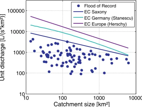
Fig. 2. Comparison of three different envelope curves. The floods of record of Saxon gauges are additionally shown.

Envelope curves are boundary lines above all observed floods of record of a region (see Figs. 2 and 3). Therefore, the floods of recordQFORare normalised by their catchment sizeAand then related toAin a double-logarithmic plot. En-velope curves are determined by their slopeband intercepta (Eq. 1, adapted from Castellarin et al., 2005).

log

QFOR A

= a +b · log(A) (1)

3.1 Empirical envelope curves

In this study, an upper bound with an exceedance proba-bility of zero for Saxony needs to be estimated, since this upper bound discharge is used as an input for a distribution function with upper bound. Three empirical envelope curves were constructed (Fig. 2) and checked for their suitability as upper bound discharge for Saxon gauges. First, an en-velope curve based on the Saxon floods of record only was derived. Second, the envelope curve for Germany ECGfrom Stanescu (2002) was selected. Third, the European envelope curve ECEof Herschy (2002) was used.

The Saxon envelope curve was determined by the largest unit flood of record in Saxony. The floods of record of sev-eral gauges are close to this EC. Thus, it is inconsistent to assume that the Saxon envelope curve has an exceedance probability of zero with respect toTPREC between 150 and 1500 years which were estimated by PRECs for this study region in Guse et al. (2009) (see Sect. 3.4). For a few gaug-ing stations, the discharges provided from PRECs were close to or even larger than the Stanescu envelope curve for Ger-many. Since it was advisable to take an envelope curve which is certain to be the upper bound of Saxon flood discharges, we used the European envelope curve by Herschy (2002). This envelope curve is expected to be an upper bound which might not be exceeded in Saxony, since it is determined by

10 100 1000 10000

1 10 100 1000 10000

Catchment size [km²]

U

n

it

di

s

c

har

ge

[L/(

s

*k

m

²)

]

Regional Envelope Curve

Index Flood (Mean Annual Flood) Regression

Flood of Record

Regional Envelope Curve

Fig. 3. Example of Regional Envelope Curve (REC) (from Guse et al., 2010).

significantly larger floods from the Mediterranean region. Stanescu (2002) and recently Gaume et al. (2009) compared ECs of European countries and determined the largest mag-nitude for Mediterranean countries. Stanescu (2002) con-cluded that larger floods are possible around the Mediter-ranean Sea than in Central European countries, owing to the higher temperature and larger humidity contained in the air masses. The Stanescu envelope curve was used only to in-vestigate the sensitivity of the selection of the empirical en-velope curve (see Sect. 4.3).

3.2 Probabilistic regional envelope curves

For an accurate representation of the upper tail of the dis-tribution function and, in particular, of discharges with re-currence intervals in the order of 1000 years, probabilistic regional envelope curves (PRECs) (Castellarin et al., 2005; Castellarin, 2007) were used. The core idea of the PREC concept is the estimation of an exceedance probability for a regional envelope curve (REC) based on two hypotheses. First, PRECs can be only derived for homogeneous regions as indicated in the index flood method (Dalrymple, 1960; Robson and Reed, 1999). The index flood method assumes regional homogeneity for sites with similar higher moments. We used the mean of the annual maxima series as index flood. The second hypothesis is the scaling of the index flood with the catchment size. The methodical aspects of the PREC concept which are relevant for this study are presented as follows.

the index flood of the given site). Hence, the intercept a is determined by the largest standardised flood of record in the pooling group (Castellarin et al., 2005).

To estimate the recurrence interval of REC, the overall sample years of the annual maxima series (AMS) of all sites of a given homogeneous region are selected. To consider the real information content of the data, the effective sam-ple years of data are calculated. In this way, the reduc-tion of the regional informareduc-tion content of the data due to cross-correlated and concurrent flood sequences is consid-ered. Castellarin (2007) presented an empirical relationship for this case which considers the intersite dependence among the AMS. For a detailed description of this relationship, we refer to Castellarin (2007) and Guse et al. (2009, 2010). The recurrence intervalT of REC is then estimated by using the Hazen plotting position and the number of effective sample years of dataneff(Eq. 2; from Castellarin, 2007)

T = 2 ·neff (2)

The recurrence interval is calculated for the pair of the stan-dardised flood of record and its corresponding catchment size, which governs the REC (Castellarin, 2007). The PREC provides a dischargeQPREC for each gauge of the pooling group with the same recurrence intervalTPREC.

3.3 Application of probabilistic regional envelope curves in Saxony

In previous studies, several PRECs were derived for Sax-ony (Guse et al., 2009, 2010). A major step in the PREC concept is the determination of the pooling group of sites. Guse et al. (2010) used cluster analysis and the Region of Influence (RoI) approach (Burn, 1990) to construct several pooling groups using twenty candidate sets of two or three catchment descriptors and different settings of the two ing methods. An own PREC was constructed for each pool-ing group, which fulfils the homogeneity criteria of the het-erogeneity measure (H1<2) of Hosking and Wallis (1993). Hence, the constitution of the homogeneous regions and thus PRECs differed depending on the grouping procedure.

Guse et al. (2010) estimated the performance of each PREC application by comparing the PREC method with the index flood method. Therefore, the PREC flood quan-tiles were estimated for ungauged conditions using a cross-validation procedure (Castellarin, 2007; Castellarin et al., 2007; Guse et al., 2010). The relative error between PREC discharge and the index flood discharge for the recurrence interval of PREC was calculated (Guse et al., 2010). A high relative error was estimated for sites with a significantly smaller flood of record than theQPRECestimates for this site (see Fig. 7 in Guse et al., 2010). PREC realisations with a low performance error give better additional information than those with a larger one. The flood quantile estimation would not gain by the inclusion of PREC flood quantiles with a high performance error. Hence, PREC flood quantiles with

a relative error<2 were used in this study only. By doing so, PREC realisations that deviated strongly from the index flood method were not considered. This means that PREC flood quantiles of a site, which were more than three times larger for ungauged conditions than the index flood estimates for the sameTPREC, were excluded.

The number of PREC realisations varied among the gauges between 0 and 127. A site had a lower number of PREC flood quantiles when it belonged more often to het-erogeneous regions due to the specific characteristics of this gauge. Of the 89 gauges available in the previous studies, only the 83 gauges with at least one PREC realisation were used for this study (see Fig. 1). In the previous study,TPREC varied between 150 and 1500 years with a mean value of 650 years (Guse et al., 2009).

3.4 Comparison of empirical and probabilistic regional envelope curves

When comparing the traditional empirical envelope curves with the probabilistic regional envelope curves, one has to take note of the differences between the two approaches. In addition to the description of both methods in Sects. 3.1 and 3.2, here we present differences which are relevant for the application in the study region.

Several studies have presented the slope values of empir-ical envelope curves. On average, a slope of−0.5 is esti-mated with values between −0.2 and −0.7 (e.g. Herschy, 2002; Castellarin et al., 2005; Castellarin, 2007; Gaume et al., 2009). In our study, the slopes of the empirical envelope curves are close to−0.4. In contrast, the slope of the PREC realisations in Saxony has a lower negative value in the ma-jority of the cases. Here, the slope b is about−0.2. This means that the effect of the catchment size is smaller.

Since the intercept of the empirical envelope curve is larger than those of the PREC realisations in this study, it follows that the discharge of EC is larger than in the PREC concept. This result is understandable given that we assume in this study that the EC has an exceedance probability of zero, while that of the PREC lies between 6.7×10−4 and 6.7×10−3(the inverse values of 150 and 1500, respectively) for this study region (see Guse et al., 2009).

grouping procedure and as it is shown in Fig. 2 the available number of sites with large catchment sizes was rather low for the PREC applications. It is assumed that the estimation of the empirical envelope curve was better than those of PREC in these cases with a large catchment size. In this way, con-sistency among both methods was ensured.

4 Methods

This study aims at inserting large flood quantiles and up-per bound discharges as additional information into a dis-tribution function to improve the flood quantile estimates for T >100 years. For this purpose, a distribution function is re-quested, into which large flood quantiles derived by PRECs, i.e. QPREC and corresponding TPREC, as well as an upper bound dischargeQMAX, provided by an empirical envelope curve, can be integrated. The method consists of two steps:

1. Integration of the PREC flood quantiles into the ob-served flood series (Sect. 4.1)

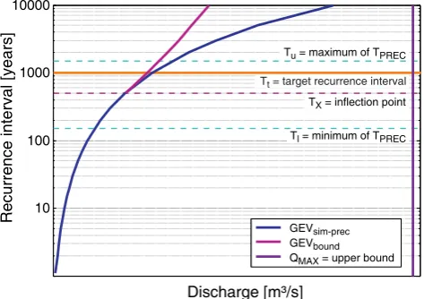
2. Application of a mixed bounded distribution function including PREC flood quantiles and an empirical enve-lope curve discharge as upper bound (Sect. 4.2) Figure 4 gives an overview about our approach, including the most relevant variables. The core idea is an improvement of discharge estimates for a target recurrence intervalTt of 1000 years (orange line in Fig. 4). As additional information, PREC flood quantiles with recurrence intervals between 150 (lower valueTl)and 1500 (upper valueTu) years are used (dashed cyan lines) and combined with the observed flood series in a distribution function (GEVsim−prec). As second additional information, an upper bound discharge (QMAX) (purple line) derived from an empirical envelope curve is in-tegrated into a distribution function. The resulting mixed bounded distribution (GEVbound) consists of two distribu-tion funcdistribu-tions, connected at the inflecdistribu-tion point (TX) (dashed magenta line) and approaching the upper bound (QMAX) asymptotically. The mixed distribution function is identical with GEVsim−precup to the inflection point. From this point on, the bounded GEV is used.

4.1 Integration of PREC flood quantiles

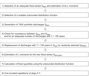
In the first step, PREC flood quantiles were combined with the observed AMS. In a traditional regional flood frequency analysis, flood data from the site itself and from neighbour-ing sites are available. Since a PREC flood quantile com-prises of aQPREC and its correspondingTPREC, it was im-possible to add aQPREC value directly to the AMS as one additional flood value. The additional information of the cor-respondingTPRECneeds to be considered to use the complete information from PRECs. Hence, a novel method was devel-oped. Its steps are illustrated in Fig. 5.

10 100 1000 10000

Discharge [m³/s] GEVsim-prec

QMAX= upper bound

Recurrence interval [years]

GEVbound

T = minimum of Tl PREC T = inflection pointX T = target recurrence intervalt

T = maximum of Tu PREC

Fig. 4. Scheme of the proposed method including the most relevant variable names. The upper bound is illustrated in purple right of the legend. GEV_sim−precis the combined distribution function of the

observed flood series and the PREC flood quantiles. GEVboundis a

bounded distribution function which includes PREC flood quantiles as well as an upper bound discharge.

The Generalised Extreme Value (GEV) distribution was fitted to the observed AMS of each gauge using L-moments (Hosking and Wallis, 1997), denoted as GEVobs. The ade-quacy of the GEV for the flood series in this study was proven by L-moment ratio diagrams (see e.g. Vogel and Fennessey, 1993; Peel et al., 2001).

The three at-site GEVobsparameters (ξ,α,k) were used to generate synthetic flood series. For this,Turandom numbers between 0 and 1 (psim) were generated. Tu was selected, since it was the maximum of TPREC for the study region. Thesepsim values were inserted into the GEV (Eq. 3) re-sulting inTusimulated discharge values, denoted asQ. Q = ξ + α

k ·

h

1 −(−ln(psim))k

i

withk 6= 0 (3) Subsequently, the GEV was fitted toQ, denoted as GEVsim with a new parameter set (ξsim,αsim,ksim).

To ensure consistency between GEVsim and GEVobs, the two should not differ considerably. For this, the flood quan-tiles forT=Tuyears of both GEV functions were compared. It was decided that the discharge estimates of both functions should not vary more than 1% forTu. Otherwise, the random selection ofpsimand the estimation ofQwere repeated.

A second constraint was that there had to be nine or ten values, denoted asnx, larger thanpE=0.9933

=1− 1

150

1) Selection of an adequate flood series Qobsand estimation of its L-moments

2) Selection of a suitable unbounded distribution function

3) Generation of 1500 synthetic discharges Qsim

4) Check for consistency between Q and Q

and for an adequate number of discharges with T > 150 yearssim obs

5) Replacement of discharges with T > 150 years in Qsimby randomly selected QPREC

6) Estimation of L-moments for the new flood series Q_sim-prec

7) Calculation of flood quantiles using the unbounded distribution function

8) One hundred repetitions of steps 5-7

Fig. 5. Overview of the consecutive steps to integrate PREC flood quantiles into the at-site distribution function.

selected number of PREC flood quantiles. Then, GEVsimand GEVobswere assumed as sufficiently similar for using theTu simulated flood series instead of the shorter measured time series.

In a next step, PREC flood quantiles were integrated into the simulated flood seriesQsim. Among the random num-berspsim, thenx values larger thanpE were removed from the simulated flood seriesQsim and replaced by nx QPREC values. This approach implicitly assumes that the observed flood series is appropriate up toTl. However, the PREC dis-charges also influenced the combined function of observed and PREC discharges forT < Tl.

Since previous studies provided more thannxPREC flood

quantiles for most of the gauges (see Sect. 3.3) (Guse et al., 2010), nx PREC flood quantiles among the PREC

re-alisations of a given gauge were selected in a random pro-cess whereas the discharges were weighted according to their TPREC. We considered the recurrence intervals using a bino-mial functionB(Eq. 4). This approach was used to estimate the mean occurrence of a specificQPRECwith a recurrence intervalTPRECwithinTuyears.

P (X=m) = B_T

u; _T 1

PREC

(X=m)withm= 1,2,...,20 (4) We checked m for one to twenty occurrences. Among these twenty results, we selected the m with the largest probability Pmax, i.e. the maximum likelihood, denoted as mmax. The QPREC value of this PREC realisation was assigned mmax

times to a vectorVPREC. This implies that PREC discharges with a smallerT were assigned more often to VPREC. In this way, the recurrence interval of the PREC realisations was evidently considered, since a PREC flood quantile with a smallerTPREC was expected to occur more often than a PREC flood quantile with a larger one. This procedure was repeated for all PREC realisations of this gauge.

Thenx QPREC values were then randomly selected

with-out replacement fromVPREC. In order to adequately repre-sentTPREC, a specificQPRECcould be selected as many times as it was included inVPREC. Thenxdischarges derived from

PREC were assigned to the reduced simulated flood series ofTu−nxvalues, so that the new flood series comprisedTu values again.

In the majority of cases, the length ofVPREC was larger thannx, which required the random selection of PREC

dis-charges. In the other cases, for sites with a lower number of PREC realisations inVPRECthannx,nx values were

re-moved from the simulated flood series as well. Then all val-ues from VPREC were added. In order to obtain Tu values again, the remaining discharges toTuwere selected randomly from thenxdischarges withT > Tlyears.

and therefore also in the final distribution function. Hence, we repeated the selection ofQPREC one hundred times and estimated one hundred GEV parameter sets. The GEV parameter sets which estimated the median discharge for Tt=1000 years were used for the next steps. The corre-sponding GEV distribution was denoted as GEVsim−prec 50. The influence of the PREC selection on the discharge esti-mates was expressed by showing the 5%- and 95%-quantiles of GEVsim−prec for Tt, denoted as GEVsim−prec 05 and GEVsim−prec 95, respectively. A comparison of GEVsim−prec with GEVsimillustrated the effect of using PREC flood quan-tiles as additional information.

4.2 Mixed bounded distribution function

We used a mixed bounded distribution function which was developed in storm research (Hofherr et al., 2008). The use of this distribution function enables us to integrate an upper bound discharge as further additional information besides of the PREC flood quantiles.

In this mixed bounded distribution function, flood quan-tiles up to a recurrence interval threshold ofTX (inflection point) are estimated by an unbounded distribution function (here: GEVsim−precwithk <0), and quantiles above the in-flection point TX are estimated by a bounded distribution (here: GEVbound). GEVsim−prec includes PREC discharges which are representative forT between 150 and 1500 years. To adequately represent the PREC discharges, we selected an inflection point TX=500 years. The sensitivity of the method to the choice of this inflection point was analysed in Sect. 4.3.

GEVbound has a positive shape parameter k and, hence, asymptotically approaches an upper bound. The three param-eters of GEVbound (ξbound,αbound,kbound) were determined with a numerical solution method by three constraints using Eqs. (5)–(7). First, the upper boundQMAXwhich was pro-vided by an empirical envelope curve was inserted into the GEV upper bound function (Eq. 5).

QMAX = ξbound + αbound

kbound (5)

Second, both GEV functions (GEVsim−prec, GEVbound) had to be identical at the inflection point to avoid inconsistencies. Therefore, both functions were equated at the inflection point (Eq. 6).

GEVsim−prec(T = Tx) = GEVbound(T = Tx) (6)

The third constraint was that both GEV functions had the same slope at the inflection point. Therefore, their derivates were equated (Eq. 7).

GEVsim−prec0(T = Tx) = GEVbound0(T =Tx) (7)

In the case of a successful solution, GEVboundwas fully de-fined, increasing monotonically.

The mixed bounded distribution function was not applied for the seven sites with a positivekof GEVsim−prec. In these cases, the GEVsim−precwas already bounded. Since they al-ready approach an upper bound, even after integrating PREC discharges, the number of sites for which the mixed bounded distribution function was applied was reduced to 76. The main advantage of a bounded distribution function is that it avoids an unlimited increase up to unrealistic discharge val-ues, which was already prevented by the positivekvalues in these cases. In this context, it is worth mentioning that ten sites have a positivekfor the at-site estimation. This means that the sign has been changed from positive to negative for three sites due to the inclusion of the PREC flood quantiles. 4.3 Sensitivity analysis

The effect of three choices in this method was investigated for a target recurrence intervalTt=1000 years in a combined sensitivity analysis. The sensitivity of each choice was tested as follows:

1. The magnitude of the empirical envelope curve dis-charge: German EC (ECG) (Stanescu, 2002) vs. Eu-ropean EC (ECE) (Herschy, 2002),

2. the selection of PREC discharges: 5% vs. 95% of the GEVsim−precestimates forTt,

3. and the magnitude of the recurrence interval threshold (inflection point):TX=200 vs. 500 years.

For each choice, the four possible combinations of the two other choices were checked. The comparison ofQbound (Tt=1000)between all possible combinations of these three choices allowed us to evaluate their effect on the discharge estimations of GEVbound forTt. The relative deviations are calculated for each choice (Eqs. 8–10). This procedure en-abled us to determine the most sensitive choice of the dis-charge estimates forTt.

EEC =

Qbound(QMAX = ECE) −Qbound(QMAX = ECG) Qbound(QMAX = ECG) (8) EPREC =

Qbound GEVsim−prec,95−Qbound GEVsim−prec,5

Qbound GEVsim−prec,5

(9)

ETX =

Qbound (TX = 500) −Qbound(TX = 200)

Qbound(TX = 200) (10)

5 Results

5.1 Integration of PREC flood quantiles

0 50 100 150 200 10

100 1000 10000

Lauenstein

Discharge [m³/s]

PLP Hazen GEV_obs GEVsim

GEV_{sim-prec 50} PREC results (all) PREC results (selected)

Recurrence interval [years]

Fig. 6. Effect of integrating PREC flood quantiles into the at-site flood frequency analysis. GEVobs, GEVsim and GEVsim−precare

compared for the site Lauenstein. The observed flood series is il-lustrated as Hazen plotting position (PLP Hazen). The PREC flood quantiles which were selected for GEVsim−prec 50are coloured in

blue.

for GEVsim−prec 50. Most of theQPREC(TPREC) are smaller than theQGEV(TPREC). Hence, the integration of the PREC flood quantiles leads to a higherk(shape parameter of GEV) and a lower skewness of GEVsim−preccompared to GEVsim. Therefore,Qsim−precfor a givenT is smaller thanQsim.

The PREC flood quantiles indicate that the skewness of the GEV might be too large when using the observed data only. The recurrence interval of the flood of record (flood discharge of 2002) might be larger than the at-site estimate. The effect of the flood of record on the estimation of large quantiles within the at-site flood frequency analysis seems to be too high. The smallest PREC discharge is identical with the flood of record of Lauenstein. This means that the intercept of this REC was determined by the at-site flood of record.

5.2 Mixed bounded distribution function

GEVsim−prec was used to estimate the flood quantiles up to TX=500 years in the mixed bounded distribution ap-proach. FromTXon, GEVboundwas used, which asymptoti-cally approaches the upper bound discharge derived from the empirical envelope curve by Herschy (2002). Considering GEVobsand GEVboundfor all gauges, three cases can be dis-tinguished, which are shown in Fig. 7a–c. The variability due to the selection of PREC flood quantiles is demonstrated by adding the 5%- and 95%-quantiles (cyan dashed line).

In the first case (gauge Lauenstein, Fig. 7a), GEVbound es-timates lower discharges than GEVobs for all values of T. To give an example, GEVbound estimates a discharge of 200 m3/s for Tt, whereas the GEVobs discharge is about

0 200 400 600 800 1000

10 100 1000

10000 Lauenstein

Discharge [m³/s]

R

e

c

u

rr

enc

e

int

er

v

a

l

[y

ear

s

]

PLP Hazen GEVobs GEV_sim-prec GEV_{sim-prec 05 and 95} PREC results (all) PREC results (selected) GEVbound 50 GEV_{bound 05 and 95} Upper bound

0 500 1000 1500 2000 2500 3000 3500 4000 10

100 1000 10000

Niederschlema

Discharge [m³/s]

R

e

c

u

rr

enc

e

int

er

v

a

l

[y

ear

s

]

PLP Hazen GEV_obs GEV_sim-prec GEVsim-prec 05 and 95 PREC results (all) PREC results (selected) GEV_{bound 50} GEV_{bound 05 and 95} Upper bound

0 1000 2000 3000 4000 5000 6000 10

100 1000

10000 Gera

Discharge [m³/s]

R

e

c

u

rr

enc

e

int

er

v

a

l

[y

ear

s

]

PLP Hazen GEV_obs GEVsim-prec GEVsim-prec 05 and 95 PREC results (all) PREC results (selected) GEV_{bound 50} GEVbound 05 and 95 Upper bound a)

b)

c)

Fig. 7. The mixed bounded distribution function GEVboundvs. the

traditional GEV (GEV_obs) and the GEV_sim−prec for the gauges

(a) Lauenstein, (b) Niederschlema, (c) Gera. The blue-coloured PREC results show the selected PREC discharges which yielded a median discharge for the target recurrence interval of 1000 years among the hundred repetitions. The upper bound is illustrated in purple right of the legend.

300 m3/s. GEVobsincreases unlimitedly, whereas the gradi-ent of GEVbounddecreases and approaches the upper bound. Figure 7b shows an example (gauge Niederschlema, site 33 in Fig. 1) where several PREC discharges are larger than the GEVobsdischarge estimates for the same recurrence interval. However, there are also various smaller PREC flood quantiles. On average,QPREC (TPREC)is similar to QGEV (TPREC), and therefore Qsim−prec is similar to Qobs. The PREC flood quantiles support the GEVobs estimations, and the effect of the inclusion of PREC discharges is low.

0 10 20 30 40 50 60 70 80 -0.6

-0.4 -0.2 0 0.2 0.4 0.6 0.8 1

Site

R

e

l.

dev

ia

ti

on

Lauenstein

Niederschlema Gera

Fig. 8. Comparison of discharges estimated by GEVsim and

GEVsim−prec 50for the target recurrence interval of 1000 years for

83 gauges. The three sites shown in Fig. 7 are marked.

discharges. The PREC flood quantiles indicate that a flood larger than the current flood of record might occur. The ma-jority of the sites belongs to this third type.

5.3 Comparison of the three distribution functions

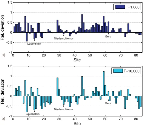
First, we compared GEVsimand GEVsim−prec. After that, we examined the differences between GEVsimand GEVbound. In both cases, discharge estimates forTtwere compared by cal-culating the relative deviations and we used the median of the hundred GEV estimations for GEVsim−precand GEVbound.

The comparison of GEVsim and GEVsim−prec 50 shows how strongly GEVsim−prec 50 is affected by PREC flood quantiles. Figure 8 illustrates that the relative deviation is positive in the majority of the cases. Hence, GEVsim−prec 50 estimates larger discharges than GEVsim for almost all gauges. This result can be explained by the PREC flood quantiles. For the majority of the sites, theQPREC (TPREC) values are larger than the correspondingQGEV (TPREC) es-timates. Hence, GEVsim−prec 50also estimates larger values than GEVsim(see “Gera” type in Fig. 7c).

In a further step,QsimandQbound 50are compared (Fig. 9). A positive relative deviation indicates thatQbound 50is larger thanQsimdespite the asymptotic behaviour towards the up-per bound. The Qbound 50 exceeds Qsim, because QPREC (TPREC)values are mostly larger in comparison to the corre-spondingQGEV(TPREC)(see example of Gera; Fig. 7c). This implies that the PREC discharges enormously affect the GEV and lead to larger discharges of GEVbound 50 than GEVsim for the same recurrence interval. Figure 9b shows that even forT= 10 000 years a positive relative deviation is estimated for the half of the sites. Due to the asymptotic behaviour of GEVbound 50, there are more sites with a negative relative deviation forT= 10 000 than forT =1000 years.

5.4 Sensitivity analysis

With a combined sensitivity analysis, the effect of the up-per bound derived by the empirical envelope curve, of the QPREC-selection and of the inflection point is investigated.

0 10 20 30 40 50 60 70 80

-1 -0.5 0 0.5 1 1.5

Site

Rel.

deviation

T=10,000

Gera

Niederschlema Lauenstein

b)

0 10 20 30 40 50 60 70 80

-1 -0.5 0 0.5 1 1.5

Site

Rel.

deviation

T=1,000

Lauenstein

Niederschlema Gera

a)

Fig. 9. Comparison of discharges estimated by GEVsim

and GEVbound 50 for recurrence intervals of (a) 1000 and

(b) 10 000 years. The three sites shown in Fig. 7 are marked. The seven sites with a positivekare not shown.

Each sub-figure in Fig. 10 illustrates the results of one choice. The four possible combinations of the two other choices (see Sect. 4.3) are shown with four box-plots. Each box-plot is based on the results of the 76 sites. Figure 10a–c illus-trate that the largest relative deviation is found when com-paring the 5%- and 95%-quantiles of GEVsim−precand em-phasise that it is necessary to consider different PREC selec-tions. This variation occurs due to the random selection of the PREC discharges.

The selection of the empirical envelope curve has the lowest relative deviation. There are only small differ-ences in Fig. 10a. Its effect is slightly larger for TX=

200 years. The smallerTX, the smaller is the point at which GEVboundasymptotically approaches to the upper bound and the stronger GEVbound is influenced by the empirical enve-lope curve discharge.

The relative deviation due to the PREC selection is similar when varying the empirical envelope curve or the inflection point (Fig. 10b). Here, there is the inverse situation com-pared to the selection of the empirical envelope curve. The largest relative deviation is found forTX=500 years. This can be explained by the fact that, GEVboundis affected from TXon also by the asymptotic behaviour and not only by the selection ofQPREC.

c) b) a)

ECGT 200X EC T 200E X ECGT 500X EC T 500E X

0 0.1 0.2 0.3 0.4 0.5

0.6 PREC-95 vs. PREC-05

Re

l.

d

e

v

ia

ti

o

n

PREC 95 T 200X PREC 05 T 200X PREC 95 T 500X PREC 05 T 500X

0 0.1 0.2 0.3 0.4 0.5

0.6 EC Germany (Stanescu) vs. EC Europe (Herschy)

Re

l.

d

e

v

ia

ti

o

n

ECGPREC 95 ECGPREC 05 EC PREC 95E EC PREC 05E

0 0.1 0.2 0.3 0.4 0.5

0.6 T = 200 vs. T = 500 yearsX X

Re

l.

d

e

v

ia

ti

o

n

Fig. 10. Relative deviation between the quantile estimates of GEVbound forT=1000 years when varying three choices. The

boxplots show the results for the 76 sites which were used in the sensitivity analysis.

(a) Empirical envelope curves (EC_G= Germany; Stanescu, 2002; ECE= Europe; Herschy, 2002), (b) PREC flood discharges (9,

5-quantiles) and (c) inflection point (TX).

The relative importance of the three choices is shown for all 76 gauges (Fig. 11). For each choice, the mean of the absolute relative deviation of the four approaches as indi-cated in Fig. 10 was estimated for each site separately. In a next step, the three mean absolute relative deviations were summed up (overall absolute relative deviation) and the frac-tions of the three choices were estimated. In this way, the importance of the three choices for all sites is given. The gauges are ordered by the distance between their unit floods of record andEEC. Figure 11 shows that the effect of the selection of the PREC flood discharges increases with larger distance to the REC, whereas the effect of the inflection point and of the empirical envelope curve decreases. This pattern can be explained when considering the three choices in de-tail.

0 10 20 30 40 50 60 70

0 0.2 0.4 0.6 0.8 1

Site

Fr

ac

ti

on

of

th

e

c

hoi

c

es

EC PREC TX

Fig. 11. Fraction of the three choices to the overall absolute relative deviation for each site in [%]. The sites are ordered by the distance of the unit flood of record to the unit discharge of the European en-velope curve.

EC = selection of the empirical envelope curve (EC_G vs. EC_E); PREC = selection of PREC flood discharges (95- vs. 5-quantiles);

TX= selection of the inflection point (TX=200 vs. 500 years).

The effect of the choice of the empirical envelope curve considerably influences the discharge estimates forTt only for sites with a small distance to the largest unit flood of record, i.e. the sites which are close to the empirical envelope curve. The closer they are to the European one, the larger is the fraction of the empirical envelope curve selection.

The intercept of a REC is defined by the largest standard-ised flood of record in the pooling group. The site which determines in all its PREC realisations the intercept of REC (Neundorf, site 9 in Fig. 1) has a relative deviation of zero related to theQPREC selection (site 3 in Fig. 11), because QPREC is always equal to the at-site flood of record. The smaller the at-site unit flood of record, the larger the distance to the largest unit flood of record of a pooling group could be within a REC. Because of that, the possible range of PREC discharges increases along with the distance between the at-site unit flood of record and the largest regional unit flood of record.

In addition, the effect ofTXis larger for sites with a high skewness. The larger the skewness, the larger are the differ-ences between the discharge estimates forT =200 vs.T =

500 years. Therefore, the influence of the choice ofTXalso increases. Especially the sites with a large flood of record are characterised by a high skewness. Thus, the largest influence of theTX selection is found for sites with floods of record close to EC. The fraction of the inflection point is highly correlated with the shape parameterk. The effect of the in-flection point is negligible for sites with a small negativek, whereas its effect predominates whenkis highly negative.

6 Discussion

bound discharge. It is interesting to compare this method with the integration of historical events, to discuss the selec-tion of PREC flood quantiles and the results of the sensitivity analysis and to compare our procedure with traditional flood regionalisation methods.

There are some similarities between our method to inte-grate PREC flood quantiles and the use of historical floods as additional information in flood frequency studies. Historical floods are combined as non-systematic data with measured flood series. Generally, a threshold is fixed and the number of floods above this threshold in the historical period is de-termined (Stedinger and Cohn, 1986; Reis Jr. and Stedinger, 2005). The integration of historical information is based on the assumption that all extreme floods above the threshold are recorded because of the large amount of damages they have caused. However, in this approach discharge values are used only. The probabilities of the historic floods are un-known and are not considered (e.g. Martins and Stedinger, 2001). This is the largest difference to our method, which considers besides the discharge values also the recurrence in-terval of PRECs. Furthermore, whereas the use of historical data extends the time series, the integration of PREC flood quantiles is based on substituting the time period with spatial information. Because of that, a different approach than for the integration of historic data was chosen, which enabled us to use the additional information in terms ofTPREC and to integrate severalQPRECvalues.

The selection of the PREC flood quantiles is the most sensitive step forTt. The influence of the random process depends on two aspects. First, it is affected by the num-ber of PREC realisations. The more PREC realisations, the more combinations of randomly selected PREC discharges are possible. Second, the results are influenced by the vari-ation of the PREC flood quantiles inQPRECas well as in its correspondingTPREC. Small differences between the PREC flood quantiles lead to low differences in GEVsim−prec inde-pendently of the number of PREC realisations.

The selection of the inflection point has the second largest effect. The inflection points were selected according to the aim of our study and the available data and PREC results. Based on the observed data, flood quantiles up to about 100 years can be estimated by at-site analysis. The recur-rence interval of interest was 1000 years. Hence, we checked intermediate recurrence intervals as inflection point (200 and 500 years) to quantify the sensitivity of this choice. We fi-nally selected an inflection point of 500 years, because the higher inflection point leads to a better consideration of the PREC flood quantiles. The larger the inflection point, the larger is the effect of the PREC flood quantiles.

As illustrated in Fig. 2, both empirical envelope curves dif-fer strongly. However, the sensitivity analysis shows that the effect of the envelope curve selection on a discharge with T=1000 years is smaller than those of the random selection of PREC discharges or of the inflection point. In this con-text, it is worth noting that we predefined a target recurrence

interval of 1000 years. Since the envelope curve governs the asymptotical approach towards the upper bound, the influ-ence of the envelope curve selection will be larger for in-creasingT.

In traditional flood regionalisation approaches (e.g. index flood), the recurrence interval of interests can be increased successively by the inclusion of neighbouring data. Or, in other words, the uncertainty of large flood quantiles de-creases with each added flood series that leads to a gain of information, and consequently, to an increase of the effec-tive observation data. Our procedure differs from traditional methods, because it is based on two types of additional infor-mation (PREC flood quantiles and upper bound discharge) which are representative for specific parts of the distribu-tion funcdistribu-tion. The target recurrence interval of 1000 years is covered by the PREC flood quantiles adequately. It is clear that we did not consider additional information to the at-site flood data for recurrence intervals smaller than the PREC flood quantiles (150 years). However, also the estimation of discharges with recurrence intervals smaller than 150 years might benefit from the use of PREC flood quantiles as addi-tional information. A combination of our procedure with a traditional regionalisation approach could be a next step to increase the use of additional information.

7 Conclusions

A novel method to improve the quantile estimation for high recurrence intervals by using additional information was pre-sented. Our study was focused on a recurrence interval of 1000 years. Large flood quantiles were derived by proba-bilistic regional envelope curves (PREC). These PREC flood quantiles were combined with the measured flood series. A mixed bounded distribution function was presented which considers in addition to the PREC flood quantiles also an up-per bound discharge derived by an empirical envelope curve. The mixed bounded distribution function avoids an increase up to unrealistic large discharges. Whereas the combination of PREC discharges and a simulated flood series based on at-site parameters was used for recurrence intervals of up to 500 years, a bounded distribution function was applied for largerT.

The main outcomes of this study are:

1. The use of the additional information of PREC flood quantiles and empirical envelope curves supports the es-timation of large quantiles.

2. The effect of PREC flood quantiles on the quantile esti-mation is especially relevant when the PREC discharge varies largely from the at-site GEV estimate for the same recurrence interval.

upper bound discharge on a flood quantile of 1000 years is smaller than the selection of PREC flood quantiles and of the inflection point between both functions of the mixed bounded distribution.

Acknowledgements. This work is part of the Center for

Disas-ter Management and Risk Reduction Technology (CEDIM) (http: //www.cedim.de), a joint venture between the Helmholtz Centre Potsdam – GFZ German Research Centre for Geosciences and the Karlsruhe Institute of Technology (KIT). We thank CEDIM and the GFZ for the financial support.

We thank the State Agency of Environment and Geology of the Free State of Saxony for the permission to use the

dis-charge data. Furthermore we thank the State Agency for

En-vironment of Thuringia for additional discharge data. We also

thank the Federal Agency for Cartography and Geodesy of Ger-many (BKG) for the ATKIS-Basis-DLM and the digital elevation model for Saxony (BKG GeoDataCentre, 2005). The SRTM Dig-ital Terrain Model was downloaded from (http://srtm.csi.cgiar.org/ SELECTION/inputCoord.asp, 19 May 2008) (Jarvis et al., 2008).

We gratefully acknowledge the very helpful advices from an anonymous referee and Attilio Castellarin in HESSD.

Edited by: H. Madsen

References

Benito, G., Lang, M., Barriendos, M., Llasat, M. C., Franc´es, F., Ouarda, T. B. M. J., Thorndycraft, V. R., Enzel, Y., B´ardossy, A., Coeur, D., and Bob´ee, B.: Use of Systematic, Palaeoflood and Historical Data for the Improvement of Flood Risk Estima-tion, Review of Scientific Methods, Nat. Hazards, 31(3), 623– 643, 2004.

BKG GeoDataCentre (Federal Agency for Cartography and Geodesy): Digital Landscape Model ATKIS Basis DLM, Frank-furt/Main, 2005.

Burn, D. H.: Evaluation of Regional Flood Frequency Analysis with a Region of Influence Approach, Water Resour. Res., 26(8), 2257–2265, 1990.

Castellarin, A.: Probabilistic envelope curves for design flood es-timation at ungauged sites, Water Resour. Res., 43(4), W04406, doi:04410.01029/02005WR004384, 2007.

Castellarin, A., Vogel, R. M., and Matalas, N. C.: Probabilistic be-haviour of a regional envelope curve, Water Resour. Res., 41, W06018, doi:06010.01029/02004WR003042, 2005.

Castellarin, A., Vogel, R. M., and Matalas, N. C.: Multivariate prob-abilistic regional envelopes of extreme floods, J. Hydrol., 336(3– 4), 376–390, 2007.

Chbab, E. H., Buiteveld, H., and Diermanse, F.: Estimating ex-ceedance frequencies of extreme river discharges using statisti-cal methods and physistatisti-cally based approach, ¨Osterr. Wasser- und Abfallwirtschaft, 58(3–4), 35–43, 2006.

Cohn, T. A. and Stedinger, J. R.: Use of Historical Information in a Maximum Likelihood Framework, J. Hydrol., 96(1–4), 215–233, 1987.

Condie, R. and Lee, K. A.: Flood frequency analysis with historic information, J. Hydrol., 58(1–2), 47–61, 1982.

Costa, J. E.: A comparison of the largest rainfall-runoff floods in the United States with those of the People’s Republic of China and the world, J. Hydrol., 96(1–4), 101–115, 1987.

Crippen, J. R.: Envelopes Curves for Extreme Flood Events, J. Hy-draul. Eng.-ASCE, 108(8), 1208–1212, 1982.

Dalrymple, T.: Flood frequency analyses, US Geol. Surv. Water Supply Pap., 1543-A, 1960.

El Adlouni, S., Bob´ee, B., and Ouarda, T. B. M. J.: On the tails of extreme event distributions in hydrology, J. Hydrol., 355(1–4), 16–33, 2008.

England Jr., J. F., Jarrett, R. D., and Salas, J. D.: Data-based com-parisons of moments estimators using historical and paleoflood data, J. Hydrol., 278(1–4), 172–196, 2003a.

England Jr., J. F., Salas, J. D., and Jarrett, R. D.: Comparisons of two moments-based estimators that utilize historical and pale-oflood data for the log Pearson type III distribution, Water Re-sour. Res., 39(7), 1243, doi:1210.1029/2002WR001791, 2003b. Enzel, Y., Ely, L. L., House, P. K., Baker, V. R., and Webb, R. H.:

Paleoflood evidence for a natural upper bound to flood magni-tudes in the Colorado River basin, Water Resour. Res., 29(5), 2287–2298, 1993.

Fernandes, W. and Naghettini, M.: Integrated frequency analysis of extreme flood peaks and flood volumes using the regional-ized quantiles of rainfall depths as auxiliary variables, J. Hydrol. Eng.-ASCE, 13(3), 171–179, 2008.

Fernandes, W., Naghettini, M., and Loschi, R.: A Bayesian ap-proach for estimating extreme flood probabilities with upper-bounded distribution functions, Stoch. Env. Res. Risk A., 24(8), 1127–1143, doi:10.1007/s00477-010-0365-4, 2010.

Franc´es, F.: Using the TCEV distribution function with systematic and non-systematic data in a regional flood frequency analysis, Stoch. Hydrol. Hydraul., 12(4), 267–283, 1998.

Franc´es, F. and Botero, B. A.: Probable maximum flood estima-tion using systematic and non-systematic informaestima-tion, in: Pale-ofloods, Historical Floods and Climatic Variability: Applications in Flood Risk Assessment, Proceedings of the PHEFRA work-shop, edited by: Thorndycraft, V. R., Benito, G., Barriendos, M., and Llasat, M. C., Barcelona/Spain, 223–229, 2003.

Gaume, E., Bain, V., Bernardara, P., Newinger, O., Barbuc, M., Bateman, A., Blaskovicova, L., Bl¨oschl, G., Borga, M., Dumitrescu, A., Daliakopoulos, I., Garcia, J., Irimescu, A., Kohnov´a, S., Koutroulis, A., Marchi, L., Matreata, S., Medina, V., Precisco, E., Sempere-Torres, D., Stancalie, G., Szolgay, J., Tsanis, I., Velasco, D., and Viglione, A.: A compilation of data on European flash floods, J. Hydrol., 367(1–2), 70–78, 2009. Guillot, P. and Duband, D.: La m´ethode du gradex pour le

cal-cul de la probabilit´e des crues `a partir des pluies, Floods and Their Computation – Proceedings of the Leningrad Symposium, IAHS-AISH P., 84, 560–569, 1967.

Guse, B., Castellarin, A., Thieken, A. H., and Merz, B.: Effects of intersite dependence of nested catchment structures on prob-abilistic regional envelope curves, Hydrol. Earth Syst. Sci., 13, 1699–1712, doi:10.5194/hess-13-1699-2009, 2009.

Gutknecht, D., Bl¨oschl, G., Reszler, C., and Heindl, H.: A “Multi-Pillar”-Approach to the Estimation of Low Probability Design Floods, ¨Osterr. Wasser- und Abfallwirtschaft, 58(3–4), 44–50, 2006.

Herschy, R.: The world’s maximum observed floods, Flow Meas. Instrum., 13, 231–235, 2002.

Hofherr, T., Kottmeier, C., Heneka, P., and Ruck, B.: Wintersturm Risiko Modell und Echtzeit-Schadensprognose, in: CEDIM En-twicklungsbericht Dezember 2008, edited by: CEDIM – Center for Disaster Management and Risk Reduction Technology, un-published work, 17–19, 2008.

Hosking, J. R. M. and Wallis, J. R.: Paleoflood hydrology and flood frequency analysis, Water Resour. Res., 22(4), 543–550, 1986a. Hosking, J. R. M. and Wallis, J. R.: The value of historical data in

flood frequency analysis, Water Resour. Res., 22(4), 1606–1612, 1986b.

Hosking, J. R. M. and Wallis, J. R.: Some statistics useful in re-gional frequency analysis, J. Hydrol., 29(2), 271–281, 1993. Hosking, J. R. M. and Wallis, J. R.: Regional frequency analysis:

an approach based on L-moments, Cambridge University Press, Cambridge, UK, 1997.

Houghton-Carr, H.: Flood Estimation Handbook 4:

Restate-ment and application of the Flood Studies Report rainfall-runoff method, Institute of Hydrology, Wallingford, UK, 1999. Jarvis, A., Reuter, H. I., Nelson, A., and Guevara, E.: Hole-filled

SRTM for the globe Version 4, available from the CGIAR-CSI SRTM 90 m Database, http://srtm.csi.cgiar.org, last access: 19 May, 2008.

Kanda, J. A.: A New Extreme Value Distribution With Lower and Upper Limits For Earthquake Motion and Wind Speeds, Theor. Appl., 31, 351–360, 1981.

Martins, E. S. and Stedinger, J. R.: Historical information in a gen-eralized maximum likelihood framework with partial duration and annual maximum series, Water Resour. Res., 37(8), 2559– 2567, 2001.

Merz, R. and Bl¨oschl, G.: Flood frequency hydrology: 1. Temporal, spatial, and causal expansion of information, Water Resour. Res., 44, W08432, doi:08410.01029/02007WR006744, 2008a. Merz, R. and Bl¨oschl, G.: Flood frequency hydrology: 2.

Com-bining data evidence, Water Resour. Res., 44, W08433, doi:08410.01029/02007WR006745, 2008b.

Merz, B. and Thieken, A. H.: Separating Natural and Epistemic Uncertainty in Flood Frequency Analysis, J. Hydrol., 309(1–4), 114–132, 2005.

Merz, B. and Thieken, A. H.: Flood risk curves and uncertainty bounds, Nat. Hazards, 51(3), 437–458, 2009.

Merz, R., Bl¨oschl, G., and Humer, G.: National flood discharge mapping in Austria, Nat. Hazards, 46(1), 53–72, 2008.

Moon, Y.-I., Lall, U., and Boswarth, K.: A comparison of tail prob-ability estimators for flood frequency analysis, J. Hydrol., 151(2– 4), 343–363, 1993.

Naghettini, M., Potter, K. W., and Illangasekare, T.: Estimating the Upper Tail of Flood-Peak Frequency Distributions Using Hydrometeorological Information, Water Resour. Res., 32(4), 1729–1740, 1996.

Peel, M. C., Wang, Q. J., Vogel, R. M., and McMahon, T. A.: The Utility of L-moment ratio Diagrams for selecting a regional prob-ability distribution, Hydrolog. Sci. J., 46(1), 147–156, 2001. Petrow, Th., Thieken, A. H., Kreibich, H., Bahlburg, C. H.,

and Merz, B.: Improvements on flood alleviation in Germany: Lessons learned from the Elbe flood in August 2002, Environ. Manage., 38(3), 717–732, 2006.

Petrow, Th., Merz, B., Lindenschmidt, K.-E., and Thieken, A. H.: Aspects of seasonality and flood generating circulation pat-terns in a mountainous catchment in south-eastern Germany, Hy-drol. Earth Syst. Sci., 11, 1455–1468, doi:10.5194/hess-11-1455-2007, 2007.

Pohl, R.: Historische Hochwasser aus dem Erzgebirge, Fakult¨at Bauingenieurwesen, Institut f¨ur Wasserbau und Technische Hy-dromechanik, Technische Universit¨at Dresden, Dresden Wasser-bauliche Mitteilungen, Heft 28, 2004.

Reis Jr., D. S. and Stedinger, J. R.: Bayesian MCMC flood fre-quency analysis with historical information, J. Hydrol., 313(1– 2), 97–116, 2005.

Robson, A. and Reed, D.: Flood Estimation Handbook 3: Statistical procedures of flood frequency estimation, Institute of Hydrology, Wallingford, UK, 338 pp., 1999.

Rossi, F., Fiorentino, M., and Versace, P.: Two component extreme value distribution for flood frequency analysis, Water Resour. Res., 20(5), 847–856, 1984.

Schumann, A. H.: Das hydrologische Risiko bei der

Bemes-sung und der Bewirtschaftungsplanung von Talsperren, Wasser-bauliche Mitteilungen, Heft 27, 33–46, 2004.

Schumann, A. H.: Flood statistical assessment of the event from August 2002 in the Mulde river basin, based on seasonal statis-tics, in German: Hochwasserstatistische Bewertung des Au-gusthochwassers 2002 im Einzugsgebiet der Mulde unter An-wendung der saisonalen Statistik, Hydrol. Wasserbewirts., 49, 200–206, 2005.

Stanescu, V. A.: Outstanding floods in Europe, A regionalization and comparison, International Conference on Flood Estimation, Berne, Switzerland, 697–706, 2002.

Stedinger, J. R. and Cohn, T. A.: Flood frequency analysis with historical and paleoflood information, Water Resour. Res., 22(3), 785–793, 1986.

Stedinger, J. R., Vogel, R. M., and Foufoula-Georgiou, E.: Fre-quency Analysis of extreme events, in: Handbook of Hydrology, edited by: Maidment, D. A., McGraw-Hill, New York, 18.11– 18.66, 1993.

Thieken, A. H., M¨uller, M., Kreibich, H., and Merz, B.: Flood damage and influencing factors: New insights from the Au-gust 2002 flood in Germany, Water Resour. Res., 41(12), W12430, doi:101029/102005WR004177, 2005.

Ulbrich, U., Br¨ucher, T., Fink, A. H., Leckebusch, G. C., Kr¨uger, A., and Pinto, J. G.: The central European floods of August 2002: part 1 – Rainfall periods and flood development, Weather, 58(8), 371–377, 2003.