Open Access
Methodology article
Improved ChIP-chip analysis by a mixture model approach
Wei Sun*
1, Michael J Buck
2, Mukund Patel
3and Ian J Davis*
3,4Address: 1Department of Biostatistics, Carolina Center for Genome Sciences, University of North Carolina at Chapel Hill, Chapel Hill, NC, USA, 2Department of Biochemistry, Center of Excellence in Bioinformatics and Life Sciences, State University of New York at Buffalo, Buffalo, NY, USA, 3Department of Genetics, University of North Carolina at Chapel Hill, Chapel Hill, NC, USA and 4Department of Pediatrics, Lineberger
Comprehensive Cancer Center, University of North Carolina at Chapel Hill, Chapel Hill, NC, USA
Email: Wei Sun* - [email protected]; Michael J Buck - [email protected]; Mukund Patel - [email protected]; Ian J Davis* - [email protected]
* Corresponding authors
Abstract
Background: Microarray analysis of immunoprecipitated chromatin (ChIP-chip) has evolved from
a novel technique to a standard approach for the systematic study of protein-DNA interactions. In ChIP-chip, sites of protein-DNA interactions are identified by signals from the hybridization of selected DNA to tiled oligomers and are graphically represented as peaks. Most existing methods were designed for the identification of relatively sparse peaks, in the presence of replicates.
Results: We propose a data normalization method and a statistical method for peak identification
from ChIP-chip data based on a mixture model approach. In contrast to many existing methods, including methods that also employ mixture model approaches, our method is more flexible by imposing less restrictive assumptions and allowing a relatively large proportion of peak regions. In addition, our method does not require experimental replicates and is computationally efficient. We compared the performance of our method with several representative existing methods on three datasets, including a spike-in dataset. These comparisons demonstrate that our approach is more robust and has comparable or higher power than the other methods, especially in the context of abundant peak regions.
Conclusion: Our data normalization and peak detection methods have improved performance to
detect peak regions in ChIP-chip data.
Background
Microarray based analysis of immunoprecipitated chro-matin (ChIP-chip) constitutes a powerful technique to detect the interaction of DNA with regulatory proteins over large segments of chromatin [1,2]. With advances in microarray fabrication, high-density tiling arrays are now being employed for genome-wide ChIP-chip studies [3,4]. In ChIP-chip, immunoprecipitated chromatin is ampli-fied, fluorescently labeled and hybridized to a tiled DNA microarray. Fluorescent signal detected from
hybridiza-tion to several oligomers representing a contiguous region is graphically depicted as a "peak" and is suggestive of a protein binding site. Although putative binding sites can be individually validated using complementary strategies, comprehensive, genome-wide identification of high con-fidence peaks constitutes a major challenge for ChIP-chip studies.
Several methods have been developed to detect peak regions [3,5-13]. Cawley et al. [3] and Keles et al. [9]
Published: 7 June 2009
BMC Bioinformatics 2009, 10:173 doi:10.1186/1471-2105-10-173
Received: 8 December 2008 Accepted: 7 June 2009 This article is available from: http://www.biomedcentral.com/1471-2105/10/173
© 2009 Sun et al; licensee BioMed Central Ltd.
This is an Open Access article distributed under the terms of the Creative Commons Attribution License (http://creativecommons.org/licenses/by/2.0), which permits unrestricted use, distribution, and reproduction in any medium, provided the original work is properly cited.
applied the Wilcoxon rank sum test and t-test, respec-tively, to generate test-statistics for sliding windows. Caw-ley et al. used a fixed p-value cutoff to select peak regions. Whereas Keles et al. employed the Benjamini and Hoch-berg step-up procedure [14] to control false discovery rate (FDR). In addition to the requirement for experimental replicates, Gottardo et al. [13] identified the absence of powerful multiple testing adjustment methods as a limi-tation of these methods. Li et al. [7] proposed a hidden Markov model (HMM) approach to identify peak regions, assuming model parameters could be estimated from pre-vious experiments. Ji et al.[6] used a modified t-statistic with a more robust estimate of variance to measure probe-level binding signal, then used either moving window averaging or HMM to estimate window-level binding sig-nal, and finally estimated local false discovery rate (lfdr) of each peak region [15]. Estimation of lfdr requires dis-section of the mixture distribution of ChIP-chip signals, which includes the distribution of ChIP enriched signals (or peak signals) and the background (null) distribution. Ji et al.[6] estimated the mixture distribution by unbal-anced mixture subtraction, which requires additional information to construct the unbalanced mixtures. Instead of concentrating exclusively on the strengths of binding signals, Zheng et al. [12] identified peaks using both signal strength and signal pattern. Specifically, they modeled the DNA fragmentation process with a Poisson point process and concluded that if the binding signal is transformed to log scale, isolated "peaks" should exhibit a triangular shape allowing development of a double regression method, Mpeak, to identify triangular patterns from ChIP-chip data.
Two recent studies [10,13] have employed Bayesian hier-archical models to identify protein binding sites from ChIP-chip data. A major advantage of Bayesian hierarchi-cal models is that the information across probes can be shared; this is especially important when analyzing a lim-ited number of replicates. However, the difficulty of fitting the complicated Bayesian hierarchical models poses a heavy computational burden. Despite their common characteristics, several attributes distinguish these two approaches. Keles's method[10], HGMM (hierarchical gamma mixture model), adopted a hierarchical gamma-gamma model [16]. HGMM is able to detect peak regions of different sizes. However, its constant coefficient of var-iation assumption can have an undesired effect in the presence probe outliers [13], and it assumes at most one peak per genomic region, so that the genome has to be partitioned (often arbitrarily) into smaller regions before applying HGMM. Gottardo et. al.'s method [13], BAC (Bayesian Analysis of ChIP-chip), is based on approaches used for gene expression studies [17] with some addi-tional modifications to exploit the spatial dependence between neighboring probes and to improve the
robust-ness for ChIP-chip studies. However, BAC, as it is cur-rently implemented, cannot be applied to a single sample. In this paper, we propose a mixture model approach to identify peaks from ChIP-chip data. Our method builds on the important observation made by Buck et al. [5] that the signals from ChIP-chip data are not symmetric. When transformed into log scale and represented as a histogram, the signal density often has a heavier right-tail reflective of the presence of true positive signals. It is reasonable to assume that the majority of the left-tail of the signal den-sity arises from background noise, which defines the null distribution. Based on the additional assumption that the null distribution is normal with mean of 0, Buck et al. [5] used negative signals to construct the null distribution and then evaluated the p-values of tested regions. Follow-ing Buck et al. [5], we assume that the null distribution is symmetric, but we allow the null distribution to be non-normal and allow its center to deviate from 0. We estimate the local false discovery rate (lfdr) [15] for each peak based on a nonparametric approach to dissect the null distribution (background signals) and alternative distri-bution (ChIP enriched signals). As pointed by Zheng et al. [12], omitting auto-correlation structure of nearby probes leads to bias in estimating the significance level of each peak. In this study, we adopted the Poisson point process used by Zheng et al. [12] to estimate auto-correlation and incorporate auto-correlation into the lfdr evaluation pro-cedure.
Compared with the existing methods, our method does not rely on potentially restrictive assumptions, such as a normal null distribution [5], or prior knowledge, such as the availability of model parameters[7]. Our major assumption is that the null distribution is symmetric, which can typically be achieved after appropriate normal-ization (see below). Importantly, our method permits analysis in the absence of replicates, a situation that often arises in exploratory ChIP-chip studies[18]. In addition, our method functions well with abundant peak regions, which is common in the increasing popular epigenetic studies [19,20].
Our method also alleviates the burden of cross array nor-malization. In large scale studies, a number of arrays are often needed to cover the entire region of interest. Signal differences between arrays may due to technical effects (experimental bias) or relevant biological differences. If prior knowledge implies that there is no systematic bio-logical difference across arrays, it may be more appropri-ate to combine those arrays prior to the application of peak finding methods. For example, in NimbleScan, the software provided by NimbleGen, the raw data (log ratio) is normalized by subtracting a robust estimate of the sam-ple median. In other words, the data from different arrays
are aligned by their medians. However, in practice, it may be difficult to know whether biological differences con-tribute to systematic differences across arrays. Our method uses the signals derived from one array to identify peaks thereby avoiding the potential problem of cross array normalization. Peaks from different arrays can then be compared by their lfdrs.
In raw data, the null distribution reflecting background noise may not be symmetric and may be heterogeneous depending on the GC-content of the probes [11]. There-fore, within-array data normalization is crucial to the suc-cess of our mixture distribution method. Song et al. [11] proposed a normalization method, MA2C (model based 2-color arrays), that normalizes data by assuming the log-intensities of the two channels follow a bivariate distribu-tion with GC-specific means and variances. Song et al. have shown that MA2C standardizes data from different samples more efficiently than other existing methods. Although MA2C works well in many situations, sometime MA2C normalized data still have nonhomogenous null distributions across GC-contents. To overcome this issue, our method uses a Lowess smooth curve to capture the GC-content specific information.
Our mixture model approach is general enough to be applied to one-color arrays (e.g., some Affymetrix tiling arrays), two-color arrays (e.g., some Nimblegen tiling arrays), and high throughput sequencing data. However, since the normalization method pertains to two-color arrays, we focus on its application for two-color arrays. We have implemented our method into an R package, Mixer, which can be downloaded from http://www.bios.unc.edu /~wsun/software/mixer.htm.
Methods
Data normalization
Let the x2i and x1i be log2(Cy5) and log2(Cy3) of the i-th probe with GC content k, and let μ2k and μ1k be the
expected value of x2i and x1i, respectively. MA2C normal-izes data by calculating
where and are robust estimates of μ2k and μ1k, respectively, and is a robust estimate of the standard deviation of x2i - x1i - ( - ). Considering = x1i + ( - )as a predictive value of x2i based on the linear model log2(Cy5) = log2(Cy3) + b0, where b0 is estimated by - . Then x2i - x1i - ( - ) is the residual
from the baseline model log2(Cy5) = log2(Cy3) + (
-), and the MA2C normalized value is simply a vari-ance-standardized residual of this linear model with a slope of 1 (see Fig. 6 of Song et al. [11] for an illustration). The underlying assumption of this baseline model is that log2(Cy5) - log2(Cy3) is constant given GC content. Although this assumption may be sufficient for some samples, the channel differences of log-intensities may depend on the intensities themselves. For example, ana-lyzing previously published array data [21], we found that the channel difference in one array is negative when log2(Cy3) and log2(Cy5) are small, but approaches 0 as
log2(Cy3) and log2(Cy5) become larger (Figure 1 (a–c)). This variation justifies the use of a fully parameterized lin-ear model: log2(Cy5) = b0 + b1 × log2(Cy3) as the baseline model. Therefore, an improvement over the MA2C nor-malization would be to assume a linear relation between log2(Cy5) and log2(Cy3) and estimate both intercept and slope from data in a robust way, for example, using median regression. However, we found that the relation between log2(Cy5) and log2(Cy3) may be non-linear, and not fully captured by median regression (See Figure 1, and Sup. Figure 1(a–b), Sup. Figure 2(a–b) in Additional file 1). To accommodate non-linear intensity-dependent pat-terns, we normalized data by Lowess curve fitting condi-tioning on GC-content. The Lowess normalization is able to account for either linear or non-linear relation and it is robust to outliers. Specifically, given GC-content, let zi = g(x1i) be the Lowess fit (we fit Lowess curve by R function lowess), the normalized log ratio difference is calculated as
where Mi is the median of x2i - zi. We found this Lowess normalization better captured the relationship between signal intensities (See Figure 1(a–c), and Sup. Figure 1(a– b), Sup. Figure 2(a–b) in Additional file 1). Although Lowess normalization has been applied to gene expres-sion microarray data [22-24], to the best of our knowl-edge, this is its first application to ChIP-chip data.
Mixture models of ChIP-chip data
ChIP-chip data analysis represents a combined mixture model problem. Observed probe-level data are sampled from the mixture distribution of background signals (null distribution) and ChIP-enriched signals (alternative dis-tribution). In addition, peaks can be detected by moving windows of various lengths. Therefore there are two mix-ture model problems: one at the probe level and one at
x i x i k k i 2 − 1−(m2 −m1 ) s ˆ m2k mˆ1k ˆ si ˆ m2k mˆ1k x2i ˆ m2k mˆ1k ˆ m2k mˆ1k mˆ2k mˆ1k ˆ m2k ˆ m1k d x i zi Mi i = 2 − , (1)
GC-dependent normalization of one sample
Figure 1
GC-dependent normalization of one sample. Scatter plots of log intensities of Cy3 and Cy5 signals (from array
GSM254806) based on the number GC base pairs of each 50-mer probe: 15 (a), 20 (b) or 30 (c). Density plots of raw data (d), MA2C (robust, C = 2) normalized data (e) and Lowess normalized data (f). Three curves are overlaid on figures (a)–(c). The blue line depicts the baseline model of MA2C normalization. The red line is fitted by median regression and the yellow line is the Lowess fit. In figures (d)–(f), vertical lines indicate mode and median of all probes. In raw and MA2C normalized data, the mode is bigger than median (d, e), indicating a heavier tail on the left. This unexpected feature usually indicates a problematic array or insufficient normalization.
the window level. Let f0(x) and f1(x) be the probe level density functions of the null and alternative distributions respectively, and let π0 and π1 be the corresponding mix-ture proportions respectively, then the observed probe-level data follows the mixture distribution
We define a window as a fixed length region around a probe. Let the window-level density functions for null and alternative distributions be g0(X) and g1(X) respectively. We use X to denote the window level signal strength to distinguish it from the probe level signal strength x. Let the corresponding mixture proportions be κ0 and κ1, then the observed window-level data follows mixture distribu-tion
Probe-level analysis
We first consider the probe level distribution fobs(x) = π0f0(x) + π1f1(x) Similar to the approach of Buck et al. [5], we utilize lower (but not necessary negative) signals to
infer the null distribution f0(x) or g0(X) (described below). We assume that the null distribution is symmetric but place no constraint on the function form or the loca-tion of the null distribuloca-tion.
Let μ0 be the center of the null distribution, which is approximately the π0/2 percentile of the whole
distribu-tion assuming that the vast majority of the signals smaller than μ0 arise from the null distribution. This is a reasona-ble assumption because most ChIP-enriched signals are higher than the majority of the background signals. Then in order to estimate π0, we just need to estimate μ0. Based
on the assumption that the null distribution is symmetric with center μ0, it is reasonable to assume that μ0 is the mode of the entire distribution, or one of the two modes if the ChIP-enriched signals also form a mode [25]. There-fore, in order to estimate μ0, we identify the mode(s) of the observed density fobs(x) = π0f0(x) + π1f1(x)
We first rounded all the probe level signals to a given pre-cision, for example, 0.01 or 0.001 to facilitate subsequent computation. The precision is chosen so that little or no information is lost. We estimate the signal density func-tion by kernel method (R funcfunc-tion density with normal kernel) [26,27]. If the estimated density function has two or more modes, we refer to the highest one as the major mode and the others as minor modes. For simplicity, if there is only one mode, we also refer to it as the major mode. A mode cannot be μ0 if it is bigger than the overall median, otherwise
Specifically, we estimate μ0 based on the following
proce-dure.
1. If the major mode is smaller than the overall median, we take it as μ0.
2. If the major mode is bigger than the overall median and there is one and only one minor mode in 20th –
50th percentile of the observed signal (we chose this
range for robustness, as explained below), we take the minor mode as μ0.
3. In all the other situations, we make a conservative estimation of the mode location of the null distribu-tion. Specifically, we iterate all the signal strengths within 20th – 50th percentile (again, we chose this
range for robustness, as explained below) and choose the greatest one so that the estimated null distribution is below the overall distribution, i.e., π0f0(x) ≤ fobs(x) In practice, if such a conservative estimation has to be made, the resulting lfdr is an upper bound instead of an unbiased estimation of actual lfdr.
fobs( )x =p0 0f x( )+p1 1f x( ).
gobs( )X =k0 0g ( )X +k1 1g X( ).
p0=2P x( <m0)>1.
Dissection of the mixture distribution for probe-level and window-level data
Figure 2
Dissection of the mixture distribution for probe-level and window-level data. Mixture distributions for the
orig-inal spike-in data (a, b), first augmented data with ~4.3% spike-ins (c, d) and the second augmented data with ~10.2% spike-ins (e, f)
The major mode can be simply identified as the point with the highest density estimation. The minor mode can be identified as the point where the corresponding 1st
derivative of the density function is 0 and the 2nd
deriva-tive is negaderiva-tive. We estimate the 1st and 2nd derivatives of
the density function by Savitzky-Golay smoothing filters [28-30]. Because there are fewer observations at the tails of a density curve, the kernel estimations there may have bigger variations. This variation could result in "small" modes at the tails that happen by chance. In order to avoid these potentially artifactual modes, we assume μ0 is within 20th – 50th percentile of the observed signal, which
is equivalent to assuming the proportion of null signals is between 40% and 100%. This range is wide enough to accommodate the vast majority of the ChIP experiments. For experiments with even smaller proportions of null sig-nals, pattern reorganization methods that capture ChIP-enriched signals in segments may be more appropriate [31].
After identifying the mode of the null distribution (μ0), hence π0, we take all the data points smaller than μ0, denoted as D1, all the data points equal to μ0, denoted as
D2, and all the data points generated by flipping D1 around μ0, denoted as D3, merge them together (i.e., D = {D1, D2, D3}) to estimate the null distribution f0(x) by kernel method (R function density with normal kernel) [26,27]. Finally the probe level lfdr, i.e., the posterior probability that one probe level signal arises from f0(x) is
where p0(x) indicates the probability that x is from the
null distribution. In practice, kernel estimation of density functions may be unreliable at the tail area, due to limited number of observations. As a result, the lfdr estimates fluctuate. To circumvent this problem, we order those x where the lfdr is evaluated in ascending order x(1) ≤ x(2) ≤
... ≤ x(m) and update p0(x(i)) by
Therefore the estimation of p0(x) is smoothed and decreases or remain the same as x increases. A similar strategy has been used to define q-value from FDR esti-mates[32].
Window-level analysis
The window-level signal strength X, which can be defined as mean or median (or other robust estimations, for example, those used in [11]), is a function of window size and the probe-level signals within the window. In this study, we assume the window size is pre-determined. Let
the probe-level signals within one window be x1, x2,..., xn, we calculate X as
where is the average of probe-level signals and is the standard error of under null distribution. In other words, X measures the distance between and μ0, in
terms of the standard error , which is generally
big-ger than because there are auto-correlations
between nearby probes even for background signals. We
estimate by
Because we estimate under null distribution, depends only on the number of probes in the window and the distances between them, but not the particular probe level signals. This estimation in equation (4) has the same form as the one used by Zheng et al. [12]. However, based on the underlying assumption that the vast majority of the signals are from the null distribution, Zheng et al. used all the data below a threshold to estimate both var(x) and corr(xi, xj). In order to accommodate a relatively large pro-portion of ChIP-enriched signals, we use different approaches to estimate var(x) and corr(xi, xj). Specifically, we estimate var(x) using the data D = {D1, D2, D3} and estimate corr(xi, xj) as follows. We model the signal strength at probe j by
where ωij is the probability that there is no break up of the DNA sequence between probe i and j, and eij indicates the signal strength at probe j due to the DNA segments not harboring probe i. xi and xj are measured based on a large number of sequence segments bound to the probe i and j, respectively. Equation (5) can be understood as a summa-tion of the contribusumma-tions from all the sequence segments captured by probe j from an expectation perspective. Since eij is independent with xi,
Because we are modeling the correlation structures in the background signals, var(xi) = var(xj) = var(x), hence
lfdr x p x f x f x f x x( ) ( ) ( ) ( ) ( ), ≡ = + 0 0 0 0 0 1 1 p p p (2) p x0( ( )i)=min( (p x0 ( )i),p x0( (i−1))), i=2 3, ,…,m X x x = −m s 0 ( ) , (3) x s( )x x x s( )x s( )xi n s( )x ˆ( ) var var( ) ( , ) s x n xi n x n x x i n i j i j n = ⎛ ⎝ ⎜ ⎜ ⎞ ⎠ ⎟ ⎟= + ⎛ = ≤ < ≤
∑
∑
1 1 2 1 1 corr ⎝⎝ ⎜ ⎜ ⎞ ⎠ ⎟ ⎟. (4) s( )x sˆ( )x xj=wij ix +eij, (5)corr(xi, xj) = ωij. In order to estimate ωij, we modeled the sonication process by Poisson point process [12]. Sup-pose, on average there is one break up of DNA sequence per k bp, the incident rate in the Poisson point process is
λ = 1/k, and ωij = exp(-λdij), where dij indicates the dis-tance between probe i and j. Therefore given the parame-ter λ (or equivalently k), we can estimate ωij, hence corr(xi, xj), and then we can calculate the window-level statistics X. Usually, the parameter λ (or k) can be obtained from the experimental setting for the DNA sonication process. For sequencing studies, ωij can be simply estimated from the distributions of sequence fragment lengths [33]. Next, the window level mixture distribution gobs(X) = κ0g0(X) + κ1g1(X) can be dissected similarly to the analysis
of the probe level data. Finally, the window level lfdr, i.e., the posterior probability that one window-level statistics X is from the null distribution is
where q0(X) indicates the probability that X is from the
null distribution. Similarly to the probe-level analysis, we smooth the lfdr by updating q0(X(i)) as
Here X(1) ≤ X(2)... ≤ X(w) are the window-level signals where
the lfdr are evaluated.
Peak Identification
After probe-level and window-level analyses, we identify peaks by the following steps. First, "peak windows" with elevated signal strengths are identified using a window-level lfdr cutoff, e.g., lfdr ≤ 0.20. Second, overlapped "peak windows" are separated into discrete peak regions. Third, each resulting peak region is evaluated by further restriction on the number of probes within it and the sig-nal strengths of those probes. A typical rule could be "a peak region should harbor at least 5 probes", or "a peak region should harbor at least 3 probes with probe level lfdr ≤ 0.2". The third step is optional but recommended since "isolated peaks" composed of only one or two probes are unlikely to represent true sites of protein-DNA interactions. Similar rules have been used in other ChIP-chip data analysis methods [6,12].
Results
We compared the results of our peak detection strategy with other published algorithms using three datasets. We focused on two common conditions that were typically not evaluated during the development of the existing peak detection algorithms: the absence of experimental repli-cates and the presence of abundant peak regions.
Spike-in Data
We initially evaluated our method using the data set from a recent spike-in study [21]. In this benchmark study com-paring ChIP-chip conditions, human genomic DNA was combined with defined cloned regions ("spike-ins") over a wide range of concentrations to reflect the enrichment ratios often observed in ChIP experiments. The use of an experimental spike-in data set allows definitive knowl-edge of the regions that are enriched. Although multiple tiling array designs were tested, since the current imple-mentation of our normalization method is for two-color arrays, we analyzed the data generated from seven Nim-bleGen arrays. The original data in "pair" format, which includes signals from both Cy3 and Cy5 channels, were downloaded from NCBI GEO database. Four arrays (GEO sample accession number: GSM254930, GSM254971, GSM254972, GSM254973) were hybridized to DNA spiked with specific unamplified fragments. The other three arrays (GSM254805, GSM254806, GSM254807) were hybridized to DNA spiked with fragments that had been amplified. Each array harbors 385,149 probes span-ning 44 ENCODE-selected regions[34]. 100 or 98 regions were spike-in with unamplified and amplified DNA, respectively, at various concentrations from 1.25 fold to more than 100 fold. A complete description of these data can be found in Johnson et al. [21].
In the original data, the peak regions were sparse (cover-ing ~0.2% of the total number of probes). We simulated data with increasingly abundant peak regions by replacing the signals from non-spike-in regions with the signals from spike-in regions. To better mimic the original data and more faithfully replicate the flanking contexts, we replicated each spike-in region (450–550 bp) including 500 bp on either side (or to the boundaries of the corre-sponding ENCODE regions) as a unit, which we refer to as a peak-containing region. Lengths of such peak-con-taining regions vary from 1,172 bp to 1,550 bp, with median of 1,496 bp. We split the remaining non-peak-containing regions into 18,531 segments of 1,600 bp. We then used the peak-containing regions to replace (frac-tions of the same lengths of) randomly selected non-peak-containing segments. In the first augmented data set, we replicated each peak-containing region 20 times, resulting in 2,100/2,058 peak-containing regions (covering ~4.3% of the total number of probes) in the unamplified/ampli-fied DNA samples, respectively. In the second augmented data set, we replicated each peak-containing region 50 times, resulting in 5,100/4,998 peak-containing regions (covering ~10.2% of the total number of probes) in the unamplified/amplified DNA samples, respectively.
Analysis of Spike-in Data
Using the native and augmented spike-in data, we com-pared the efficacy of our peak detection method, which we named Mixer, with three other methods: MA2C, TileMap,
lfdr X q X g X g X g X X( ) ( ) ( ) ( ) ( ), ≡ = + 0 0 0 1 k k k 0 0 1 (7) q0(X( )i)=min(q0(X( )i),q0(X(i−1))).
and HGMM. These methods were selected because they are frequently used and/or they also aim to dissect the mixture distributions of ChIP-chip data. BAC by Gottardo et al. [13] was not compared as it requires experimental replicates. Mpeak by Zheng et al. [12] was also not com-pared because Mpeak assumes that the peaks have trian-gular shapes. However, the signals from spike-in regions exhibit rectangular patterns.
We used the Java version of MA2C software with the default normalization option ("robust with C = 2"). Other options led to similar or inferior results (data not shown). After normalization, the median was used by MA2C to identify peak regions with a bandwidth (half-width of the sliding window) of 300 bp and at least 5 probes per peak region. A bandwidth of 300 bp was chosen based on the lengths of the spike-in regions. Other bandwidths (500 bp or 200 bp) produced inferior results (data not shown). For the implementation of Mixer, as with MA2C, we used "half-width of the sliding window of 300 bp with at least 5 probes" as the criteria to select peak regions. We set the average sonicated sequence length as 1000 bp (i.e., λ = 1/ 1000) to estimate the correlation between nearby probes. Substitution of values from 500 bp to 1500 bp did not sig-nificantly change the results. In order to demonstrate the difference between Lowess and MA2C normalization, we tested Mixer with data normalized by both methods. We employed CisGenome[35] for TileMap calculation. Log2 transformed data were pre-normalized using the
quantile normalization option in CisGenome. TileMap summarizes window-level signals by either moving aver-age or HMM. The significance of each peak is measured by an lfdr estimated from unbalanced mixture subtraction (UMS). We used HMM because it yields superior results in terms of higher power given an lfdr cutoff. Two parame-ters (p and q) must be provided to UMS to enable selec-tion of probes (with percentiles greater than 100q-th and
less than 100p-th) from the overall distribution to con-struct the null/alternative distributions. We used either the default values (p = 0.01 and q = 0.05) or adjusted val-ues based on the knowledge of true proportion of spike-in signals. Specifically, we set p = 0.002 and q = 0.02 for the original data with ~0.2% of spike-in probes; p = 0.03 and q = 0.08 when ~4.3% of the probes are from spike-ins; p = 0.08 and q = 0.13 when ~10.2% of the probes are from spike-ins.
The R package R/HGMM was used for HGMM calculation. HGMM can take into account a distribution of peak sizes. We generated this distribution based on the actual lengths of the spike-in regions. In most experiments, however, this information can only be estimated. Raw data (PM measure from pair file) were log2 transformed and nor-malized using the preprocess function of R/HGMM before applying the HGMM function.
We examined the influence of the proportion of null sig-nals on Mixer's performance. Figure 2 shows the esti-mated densities of probe and window-level signals from the original and two simulated dataset from one array. As the number of spike-in regions increases, the right tail of the window-level signal density becomes heavier. The increased signal density enhances accuracy and robust-ness to dissect the mixture distribution. Similar patterns were also observed for other arrays.
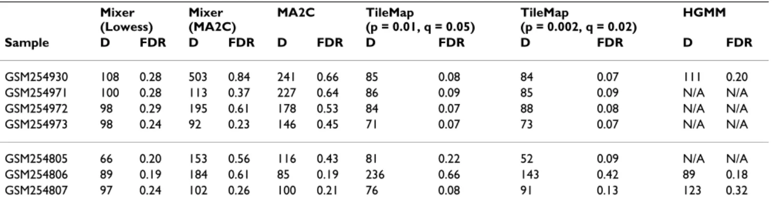
We then evaluated Mixer, MA2C, TileMap and HGMM using the spike-in data. First, given a fixed cutoff of either FDR ≤ 0.20 (for MA2C) or lfdr ≤ 0.20 (for the other meth-ods), we compared the power and actual FDR of these methods (Tables 1, 2 and 3). The discovery of a peak region was counted as a true discovery (or a true positive) if its center was within a spike-in region; otherwise it was counted as a false discovery. Although an alternative com-parison would examine the top K peaks identified by dif-ferent methods, we based our comparison on fixed lfdr/
Table 1: Comparison of different methods for the original data set
Mixer (Lowess) Mixer (MA2C) MA2C TileMap (p = 0.01, q = 0.05) TileMap (p = 0.002, q = 0.02) HGMM Sample D FDR D FDR D FDR D FDR D FDR D FDR GSM254930 108 0.28 503 0.84 241 0.66 85 0.08 84 0.07 111 0.20 GSM254971 100 0.28 113 0.37 227 0.64 86 0.09 85 0.09 N/A N/A GSM254972 98 0.29 195 0.61 178 0.53 84 0.07 88 0.08 N/A N/A GSM254973 98 0.24 92 0.23 146 0.45 71 0.07 73 0.07 N/A N/A GSM254805 66 0.20 153 0.56 116 0.43 81 0.22 52 0.09 N/A N/A GSM254806 89 0.19 184 0.61 85 0.19 236 0.66 143 0.42 89 0.18 GSM254807 97 0.24 102 0.26 100 0.21 76 0.08 91 0.13 123 0.32
The first four samples, GSM254930, GSM254971, GSM254972, and GSM254973 were spiked with unamplified DNA, while the last three samples GSM254805, GSM254806, and GSM254807 were spiked with amplified DNA. Among the total of 385,149 probes, about 820 (~0.2%) of them are from spike-in regions. We did not obtain results of HGMM for some arrays (N/A) due to failure of function HGMM.
FDR. This approach is more relevant since the number of binding sites is typically unknown.
We compared the results of Mixer after data normaliza-tion by Lowess or by MA2C. For the original data when the spike-in regions are sparse, in general, Mixer performs much better with Lowess normalization than with MA2C normalization. Mixer with MA2C normalization often includes many false discoveries resulting in a high FDR (see Table 1). As spike-in regions become more abundant, the normalization method makes less difference (Table 2, 3). Dissection of the mixture distribution becomes easier with additional data to estimate the alternative distribu-tion, which may overcome the differences attributable to the normalization methods.
We then compared the performance of the peak detection algorithms on the original and augmented data sets. HGMM was computationally intensive, requiring more than 10 hours to analyze one array. In contrast, the other methods we tested completed the analysis of a single array in less than 10 minutes. With the original data, (i.e., no replicates and a small proportion of spike-in regions),
HGMM failed for four arrays due to errors in numerical optimization. Although the use of initial values other than the defaults may avoid such errors, we did not explore this due to the high computational cost. In the augmented data sets (with a larger proportion of spike-in regions), HGMM did not fail for any array. However, HGMM was often over-conservative missing 30–50% of spike-in regions (Table 2, 3).
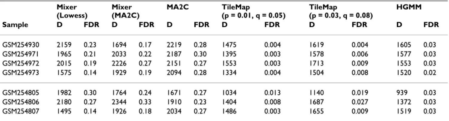
At the default parameters of p = 0.01 and q = 0.05 (i.e. using the top 1% of the data to estimate alternative distri-bution and 95% of the data to estimate null distridistri-bution), TileMap was over-conservative and had limited power, especially when the proportion of spike-in regions is high. TileMap performed much better when provided appropri-ate values for parameters p and q based on the true pro-portion of alternative distribution (Tables 1, 2 and 3). However, in actual applications, the alternative distribu-tion is typically unknown. For example, for amplified DNA samples when there are 4998 (~10.2%) spike-in regions, with lfdr smaller than 0.2, TileMap identifies ~70–80% of the spike-in regions if p = 0.08 and q = 0.13,
Table 2: Comparison of different methods for the simulated data set with 2,100/2,058 spike-in regions for unamplified/amplified samples, respectively Mixer (Lowess) Mixer (MA2C) MA2C TileMap (p = 0.01, q = 0.05) TileMap (p = 0.03, q = 0.08) HGMM Sample D FDR D FDR D FDR D FDR D FDR D FDR GSM254930 2159 0.23 1694 0.17 2219 0.28 1475 0.004 1619 0.004 1605 0.03 GSM254971 1965 0.21 2033 0.22 2187 0.30 1395 0.003 1578 0.006 1577 0.03 GSM254972 2015 0.19 2226 0.27 2151 0.27 1553 0.003 1713 0.009 1553 0.03 GSM254973 1575 0.14 1929 0.19 2094 0.28 1334 0.004 1504 0.008 1520 0.02 GSM254805 1982 0.30 1764 0.24 1671 0.27 1034 0.013 1140 0.019 939 0.03 GSM254806 2180 0.27 2344 0.33 1910 0.23 1404 0.008 1687 0.027 1372 0.03 GSM254807 1495 0.14 1926 0.18 2034 0.27 1486 0.003 1655 0.009 1519 0.03
See main text for the simulation methods. Approximately 4.3% of the probes are from spike-in regions.
Table 3: Comparison of different methods for the simulated data set with 5,100/4,998 spike-in regions for unamplified/amplified samples, respectively Mixer (Lowess) Mixer (MA2C) MA2C TileMap (p = 0.01, q = 0.05) TileMap (p = 0.08, q = 0.13) HGMM Sample D FDR D FDR D FDR D FDR D FDR D FDR GSM254930 4359 0.16 5753 0.28 4829 0.19 2775 0.001 3872 0.003 3707 0.02 GSM254971 4969 0.23 5110 0.23 4697 0.22 2758 0.001 3682 0.005 3615 0.02 GSM254972 5135 0.22 3957 0.19 4738 0.19 2978 0.001 4114 0.011 3558 0.03 GSM254973 4714 0.18 4795 0.20 4560 0.20 2695 0.001 3534 0.003 3493 0.02 GSM254805 4537 0.25 4784 0.27 3860 0.22 1946 0.003 2744 0.022 2237 0.03 GSM254806 4878 0.21 5826 0.32 4284 0.17 2672 0.0004 3924 0.022 3085 0.03 GSM254807 4957 0.21 5157 0.24 4569 0.20 2487 0.0004 3802 0.003 3508 0.02
but only ~60% of the spike-in regions with the default parameters, p = 0.01 and q = 0.05.
Both Mixer and MA2C have better power than TileMap and HGMM. As shown in Tables 1, 2 and 3, Mixer has lower FDR than MA2C for original data with sparse spike-in regions and has slightly better power than MA2C with abundant spike-in regions. However, a straightforward comparison between Mixer and MA2C is confounded by the fact that, unlike other methods, MA2C provides FDR estimates rather than lfdr estimates. Since lfdr and FDR cutoffs are not directly comparable, we employed ROC (receiver operating characteristic)-like curve to compare Mixer and MA2C (Figure 3). Unlike a typical ROC curve, these ROC-like curves plot (number of true positives)/ (number of spike-in clones) on the Y-axis against (number of false positives)/(number of spike-in clones) on the X-axis in order to accommodate the large number of true negatives in ChIP-chip data, [21]. To simplify the plots, we averaged across samples for amplified/unampli-fied DNA respectively. FDR and lfdr cutoffs were set between 0.01 to 0.50. Mixer outperformed MA2C when the spike-in regions were abundant (Figure 3). However, when the spike-in regions were sparse, MA2C outper-formed Mixer if an appropriate FDR cutoff was chosen.
Analysis of CTCF-binding Data
We also evaluated our method using the ChIP-chip data from a study of the zinc finger insulator protein CTCF (CCCTC-binding factor) in IMR90 human fibroblast cells[36]. This dataset includes 38 arrays each with about 38,500 50-mer probes tiling the non-repetitive sequences of the human genome in 100 bp resolution. The original pair data (pair data includes the intensities for two chan-nels, Cy5 (CTCF ChIP sample) and Cy3 (input genomic DNA)) were obtained from the Ren laboratory website http://bioinformatics-renlab.ucsd.edu/rentrac/wiki/CTCF _Project. Each of the 38 arrays was analyzed separately. The results of different peak-finding algorithms were com-pared to the results of an independent ChIP-seq based analysis that identified 20,262 CTCF binding sites in human CD4+ T cells [37].
HGMM was not evaluated due to its high computational cost. Model parameters were similar to those described above. For TileMap, window-level signals were summa-rized by HMM, and the lfdr of each peak region was esti-mated from unbalanced mixture subtraction (UMS) with default parameters (p = 0.01 and q = 0.05). For MA2C, default options were used to normalize data (robust with C = 2) and summary window-level signals (by median). In Mixer, the average DNA fragment length was set to 1500 bp (T. Kim, personal communication).
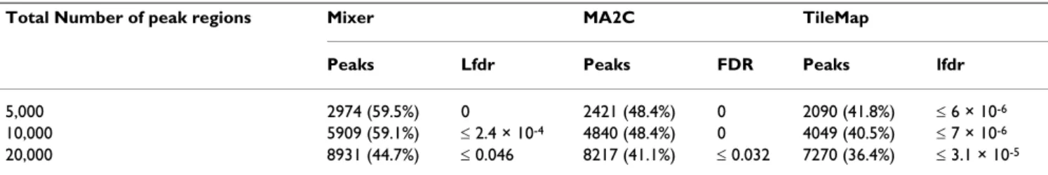
Although true CTCF binding sites are unknown, to permit a systematic evaluation of the various peak detection strat-egies, we compared the peak regions identified by each method with the 20,262 CTCF binding sites reported from a ChIP-seq study by Barski et al. [37]. Since experi-mental variation will likely result in differences between ChIP-chip and ChIP-seq data, ChIP-seq data serves as a common and independent source for comparison, rather than a perfect standard. A common site was called when the center of the ChIP-chip peak was located within the ChIP-seq peak. Without the knowledge of all true CTCF binding sites we are unable to compare FDRs, as we had done for the spike-in data. Therefore, we examined a fixed number of high confidence peak regions and compared the proportion of overlap. Specifically, we examined the overlap between the ChIP-seq reported sites and 5,000, 10,000, or 20,000 peak regions with the highest confi-dence (lowest FDR or lfdr) identified by each peak detec-tion algorithm. Peaks identified by Mixer consistently demonstrate a greater overlap with ChIP-seq peaks than those identified by MA2C and TileMap (Table 4).
Analysis of FAIRE Data
We also compared Mixer, MA2C, and TileMap on array data produced by hybridization of DNA enriched by For-maldehyde-Assisted Isolation of Regulator Elements (FAIRE)[19,38]. Briefly, FAIRE identifies open chromatin Comparison of Mixer and MA2C by ROC-like curves
Figure 3
Comparison of Mixer and MA2C by ROC-like curves.
Peaks were detected by Mixer (with Lowess normalization) or MA2C (with MA2C normalization). Some curves appear to be truncated at the left side because we restrict the cutoff to be FDR or lfdr smaller than 0.5. A larger cutoff is rarely used in practice.
regions using organic extraction of formaldehyde crosslinked chromatin. DNA recovered in the aqueous phase is fluorescently labeled and hybridized to arrays. FAIRE typifies the data from epigenetic studies where rel-evant features are expected to be abundant genome-wide. FAIRE-chip thus provides an appropriate application for Mixer. For this analysis, FAIRE was performed on chroma-tin isolated from human foreskin fibroblasts and hybrid-ized to a 1% ENCODE tiling array at 38-bp resolution [19].
Four arrays hybridized with FAIRE-selected chromatin were normalized individually. After averaging identical probes across the arrays Mixer was applied. MA2C and TileMap were run using their default options for replicate analysis. Since hypersensitivity to endonucleases is a standard method to identify open chromatin regions, we compared the results with 3,150 open chromatin regions identified by DNase I hypersensitivity-chip in lymphob-lastoid cell lines [39,40]. The FAIRE regions identified by each of the three methods share ~40% overlap with DNase sites, indicating similar specificities for the various methods. Since different techniques and different cell lines are compared, this overlap likely represents an underestimate of specificity. However, Mixer offers increased sensitivity as it identifies more peaks (especially those peaks with relatively weaker signals) at the same specificity. At a local FDR (for Mixer or TileMap) or FDR (for MA2C) cutoff of 0.2, Mixer identifies 1137 peaks (42.1% overlap with DNase hypersensitivity sites) whereas MA2C identifies 750 sites (43.3% overlap), and TileMap identifies 1114 sites (40.3% overlap). At a local FDR/FDR cutoff of 0.5, Mixer identifies 1559 peaks (40.3% overlap); MA2C identifies 1175 (39.7% overlap); and TileMap identifies 1202 (39.7% overlap).
A local FDR less than 0.5 is a much more stringent cutoff than FDR less than 0.5. The former means that the highest FDR for any one of the peak regions is 0.5, whereas the lat-ter indicates that the average FDR is 0.5. Averaging the local FDR less than 0.5 results in an estimated FDR for Mixer or TileMap of less than 0.15. Because it uses a less stringent FDR cutoff, MA2C is expected to identify more peaks. The actual identification of fewer peaks by MA2C
suggests the introduction of bias by MA2C normalization. To test this hypothesis, we supplied MA2C with Mixer-normalized data and observed a significant improvement of its sensitivity; 1,483 peaks (~40% overlap DNase sites) were identified at FDR less than 0.20, still fewer than the 1,559 peaks identified by Mixer with an estimated FDR of less than 0.15.
Discussion
We have developed a mixture model approach to dissect the mixture distributions of ChIP-chip data: the null dis-tribution (corresponding to the background signals) and the alternative distribution (corresponding to the ChIP-enriched signals), at both probe and window levels. This approach builds on the method of Buck et al. [5] to esti-mate null (background) distribution of ChIP-chip signal data and utilizes the Poisson point process assumption proposed by Zheng et al. [12] to model DNA fragmenta-tion. An advance over most existing peak detection strate-gies, our approach is less dependent on key assumptions and prior knowledge. Our method takes into account the auto-correlation structure of nearby probes, permits a rel-atively large proportion of ChIP-enriched signals in the mixture distribution, and does not require cross-array nor-malization. After dissecting the mixture distribution, both probe-level and window-level lfdrs are provided to evalu-ate the statistical significance of the identified peaks. Using three data set representing widely divergent experi-mental conditions, we demonstrated that our method performs comparably or better than several representative existing methods, especially when the true peak regions are abundant. Our method also applies Lowess fit data normalization to capture the non-linear relationship between log(Cy3) and log(Cy5) signals from two-color arrays. Mixer emphasizes the identification of abundant short peak regions rather than extended binding regions. We have recently developed a different method to identify broad signal patterns [31].
Despite Mixer's advances, areas for improved perform-ance remain. We smooth the lfdr estimate so that it decreases as probe-level/window-level signals increase. This smoothing strategy avoids major fluctuations of lfdr estimates when observations are limited (e.g. in tail
Table 4: Comparison of the peaks identified by Mixer, MA2C, and TileMap with sites identified by ChIP-seq.
Total Number of peak regions Mixer MA2C TileMap
Peaks Lfdr Peaks FDR Peaks lfdr
5,000 2974 (59.5%) 0 2421 (48.4%) 0 2090 (41.8%) ≤ 6 × 10⁻⁶
10,000 5909 (59.1%) ≤ 2.4 × 10⁻⁴ 4840 (48.4%) 0 4049 (40.5%) ≤ 7 × 10⁻⁶
20,000 8931 (44.7%) ≤ 0.046 8217 (41.1%) ≤ 0.032 7270 (36.4%) ≤ 3.1 × 10⁻⁵
In each cell, the number of overlapped peak regions and the percentage among the top k peak regions are shown, where k = 5,000, 10,000, or 20,000.
areas). A similar strategy has been used to define q-value from FDR estimates [32]. However, smoothing may lead to under-estimates of the lfdr, especially for small lfdr. To improve the lfdr estimates, both signal strength and signal pattern (for example the "triangle" pattern used by Zheng et al. [12]) could be incorporated, a strategy we are cur-rently evaluating.
The use of high throughput sequencing based chromatin identification (ChIP-seq) has become increasingly com-mon. However, determination of sufficient sequencing depth remains a significant challenge, especially for abun-dant epigenetic events. ChIP-chip remains a valuable method for pilot experiments and to cross validate results, a particularly appropriate application of Mixer. Mixer could also be adapted to dissect mixture distributions from sequencing data. Tag counts derived from unfrac-tionated input control could model a null distribution [41]. We are currently testing this approach.
Conclusion
In summary, we have developed a method that combines improved data normalization and peak detection for ChIP-chip studies. Mixer offers several advantages includ-ing lfdr determination and enhanced performance when peak regions are abundant, a common scenario for genome-wide studies of chromatin organization and epi-genetics [4,19,20].
Availability and requirements
We have implemented our method in an R package mixer, which can be freely downloaded from http:// www.bios.unc.edu/~wsun/software/mixer.htm. The source code can be redistributed and/or modified under the terms of the GNU General Public License as published by the Free Software Foundation.
Authors' contributions
All authors have read and approved the final manuscript. WS, IJD and MJB conceived this study. WS implemented the methods and analyzed the data. WS, IJD, MJB and MP wrote the paper.
Additional material
Acknowledgements
We thank Paul G. Giresi and Jason D. Lieb for providing the FAIRE data. WS is supported, in part, by the United States Environmental protection Agency grant (RD833825). However, the research described in this article has not been subjected to the Agency's peer review and policy review and therefore does not necessarily reflect the views of the Agency and no offi-cial endorsement should be inferred. IJD is supported in part by the National Cancer Institute (K08CA100400), the V Foundation for Cancer Research, the Rita Allen Foundation, and the Corn-Hammond Fund for Pediatric Oncology.
References
1. Ren B, Robert F, Wyrick JJ, Aparicio O, Jennings EG, Simon I, Zeitlin-ger J, Schreiber J, Hannett N, Kanin E, et al.: Genome-wide location and function of DNA binding proteins. Science 2000, 290(5500):2306-2309.
2. Lieb JD, Liu X, Botstein D, Brown PO: Promoter-specific binding of Rap1 revealed by genome-wide maps of protein-DNA association. Nat Genet 2001, 28(4):327-334.
3. Cawley S, Bekiranov S, Ng HH, Kapranov P, Sekinger EA, Kampa D, Piccolboni A, Sementchenko V, Cheng J, Williams AJ, et al.: Unbiased mapping of transcription factor binding sites along human chromosomes 21 and 22 points to widespread regulation of noncoding RNAs. Cell 2004, 116(4):499-509.
4. Kim TH, Barrera LO, Zheng M, Qu C, Singer MA, Richmond TA, Wu Y, Green RD, Ren B: A high-resolution map of active promot-ers in the human genome. Nature 2005, 436(7052):876-880. 5. Buck MJ, Nobel AB, Lieb JD: ChIPOTle: a user-friendly tool for
the analysis of ChIP-chip data. Genome Biol 2005, 6(11):R97. 6. Ji H, Wong WH: TileMap: create chromosomal map of tiling
array hybridizations. Bioinformatics 2005, 21(18):3629-3636. 7. Li W, Meyer CA, Liu XS: A hidden Markov model for analyzing
ChIP-chip experiments on genome tiling arrays and its appli-cation to p53 binding sequences. Bioinformatics 2005, 21(Suppl 1):i274-282.
8. Johnson WE, Li W, Meyer CA, Gottardo R, Carroll JS, Brown M, Liu XS: Model-based analysis of tiling-arrays for ChIP-chip. Proc
Natl Acad Sci USA 2006, 103(33):12457-12462.
9. Keles S, Laan MJ van der, Dudoit S, Cawley SE: Multiple testing methods for ChIP-Chip high density oligonucleotide array data. J Comput Biol 2006, 13(3):579-613.
10. Keles S: Mixture modeling for genome-wide localization of transcription factors. Biometrics 2007, 63(1):10-21.
11. Song JS, Johnson WE, Zhu X, Zhang X, Li W, Manrai AK, Liu JS, Chen R, Liu XS: Model-based Analysis of 2-Color Arrays (MA2C).
Genome Biol 2007, 8(8):R178.
12. Zheng M, Barrera LO, Ren B, Wu YN: ChIP-chip: data, model, and analysis. Biometrics 2007, 63(3):787-796.
13. Gottardo R, Li W, Johnson WE, Liu XS: A flexible and powerful bayesian hierarchical model for ChIP-Chip experiments.
Bio-metrics 2008, 64(2):468-478.
14. Benjamini Y, Hochberg Y: Controlling the false discovery rate: a practical and powerful approach to multiple testing. Journal of
the Royal Statistical Society, Ser B 1995, 57:289-300.
15. Efron B, Tibshirani R, Storey J, Tusher V: Empirical Bayes analysis of a microarray experiment. Journal of the American Statistical
Association 2001, 96:1151-1160.
16. Newton MA, Noueiry A, Sarkar D, Ahlquist P: Detecting differen-tial gene expression with a semiparametric hierarchical mix-ture method. Biostatistics 2004, 5(2):155-176.
17. Newton MA, Kendziorski CM, Richmond CS, Blattner FR, Tsui KW: On differential variability of expression ratios: improving sta-tistical inference about gene expression changes from microarray data. J Comput Biol 2001, 8(1):37-52.
18. Mardis ER: ChIP-seq: welcome to the new frontier. Nat
Meth-ods 2007, 4(8):613-614.
19. Giresi PG, Kim J, McDaniell RM, Iyer VR, Lieb JD: FAIRE (Formal-dehyde-Assisted Isolation of Regulatory Elements) isolates active regulatory elements from human chromatin. Genome
Res 2007, 17(6):877-885.
20. Wang Z, Zang C, Rosenfeld JA, Schones DE, Barski A, Cuddapah S, Cui K, Roh TY, Peng W, Zhang MQ, et al.: Combinatorial patterns of histone acetylations and methylations in the human genome. Nat Genet 2008, 40(7):897-903.
Additional File 1
Supplementary Materials for "Improved ChIP-chip analysis by mix-ture model approach". Supplementary results demonstrating different data normalization methods.
Click here for file
[http://www.biomedcentral.com/content/supplementary/1471-2105-10-173-S1.pdf]
Publish with BioMed Central and every scientist can read your work free of charge "BioMed Central will be the most significant development for disseminating the results of biomedical researc h in our lifetime."
Sir Paul Nurse, Cancer Research UK Your research papers will be:
available free of charge to the entire biomedical community peer reviewed and published immediately upon acceptance cited in PubMed and archived on PubMed Central yours — you keep the copyright
Submit your manuscript here:
http://www.biomedcentral.com/info/publishing_adv.asp
BioMedcentral 21. Johnson DS, Li W, Gordon DB, Bhattacharjee A, Curry B, Ghosh J,
Brizuela L, Carroll JS, Brown M, Flicek P, et al.: Systematic evalua-tion of variability in ChIP-chip experiments using predefined DNA targets. Genome Res 2008, 18(3):393-403.
22. Berger JA, Hautaniemi S, Jarvinen AK, Edgren H, Mitra SK, Astola J: Optimized LOWESS normalization parameter selection for DNA microarray data. BMC Bioinformatics 2004, 5:194. 23. Workman C, Jensen LJ, Jarmer H, Berka R, Gautier L, Nielser HB,
Saxild HH, Nielsen C, Brunak S, Knudsen S: A new non-linear nor-malization method for reducing variability in DNA microar-ray experiments. Genome Biol 2002, 3(9):research0048. 24. Yang YH, Dudoit S, Luu P, Lin DM, Peng V, Ngai J, Speed TP:
Nor-malization for cDNA microarray data: a robust composite method addressing single and multiple slide systematic vari-ation. Nucleic Acids Res 2002, 30(4):e15.
25. Buck MJ, Lieb JD: ChIP-chip: considerations for the design, analysis, and application of genome-wide chromatin immu-noprecipitation experiments. Genomics 2004, 83(3):349-360. 26. R Development Core Team: R: A language and environment for
statistical computing. 2007 [http://www.R-project.org]. Vienna, Austria R Foundation for Statistical Computing
27. Silverman BW: Density Estimation. London: Chapman and Hall; 1986.
28. Savitzky A, Golay MJE: Smoothing and Differentiation of Data by Simplified Least Squares Procedures. Anal Chem 1964, 36(8):1627-1639.
29. Steinier J, Termonia Y, Deltour J: Smoothing and differentiation of data by simplified least square procedure. Anal Chem 1972, 44(11):1906-1909.
30. Press WH, Flannery BP, Teukolsky SA, Vetterling WT: Numerical Recipes in C, The Art of Scientific Computing. 2nd edition. Cambridge University Press; New York City, NY; 1992.
31. Sun W, Xie W, Xu F, Grunstein M, Li K-C: Dissect nucleosome free regions by a segmental semi-Markov model. PLoS ONE 2009, 4(3):e4721.
32. Storey JD, Tibshirani R: Statistical significance for genomewide studies. Proc Natl Acad Sci USA 2003, 100(16):9440-9445. 33. Fejes AP, Robertson G, Bilenky M, Varhol R, Bainbridge M, Jones SJ:
FindPeaks 3.1: a tool for identifying areas of enrichment from massively parallel short-read sequencing technology.
Bioinformatics 2008, 24(15):1729-1730.
34. The ENCODE (ENCyclopedia Of DNA Elements) Project.
Science 2004, 306(5696):636-640.
35. Ji H, Jiang H, Ma W, Johnson DS, Myers RM, Wong WH: An inte-grated software system for analyzing chip and ChIP-seq data. Nat Biotechnol 2008, 26(11):1293-1300.
36. Kim TH, Abdullaev ZK, Smith AD, Ching KA, Loukinov DI, Green RD, Zhang MQ, Lobanenkov VV, Ren B: Analysis of the verte-brate insulator protein CTCF-binding sites in the human genome. Cell 2007, 128(6):1231-1245.
37. Barski A, Cuddapah S, Cui K, Roh T-Y, Schones DE, Wang Z, Wei G, Chepelev I, Zhao K: High-Resolution Profiling of Histone Meth-ylations in the Human Genome. Cell 2007, 129(4):823-837. 38. Giresi PG, Lieb JD: Isolation of active regulatory elements from
eukaryotic chromatin using FAIRE (Formaldehyde Assisted Isolation of Regulatory Elements). Methods 2009 in press. 39. Crawford GE, Davis S, Scacheri PC, Renaud G, Halawi MJ, Erdos MR,
Green R, Meltzer PS, Wolfsberg TG, Collins FS: DNase-chip: a high-resolution method to identify DNase I hypersensitive sites using tiled microarrays. Nat Methods 2006, 3(7):503-509. 40. Sabo PJ, Kuehn MS, Thurman R, Johnson BE, Johnson EM, Cao H, Yu
M, Rosenzweig E, Goldy J, Haydock A, et al.: Genome-scale map-ping of DNase I sensitivity in vivo using tiling DNA microar-rays. Nat Methods 2006, 3(7):511-518.
41. Rozowsky J, Euskirchen G, Auerbach RK, Zhang ZD, Gibson T, Bjorn-son R, Carriero N, Snyder M, Gerstein MB: PeakSeq enables sys-tematic scoring of ChIP-seq experiments relative to controls. Nat Biotechnol 2009, 27(1):66-75.