University of Windsor University of Windsor
Scholarship at UWindsor
Scholarship at UWindsor
Electronic Theses and Dissertations Theses, Dissertations, and Major Papers
2017
Rigorous Design of a Compact, Low-Speed, Open-Loop Wind
Rigorous Design of a Compact, Low-Speed, Open-Loop Wind
Tunnel
Tunnel
Kharuna Ramrukheea University of Windsor
Follow this and additional works at: https://scholar.uwindsor.ca/etd
Recommended Citation Recommended Citation
Ramrukheea, Kharuna, "Rigorous Design of a Compact, Low-Speed, Open-Loop Wind Tunnel" (2017). Electronic Theses and Dissertations. 6011.
https://scholar.uwindsor.ca/etd/6011
Rigorous Design of a Compact, Low-Speed,
Open-Loop Wind Tunnel
by
Kharuna Ramrukheea
A Thesis
Submitted to the Faculty of Graduate Studies
through the Department of Mechanical, Automotive & Materials Engineering in Partial Fulllment of the Requirements for
the Degree of Master of Applied Science at the University of Windsor
Windsor, Ontario, Canada
2017
Rigorous Design of a Compact, Low-Speed,
Open-Loop Wind Tunnel
by
Kharuna Ramrukheea
APPROVED BY:
D. Green
Department of Mechanical, Automotive & Materials Engineering
G. Rankin
Department of Mechanical, Automotive & Materials Engineering
J. Defoe, Advisor
Department of Mechanical, Automotive & Materials Engineering
Declaration of Previous Publication
This thesis includes one original paper that has been accepted for publication in conference proceedings, as follows:
Thesis Chapter
Publication title/ full citation Publication
status
Chapter 2, 3, 4,
and 6
A First Principles-Based and Numerical Design Approach for Fluid Flow Systems with Application to an Open-Loop
Wind Tunnel. Ramrukheea, K., Defoe, J. Proceedings of the 25thAnnual Conference of the Computational Fluid Dynamics Society of Canada, Windsor, ON, Canada, June
18-20, 2017.
Accepted
I certify that I have retained copyright to the above material in my thesis. I certify that the above material describes work completed during my registration as a graduate student at the University of Windsor.
I declare that, to the best of my knowledge, my thesis does not infringe upon anyone's copyright nor violate any proprietary rights and that any ideas, techniques, quotations, or any other material from the work of other people included in my thesis, published or otherwise, are fully acknowledged in accordance with the standard referencing practices. Furthermore, to the extent that I have included copyrighted material that surpasses the bounds of fair dealing within the meaning of the Canada Copyright Act, I certify that I have obtained a written permission from the copyright owner to include such material(s) in my thesis.
Abstract
Currently available literature regarding the design of uid ow systems tend to focus on the specic system without providing a general guideline for how to address the design problem. This thesis focuses on developing such a general approach which is applied to the design of a wind tunnel meant for the University of Windsor. It is shown that, by applying the rst principles of uid mechanics to the problem, the components required, for operation of the wind tunnel within set constraints and requirements are identied. Numerical simulations are performed in two parts: 1) two-dimensional computational uid dynamics simulations, which enable a paramet-ric study of each component, and 2) three-dimensional computations, which provide a more accurate estimation of the performance of the wind tunnel. By following these steps, it is found that computational cost is greatly reduced by rst sizing the components during the parametric study. The metrics used to assess the wind tun-nel performance are the ow non-uniformity and the total pressure loss coecient throughout the tunnel. The rst principles based approach yields a set of compo-nents, respecting the constraints set while two-dimensional computations allows the determination of the wind tunnel dimensions and estimation of its performance, which is veried by a three-dimensional computation.
Employing this approach, a successful wind tunnel design rated with a maximum volume ow rate of12.9m3/sat a test section inlet velocity of40m/s with the ability
to be attached to dierent test sections is achieved. This wind tunnel comprises a fan followed by a constant area duct leading to a diuser, which is attached to a ow conditioner. The last component is a nozzle directing the ow into the test section. The wind tunnel operates with an estimated 8% ow non-uniformity at the nozzle
exit together with a total pressure loss coecient of 0.238 based on the test section
Acknowledgements
Words cannot express my gratitude towards my supervisor, Dr. Je Defoe, who has shown unlimited patience and encouragement throughout this project. Under his supervision, I have been able to acquire and enhance my knowledge in the eld of computational uid dynamics (CFD), all while adopting a more ecient thinking process in solving problems. I am very grateful for his training that has helped me develop skills at both a personal and a professional level.
Undoubtedly, this project would not be possible without the help of many, such as Mr. Andrew Jenner, who constantly assisted and provided advice from the beginning to the end of this project. I would like to also extend my thanks to Mrs. Angela Haskell who has provided support on several occasions.
A special thank you goes to all my colleagues in the Computational Fluid Dynam-ics Laboratory who have helped me understand and face the many diculties in the CFD eld. I want to thank Mr. Kohei Fukuda, Mr. Ravinder Gill, Mr. David Hill, and Mr. Krishna Patel for their continuous feedback. I am indebted to Dr. Gary Rankin, Mr. Sichang Xu, and Mr. Chris Peirone who were kind enough to allow me to use their computer resources.
Contents
Declaration of Previous Publication iii
Abstract iv
Acknowledgement v
List of Figures ix
List of Tables xi
Nomenclature xii
1 Introduction 1
1.1 Objectives . . . 1
1.2 Introduction to the Wind Tunnel . . . 2
1.2.1 Requirements . . . 2
1.2.2 Constraints . . . 5
1.2.3 High Level Wind Tunnel Features to Address The Requirements and Constraints . . . 5
1.3 Challenges . . . 6
1.4 Key Outcomes . . . 7
2 Literature Review 9
2.1 Established Design Approaches for Specic Fluid Flow Systems . . . 9
2.2 Classication of Wind Tunnels . . . 11
2.3 Complete Wind Tunnel Design . . . 12
2.3.1 Fan . . . 12
2.3.2 Diuser . . . 13
2.3.3 Flow Conditioner . . . 17
2.3.4 Nozzle . . . 18
2.3.5 Implementation of CFD to Capture Fluid Flow Behaviour . . 20
2.3.6 Metrics for Wind Tunnel Performance Assessment . . . 21
2.4 Wind Tunnel Commissioning . . . 22
2.5 Aspects of the Literature Used in this Study . . . 23
3 Approach 25 3.1 First Principles Analysis of Flow within Wind Tunnel . . . 26
3.1.1 Study of Limiting Cases . . . 26
3.1.2 Fan Selection . . . 27
3.1.3 Fan Outlet Duct Requirement . . . 29
3.1.4 Diuser to Reduce Fan Outow Velocity . . . 30
3.1.5 Flow Straightener to Reduce Secondary Flows . . . 32
3.1.6 Nozzle Reducing Flow Non-Uniformity Entering Test Section . 33 3.1.7 Summary of First Principles Analysis . . . 35
3.2 Two-Dimensional Computational Fluid Dynamics Analysis of Wind Tunnel . . . 35
3.2.1 Diuser . . . 36
3.2.2 Flow Straightener . . . 37
3.2.3 Nozzle . . . 37
3.2.5 Limitation of Two-Dimensional CFD Computations . . . 40
3.3 Three-Dimensional Computational Fluid Dynamic Analysis of Wind Tunnel . . . 40
3.4 Summary of Approach . . . 42
4 Results 43 4.1 Overview of Final Wind Tunnel Design . . . 43
4.2 Results of Parametric Study . . . 44
4.2.1 Diuser Length . . . 44
4.2.2 Number of Screens Required . . . 45
4.2.3 Location of Screens . . . 47
4.2.4 Flow Straightener . . . 50
4.2.5 Nozzle . . . 51
4.2.6 Summary of Two-Dimensional Results . . . 53
4.3 Results of Three-Dimensional CFD Calculations of Wind Tunnel . . 54
4.4 Summary of Results . . . 58
5 Implementation of Wind Tunnel 60 5.1 Additional Features of this Wind Tunnel . . . 60
5.2 Manufacturing of the Wind Tunnel . . . 62
5.3 Commissioning of the Wind Tunnel . . . 63
6 Conclusions and Recommendations 64 6.1 Summary . . . 65
6.2 Conclusions . . . 66
6.3 Recommendations for Future Work . . . 68
List of Figures
1-1 Linear cascade blade test section requiring large changes in ow
direction. . . 3
1-2 Schematic illustration of an annular cascade blade test section. . . . 4
1-3 Semi-free jet test section. . . 4
1-4 Free jet test section with ground platform to support test model. . . 4
2-1 Geometric parameters describing a two-dimensional diuser. . . 14
3-1 Flowchart illustrating approach. . . 25
3-2 High ow non uniformity at fan outlet. . . 26
3-3 Centrifugal fan performance curves and outlet dimensions. . . 29
3-4 Diuser to slow down ow. . . 31
3-5 Flow eld within a diuser. Left: ow non-uniformity accentuates; right: onset of ow separation. . . 32
3-6 Flow eld within a nozzle. Left: ow non-uniformity decreases; right: attened velocity prole near wall. . . 34
3-7 Geometry of two nozzles required. . . 34
3-8 Design concept based on rst principles analysis. . . 35
3-9 Flow separation for upper limit of diuser length. . . 36
3-10 Radii of curvature at nozzle inlet and outlet. . . 38
4-1 Wind tunnel assembly with the rectangular nozzle attached. . . 44
4-2 Wind tunnel assembly with the circular nozzle attached. . . 44
4-3 Impact of screens on ow in a wide-angle diuser. Top: ow separation with no screens; bottom: attached ow due to presence of screens. . . 46
4-4 Location for analysis about required number of screens. . . 47
4-5 Larger separation bubble with screen located at 0.590Ld. . . 48
4-6 Impact of honeycomb on RM S%downstream. . . 51
4-7 Test section inlet velocity proles. . . 52
4-8 Velocity eld for selected conguration in 2D CFD. . . 53
4-9 Velocity eld for selected conguration in 2D CFD and 3D CFD. . . 55
4-10 Nozzle outlet velocity contours for 3D cases. . . 56
4-11 Comparison of RM S%for 2D and 3D CFD. . . 57
4-12 Comparison of ω for 2D and 3D CFD. . . 57
4-13 Fan providing margin for additional total pressure drop. . . 59
5-1 Wind tunnel assembly for manufacturing. . . 61
5-2 Enhancement features of the wind tunnel. . . 62
5-3 Angled ange to hold screen. . . 62
5-4 Clamps and casters for easy assembly and disassembly of nozzle. . . 63
List of Tables
3.1 Breakdown of estimated total pressure drop for wind tunnel system. . 28 3.2 Porous jump specications. . . 39 3.3 Percentage change in RM S% at nozzle outlet relative to grid with
75,000 cells. . . 40
Nomenclature
Symbols
A cross-sectional area
C recovery coecient
D duct diameter
L length
U axial velocity
W width
dA dierential cross-sectional area
l fan outlet length
p static pressure
RM S% normalized root-mean-squared variation in velocity
s screen solidity
u velocity magnitude
w fan outlet width
dp dierential pressure
du dierential velocity magnitude
dx dierential duct axial length
κ screen pressure drop coecient
ρ density
ω total pressure loss coecient
θ half diusion angle
Subscripts
d diuser
f fan
h honeycomb
i component inlet
n nozzle
o component outlet
s1 rst screen
s2 second screen
t total quantity
ts test section
Superscripts
X mixed-out quantity
Abbreviations
MAME Mechanical, Automotive & Materials Engineering
RMS Root-Mean Square
CFD Computational Fluid Dynamics
CTA Constant Temperature Anemometry
PIV Particle Image Velocimetry
LDV Laser Doppler Velocimetry
RANS Reynolds-Averaged Navier Stokes
Chapter 1
Introduction
To support teaching and research work within the Aerospace Option at the University of Windsor's Mechanical, Automotive & Materials Engineering (MAME) Department, a new wind tunnel is required. Currently, the department houses two wind tunnels which cannot accommodate the types of test sections required for the targeted area of study, which is turbomachinery. This thesis focuses on carrying out the design work for the wind tunnel by developing and employing an approach based on the application of the rst principles of uid mechanics. The design of specic test sections is not part of the scope of this work. With limited space allocation for laboratory equipment, the challenge of this project lies in designing a compact wind tunnel which can produce maximum volume ow rate of12.9m3/s with a uniform ow of40m/s. With a Mach
number of0.118 at the test section inlet (the region of highest average velocity across
the entire wind tunnel) the ow can be considered incompressible.
1.1 Objectives
the analysis from rst principles of uid mechanics applied to the problem of designing a wind tunnel with turbomachinery cascade and other test sections. The aim of this approach is to simultaneously achieve (1) a low total pressure drop, which sets the power required to drive ow through the tunnel, for a given ow rate and (2) a high level of ow uniformity at the test section inlet/ wind tunnel outlet. The large variety of types of test sections envisioned for use with this tunnel renders it impractical for the thesis scope to include test section design. Therefore, the uniformity at the tunnel outlet/test section inlet is the key gure of merit for the ow.
1.2 Introduction to the Wind Tunnel
This wind tunnel will provide ow for turbomachinery cascade test sections, among others. Thus, considered as a mass ow generator, this facility must provide high quality ow to the test section inlet, with the exibility to accommodate dierent types of test sections. This section presents the constraints and requirements set for this wind tunnel design. An introduction to the dierent types of test sections allow the identication of required features of the tunnel.
1.2.1 Requirements
The wind tunnel must provide a maximum volume ow rate of 12.9 m3/s at a test
section inlet velocity (U¯X
ts,i ) of 40 m/s; the minimum test section inlet velocity is
about 0.5 ¯Uts,iX m/s. The maximum performance is set based on expected Reynolds
number and Mach number for the envisioned test sections. The maximum volume ow rate and corresponding maximum velocity sets the outlet area of the wind tunnel to be An,o = 0.326m2. This combination of length and velocity scales yields test section Reynolds numbers on the order of2×105, sucient to ensure rapid turbulence
The ow non-uniformity present at the nozzle outlet is evaluated by an area-weighted normalized root-mean square (RMS) variation in velocity, RM S%. The full
denition of this parameter is given in section 2.3.6; based on the literature, it should not exceed 10% at the nozzle outlet.
The tunnel needs to accommodate dierent types of test sections, including both internal and external ows. The types of test sections already envisioned include: 1) turbomachinery blade cascades, 2) semi-free jets, and 3) free jets. A brief discussion of the characteristics of each of these types of test sections follows.
Blade cascades are a long-standing tool for assessment of turbomachinery blade performance and in aerodynamics research[1]. A cascade consists of a stationary row of equally-spaced blades, which can be categorised as either linear or annular depending on the blade arrangements.
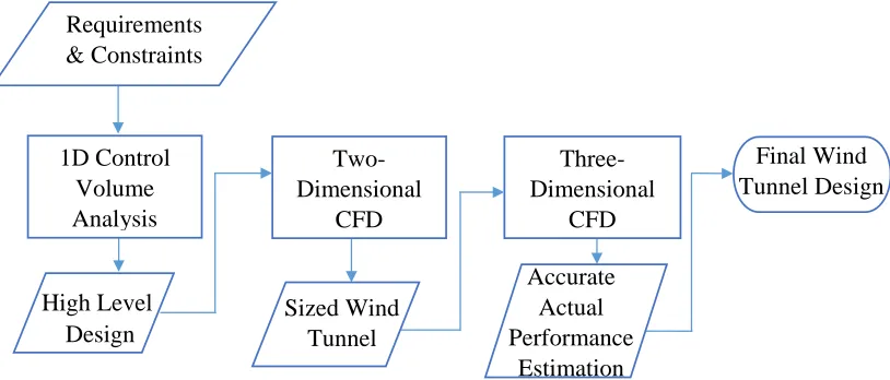
In a linear cascade, the blades are arranged in a straight line and the ow is turned by the blades as seen in Fig. 1-1. The turning angle may be large, possibly more than 90◦ for turbine blades.
Figure 1-1: Linear cascade blade test section requiring large changes in ow direction.
Figure 1-2: Schematic illustration of an annular cascade blade test section.
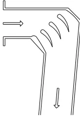
Enclosed test sections for assessing the performance of isolated airfoils can be limited in the amount of camber and/or the range of angles of attack available due to the presence of endwalls above and below the airfoil. The solution is to use a semi-free jet, as depicted in Fig. 1-3. The uid can exit the test section at the top and bottom in addition to the usual test section outlet.
No bottom wall
High angles of attack
Test section inflow
No top wall
Figure 1-3: Semi-free jet test section.
Free jets can be used to measure aerodynamic forces on bodies smaller than the jet diameter. By means of a ground support, the body of interest is placed in the tunnel outow jet, as illustrated in Fig. 1-4.
Ground support for test model
The requirements of the tunnel can thus be summarized as follows:
1. There is a need to accommodate dierent types of test sections, including both internal and external ows.
2. Due to the variety in test sections, the wind tunnel will need to match circular test section inlet for annular cascades and free jets, and the rectangular cross-sections of linear cascades and semi-free jet test cross-sections.
3. The dierence in direction between the inow and the outow of a test section can be larger than 90◦.
1.2.2 Constraints
The space occupied by the wind tunnel is limited by the room allocated, which is 13.4m long, 3.3m wide and 3.6m high. The total pressure drop through the passive components of the tunnel should be less than or equal to one fan outlet dynamic pres-sure. This limit is set based on the probable fan outlet velocity (0.5 ¯UX
ts,i), according
to a survey of potential fans for this application, all while considering the estimated allowable total pressure drop that will be incurred when driving the the ow through the test section.
1.2.3 High Level Wind Tunnel Features to Address The
Re-quirements and Constraints
Based on the requirements and constraints set, some of the features of the wind tunnel can be determined. First, an open-loop wind tunnel is selected to simultaneously address the issues of 1) limited space and 2) the requirement for the ow to undergo a turning of more than 90◦ in the test section. Unlike a closed-loop wind tunnel, an
this project. Including a test section, in which ow would undergo a large amount of turning, would be challenging and costly for a closed-loop wind tunnel.
It is also less expensive to accommodate dierent test sections within an open-loop wind tunnel. To match the dierent test section inlet geometries, only the upstream component of the test section needs to be duplicated in the case of an open-loop wind tunnel. Within a closed loop wind tunnel, both the upstream and downstream components of the test section would need to be replicated to match the inlet and outlet of the test sections.
Within an open-loop wind tunnel, a pusher style fan or a suction conguration can be used to drive the ow. With the former option, the ow is driven into the test section, located downstream of the fan. In the suction style, air is drawn into the test section from the environment. A suction fan would require separate bellmouth inlets to draw air into the tunnel for each type of test section used.
To address the variety of possible test sections, some type of adaptation is re-quired to accommodate both round and rectangular test section inlets. The largest allowable cross section of the wind tunnel is2.0m wide by2.0m high due to clearance
requirements. The maximum length of the tunnel, including the fan, is restricted to
7.8m to ensure adequate space is allocated for the test section.
1.3 Challenges
The compact nature of the wind tunnel requires a rigorous design process to simultaneously achieve high ow uniformity and low losses. Another challenge of this project is to establish a wind tunnel design with an overall geometry simple enough to manufacture.
1.4 Key Outcomes
The key outcomes of this thesis are:
1. A design approach which can be applied to other uid ow systems is devel-oped. This approach involves applying the rst principles of uid mechanics to the design problem to identify the dierent components required to satisfy the constraints and requirements set. This is followed by numerical compu-tations which are performed in two stages. Two-dimensional computational uid dynamics (CFD) computations are employed in a parametric study of each component to determine the best geometry with respect to the gures of merit. Three-dimensional CFD computations are carried out to provide a more accurate estimation of the performance of the complete, sized wind tunnel.
2. A fully operational open-loop subsonic wind tunnel addressing the requirements and constraints, has been installed within the MAME department at the Uni-versity of Windsor. The wind tunnel is predicted to provide a ow with non-uniformity of 8.07% all while keeping the total pressure drop at 0.238 times
the test section inlet dynamic pressure. Equipped with a pusher type fan, it can provide a maximum volume ow rate of 12.9 m3/s at a test section inlet
velocity of40m/s. It also comprises two nozzles, which can easily be mounted,
to deal with the dierent test sections.
1.5 Scope of Thesis
Chapter 2
Literature Review
This chapter presents relevant past work in the eld of uid ow system design. The focus is on wind tunnels and common components of such equipment. The metrics used to evaluate the performance of the wind tunnel, as well as previous work done in assessing wind tunnel performance are also reviewed. The shortcomings of the presented studies are also identied.
2.1 Established Design Approaches for Specic Fluid
Flow Systems
Several studies present design approaches for dierent specic uid ow systems such as work done by Vivek et al. [2], where CFD is applied in the design of the main vessel cooling system for pool-type fast nuclear reactors. Detailed parametric studies regarding the turbulence models which can be used concluded that the k −ε
is validated by comparing the results obtained from the calculations, when applied to the main vessel cooling circuit of a Japanese reactor, to those obtained during experiments found in the open literature. Two-dimensional CFD successfully allowed the determination of the amount of sodium ow rate required to maintain a certain main vessel temperature, while three-dimensional CFD enabled the discovery of how the manufacturability of an oval structure aects the circumferential temperature dif-ference in the main vessel. This study is successful in illustrating how a CFD based approach can be used to model and design a main vessel cooling system. Yet, by focusing only on the cooling system's features without providing a general guideline of how this approach can be applied to other systems, it is representative of that found in the literature in that the approach is applicable to only a narrow class of problems. This thesis is based on a general approach, which can be applied to other design problems.
description of the design approach adopted for a wind tunnel, it is limited to closed-loop wind tunnels. The requirements for the current wind tunnel to accommodate test sections with a wide variety of turning angles necessitates an open-loop design and thus precludes the use of the authors' approach.
The work presented by Mehta [4] describes general design rules of several compo-nents for a blower type wind tunnel. These rules are based on a review of the layout and performance of wind tunnels developed up to that point. The work is focused on wide-angle diusers, the use of screens within them, and centrifugal blowers. Section
2.3discusses how these rules, which have been derived by the author, aect the design of each component. While this is a good resource to start with, the fact that this paper is based on dierent wind tunnels which were known to have performed satis-factorily up to that point (1979) implies that there could be more up-to-date studies about the matter. For example, limited computational resources available restricted researchers' ability to fully investigate the uid ow within the wind tunnel. They could only assess the performance of a wind tunnel based on experiments, and were focused on one aspect of the wind tunnel at a time, due to the time-consuming aspect of experimental work. Therefore, this thesis aims at enhancing the literature by pro-viding a design approach based on the analysis of rst principles of uid mechanics and CFD calculations.
2.2 Classication of Wind Tunnels
tunnel is simpler than that of a closed-loop one, the latter reduces the power required to drive a given ow rate [5]. An open-loop conguration raises concerns with respect to noise treatment required to prevent any environmental problems [6]. Yet, since this setup provides more exibility with regards to the varying test section geometry, the need for an open-loop wind tunnel is re-armed.
2.3 Complete Wind Tunnel Design
This section is divided in six parts with focus on the dierent common components of a wind tunnel, the use of CFD in designing a wind tunnel, and the metrics used throughout this thesis to assess the performance of the wind tunnel.
2.3.1 Fan
Cattafesta et al. [7] indicate that fans and compressors are the two primary drive systems for a wind tunnel. To drive air through a wind tunnel, a compressor can be used to provide pressurised air from a storage tank. Alternatively, a fan, which can be axial or centrifugal, drives air through the wind tunnel by pushing or pulling it through the test section. The main advantage fans hold over the compressors is the ability to continuously provide air to the test section. The latter can only provide a xed amount of air, restricted by the storage tank's capacity, which limits the duration of an experiment.
thus making it an ideal candidate to run an open-loop wind tunnel.
Bradshaw [8] describes how the outow from a centrifugal fan is far from uniform. This ow phenomenon is mainly due to the span of the rotor being only half of the width of the volute casing, a feature that the manufacturers used to match the blower characteristics to a typical low-velocity ventilating system without using a long conical diuser. By investigating the ow within a wind tunnel, which is meant to provide low-turbulence ow with or without a diuser, the author found that with adequate use of screens and a ow conditioner, the non-uniformities can be eliminated. Yet, it is emphasized that non-uniform ow from the blower, notably the presence of thick boundary layers, can lead to separation and thus increase the losses and ow unsteadiness within a wide-angle diuser. Available literature [7, 4, 8] indicates that a centrifugal fan is an excellent candidate for an open-loop wind tunnel. Since no accurate prediction of the outow from the fan is available, this thesis provides measures that can be implemented to address the potential, harmful non-uniformities at the outlet of centrifugal fans.
2.3.2 Diuser
asymmetry and unsteadiness. Mehta [4] identies that another feature that can lead to ow separation is the presence of sharp inlet corners; by lleting these corners, this problem can be avoided.
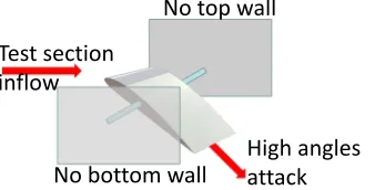
The eect of ow separation in diusers has been extensively studied; Reneau et al. [10] describe the four regimes of uid ow within which a two-dimensional diuser (with expansion between only one pair of walls) can fall. These four regimes, separated and indicated by means of a diuser stability map, are empirically based on water table studies in which dye injection is used to visualize the ow behaviour within diusers [11, 12, 13, 14]. These regions were veried when similar experiments were performed with air as a uid by Reneau et al. [10], Cochran et al. [12], Feil [13], and Johnston et al. [14]. This diuser stability map identies the geometrical constraints for which ow within a planar diuser can reach better pressure recovery with slightly separated ow. The constraints of importance in this case are the diusion angle, 2θ,
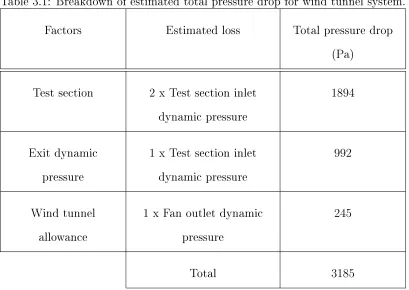
and the diuser axial length to inlet width ratio, Ld/Wd,i; the combination of these two parameters indicates the regime within which a diuser, as illustrated in Fig. 2-1, will operate.
𝑊𝑑,𝑖
𝐿𝑑
2𝜃
Figure 2-1: Geometric parameters describing a two-dimensional diuser.
The No Appreciable Stall regime comprises diusers with angles of diusion of no more than 22. Within this area of the chart, it is still possible to observe small
Within the Large Transitory Stall regime, the region of separation continuously appears on either of the two diverging walls; while in the Two-Dimensional Stall regime, the separation occurs near the throat and follow only one diverging wall. The Jet Flow regime is one within which ow separation occurs along both diverging walls, originating from the throat area. While this study assists in designing a diuser while avoiding the occurrence of separation, it presents a considerable limitation in that it is only applicable to planar diusers. For the purpose of this thesis, the diuser stability map is used to locate the regime within which the designed diuser lies, thus limiting this wind tunnel design to the use of a planar diusers.
Two types of diusers commonly referred to are the exit diuser and the wide angle diuser [9, 4, 6]. As the name suggests, the exit diuser is located downstream of the test section with a `gentle' expansion of no more than 5◦-10◦. This diuser
is implemented to reduce the dynamic pressure of the jet, hence lowering the total pressure loss, that is released at the end of the tunnel. Yet, for ease of changing test sections, and to keep a wind tunnel as compact as possible, this component tends to be omitted.
regions of contraction and sudden expansion to mix out the ow; and vanes which can guide the inlet ow to improve diuser performance. Compared to the listed options, Mehta and Bradshaw [9] established that the most common option used for economical reasons is the use of mesh screens.
As discussed by Greitzer [15], screens energize the boundary layer to delay the onset of ow separation. The presence of screens within a wind tunnel system leads to additional total pressure losses. The total pressure drop associated with a screen is determined using equation 2.1 given by Greitzer. This total pressure drop is related to its solidity ratio and velocity as follows:
∆pt=
1 2κρu
2 (2.1)
whereρis the uid density, uis the ow velocity magnitude, and κis the screen
pres-sure drop coecient, which can be determined using equation 2.2, given by Cornell [16]. This equation indicates how κ depends only on the screen solidity ratio s.
κ = 0.8s
(1−s)2 (2.2)
however, the pressure recovery is poor. It was also determined that two screens are sucient to achieve ow uniformity; however, in the case of an asymmetric diuser, an additional one is required. The ndings of the study presented by Noui-Mehidi are used for the design of a wide angle diuser with screens in this thesis.
2.3.3 Flow Conditioner
Cattafesta et al. [7] describe a ow conditioner as a duct section comprising a honey-comb, screens and a settling duct. When uid ows through the honeycomb structure, the ow is aligned with the axis of the tunnel and the large scale ow unsteadiness is broken into smaller scales. Screens then further decay these turbulent uctuations. To allow smaller scale ow unsteadiness to decay, a suciently long settling chamber is required while keeping the boundary layer growth to a minimum. Barlow et al. [6] indicate that compared to circular and square shaped cells, hexagonal cells are pop-ular due to their low pressure drop coecient. When compared to circpop-ular cells, the hexagonal cells are joined together at each of their vertex without creating any gaps. Also, according to Hales [19], a hexagonal grid leads to the least total perimeter when a surface is divided into regions of equal area, thus leading to less total pressure drop due to skin friction.
Barlow et al. [6] also indicate that the best performance of a honeycomb can be achieved when its length to cell hydraulic diameter ratio is in the range of 6-8. While these rules have been used in the design of wind tunnels, the authors do not deny the fact that these have originated from observations of many arrangements. Further, this range is based on assumptions that may or may not be valid for a particular wind tunnel application. Therefore, the validity of such rules can be questioned for dierent wind tunnel design.
respect to screen implementation downstream of the honeycomb, screens or honey-combs of large cross-sectional area are dicult to make suciently rigid. To cover the large surface area, screens have to be spliced together, which is accomplished by brazing the widths of the screens together. The irregularities that result from the brazing have the potential of introducing turbulence. Therefore, based on this re-view, it can be seen that a honeycomb coupled with a settling chamber is required, while the need for screens depends on the cross-sectional area across which they will be tted and the total pressure drop the screens will cause.
2.3.4 Nozzle
Several authors such as Cattafest et al. [7], Mehta and Bradshaw [4, 9], and Barlow et al. [6] agree that the nozzle is a critical wind tunnel component used to increase the mean velocity of the ow and to align the ow into the test section, thus de-termining the ow quality within the test section. As indicated by Morel [20], the acceleration achieved within the nozzle serves dierent purposes. For instance, due to the favourable pressure gradient within it, it is an aid to reduce the mean ow non-uniformities and to achieve a homogeneous ow at the test section inlet. Similarly, it scales down the turbulence level by breaking large scale eddies into small ones. In addition to achieving high ow uniformity and avoiding ow separation, minimum exit boundary layer thickness coupled with minimum contraction length are desirable attributes for a nozzle. The presence of wall curvature is required to avoid the risk of ow separation due to locally adverse pressure gradients near the walls; thus, a de-sign satisfying these criteria would ensure that separation is just avoided and that the exit non-uniformity presents a velocity variation of ±1
2% outside the boundary layer.
makes it a less realistic design.
Based on the assessment of the successful wind tunnels, Mehta [4] states that the nozzle contraction ratio should be between 6 and 9. Mehta and Bradshaw [9] state that a smooth ow of air through the nozzle exit is important, due to its impact on potential ow separation. Therefore, the overall shape of the nozzle does not matter as much as does the geometry near the nozzle exit. It is emphasized that the nozzle's curved section should smoothly join the parallel sections such that the rst and second derivatives of the curve at these meeting points are zero.
Nozzle design has been heavily inuenced by the work done by Morel [20], in which the author developed charts for wind tunnel contractions using an inviscid, incompressible ow analysis. The numerical approach, enforced with the use of a computer program of the streamline curvature type (developed by General Motors Detroit Diesel-Allison Division), focuses on the investigation of one commonly used group of wall nozzles with the shapes being dened by two cubic arcs smoothly joined. For dierent wall shapes, the wall pressure coecients at the inlet and outlet are calculated using equation 2.3, which is derived from the application of Bernouilli's equation given by equation 2.4.
Cp = 1−
Un,o
Un,i !2
(2.3)
p+1 2ρU
2 =constant (2.4)
aims at making use of this tool to design the nozzle without the restriction on the number of independent variables that can be studied at a time.
2.3.5 Implementation of CFD to Capture Fluid Flow Behaviour
When compared to experimental investigations, CFD simulation of the ow within a wind tunnel provides an inexpensive, in terms of time and money, estimation of the uid behaviour. To capture all ow behaviours within the wind tunnel accurately, the choice of turbulence model for the numerical calculations is critical, especially when ow separation is expected. An investigation carried out by Bardina et al. [21] showed that the Shear Stress Transport (SST) model by Menter [22] most accurately captures the details of separated ows. The authors compared and evaluated the performance of four popular turbulence models: the two equationk-ωmodel of Wilcox
[23], Launder and Sharma's [24] two equationk-model, the two equation SST model,
and the one equation Spalart-Allmaras model [25]. The evaluation was carried out by comparing against experimental data for ten turbulent ows. The application of these models to the case of a separated boundary layer, which was one of the turbulent ows investigated, led to the conclusion that the SST model is the best at capturing ow separation.
More recent work, such as that presented by Moonen et al., demonstrates how CFD is eective in predicting the ow behaviour within a wind tunnel [26]. The authors acknowledged the limited use of CFD in wind tunnel design; thus, the purpose of the study was to establish a methodology for numerically modelling the ow conditions in the full scale Jules Verne climatic closed-loop wind tunnel. Using a k- model,
The simulations were performed for two cases, one with an empty test section and the other comprised a test model in the test section. By comparing the CFD results to available experimental results, this methodology of modelling the entire wind tunnel provides velocity values with an error of no more than 10%. The author concluded that the accuracy of the results from simulating the full model was 2-4 times better than the conventional CFD analysis of the test section only. This paper provides a basis for implementing the use of CFD as a tool in wind tunnel design and testing.
2.3.6 Metrics for Wind Tunnel Performance Assessment
A key parameter for assessing wind tunnels is the test section inow uniformity. The metric used for this assessment of the wind tunnel performance is dened by Noui-Mehidi [17] as the normalized RMS variation in velocity dened in equation 2.5:
RM S% = 100
s U RM S ¯ UA 2
−1 (2.5)
where
URM S = v u u u t 1 A ˆ A
U2dA, (2.6)
and
¯ UA= 1
A
ˆ
A
U dA. (2.7)
U is the local ow velocity,U¯ is the area-averaged value of the local velocities normal
to a surface of cross-sectional areaA. Area-averaging is employed since it is the prole
of the velocity that is of concern. AnRM S%value of0represents a perfectly uniform
by
ωio =
¯ pX
t,i−p¯Xt,o
1 2ρ(U¯
X ts,i)2
(2.8)
wherep¯X
t is the mixed-out average total pressure across the cross-section at the
com-ponent inlet i and outlet o. Mixed-out averaging at constant area is used to capture
the additional eventual downstream loss rather than simply the local loss. This op-eration is dened in Greitzer et al. [15] for incompressible ow as
¯ pXt = 1
A
ˆ
A
pdA+ 1 A
ˆ
A
ρU2dA− 1
2ρ
¯
UX2 (2.9)
These metrics are used to evaluate the tunnel's performance at dierent locations. The RM S% provides an indication of the ow non-uniformity while ω gives a
non-dimensional indication of the total pressure drop; this is needed to know the required fan pressure rise.
2.4 Wind Tunnel Commissioning
Once these experiments are determined, the equipment required for these are established. For instance, to determine the ow uniformity, the velocity prole can be captured by measuring the values by traversing a Pitot static probe or a Pitot probe throughout the test section or more advanced equipment such as hot wires congured for constant temperature anemometry (CTA), particle image velocimetry (PIV), or laser doppler velocimetry (LDV) can be used.
Harvey [27] experimentally evaluated the performance of the Naval Postgraduate School Mechanical and Aerospace Engineering wind tunnel, which was re-installed and calibrated, to determine whether it was suitable for research and teaching pur-poses. With the use of pressure transducers attached to a Pitot static tube, wall static pressure taps, a pressure rake, and a hot wire anemometry system coupled with a rectangular traverse system, the author determined the wall static pressure distribution, total pressures across planes at dierent axial locations, the wall bound-ary layer characteristics, and the spectral energy distribution at selected points. With the help of a data acquisition processor with analog to digital conversion coupled with an in-house developed LabVIEW software, the author was able to determine that the new maximum axial speed was only 84% of the tunnel's rated speed. The ow uni-formity was determined to be within±7% of the mean freestream velocity with the
use of the pressure rake; the turbulence intensity was obtained within the range of 3%. An approach similar to the one described by Harvey is adopted for the planned commissioning of this wind tunnel.
2.5 Aspects of the Literature Used in this Study
Chapter 3
Approach
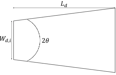
The design approach adopted for the wind tunnel is illustrated in Fig. 3-1. One-dimensional control volume analysis is employed to identify the required components. Based on the resulting components, a parametric study, using two-dimensional CFD computations, is performed to obtain nal dimensions of the components. Three-dimensional CFD calculations provide an enhanced estimation of the complete wind tunnel performance. A Computer Aided Design (CAD) model of the entire tunnel is then created to enable fabrication.
Requirements & Constraints
1D Control Volume Analysis
Two-Dimensional
CFD
Three-Dimensional
CFD
Final Wind TunnelDesign
High Level Design
Sized Wind Tunnel
Accurate Actual Performance
Estimation
3.1 First Principles Analysis of Flow within Wind
Tunnel
The following section summarises how the rst principles of uid mechanics are ap-plied to determine which components are required for this wind tunnel.
3.1.1 Study of Limiting Cases
An open-loop wind tunnel equipped with a pusher style fan leads to two limiting cases, which are 1) connecting the fan to the test section through a long duct to enable complete mixing and thus uniform test section inow, or 2) attaching the fan directly to the test section to minimize the pressure rise required. While these limiting cases could provide simple solutions to the problem, the constraints are such that the former option is impractical due to the allocated room's length of 13.4m.
Considering the space that is needed for the test section there needs to be a limit on the length of duct between the fan outlet and the test section inlet. For the case of the fan being directly connected to the test section, a high ow non-uniformity is expected to enter the test section, as seen in Fig. 3-2.
Inlet collar
Fan housing
Fan outlet duct
Figure 3-2: High ow non uniformity at fan outlet.
and the test section inlet. Since it is expected that the fan outlet and test section areas will dier, it can be established that some length of non-constant area duct is required.
3.1.2 Fan Selection
As suggested by Bradshaw[8], the volume ow rate and static pressure rise required to drive the air throughout the tunnel need to be dened to select a fan. With the maximum volume ow rate dened, the static pressure rise required to drive air throughout the wind tunnel is determined by estimating the total pressure loss for the wind tunnel and test section. The breakdown of the total pressure drop estimated for the wind tunnel is illustrated in Table 3.1. The total estimated loss is expressed in terms of the test section inlet dynamic pressure (= 1
2ρ( ¯U
X
ts,i)2 = 992 Pa). Since
Table 3.1: Breakdown of estimated total pressure drop for wind tunnel system.
Factors Estimated loss Total pressure drop
(Pa)
Test section 2 x Test section inlet dynamic pressure
1894
Exit dynamic pressure
1 x Test section inlet dynamic pressure
992
Wind tunnel allowance
1 x Fan outlet dynamic pressure
245
Total 3185
The total pressure of 3185 Pa represents3.25times the test section inlet dynamic
pressure. To account for any potential additional total pressure drop, a margin of
≈0.30test section inlet dynamic pressure is added to this estimate, leading to a total
estimated loss of 3484 Pa, which is approximately equal to 14 inWG. This pressure
rise required from the fan coupled with the volumetric ow rate of12.9m3/s are used
to select a potential fan from the manufacturer Northern Blower. As suggested by Mehta [4] and Bradshaw [8], a centrifugal fan with airfoil-type blades is chosen. The performance curve of the 5730 fan design (size 3650) together with a simple sketch of the fan, provided by Northern Blower [28], is seen in Fig. 3-3. The selected fan provides the maximum volume ow rate of 12.9 m3/s (27350 cubic feet per minute
(CFM)) with an outlet velocity of 0.504 ¯UX
ts,i through an outlet of dimensions of wby
Static Pressure 14”WG
BHP 76.75
Volume flow rate 27350 CFM
w
1.73w
Figure 3-3: Centrifugal fan performance curves and outlet dimensions.
3.1.3 Fan Outlet Duct Requirement
As sketched in Fig. 3-2, the fan outow is expected to exhibit high ow non-uniformity. To prevent the possibility of further increasing any losses in the stream component, a duct with same dimensions as the fan outlet is attached down-stream of the fan. Sugarman [29] indicates that for a fan outlet velocity of 12.7 m/s
or less, the length of the duct downstream of the fan outlet should be 2.5 times the duct diameter with one added duct diameter for each additional 5.1m/s in speed.
With the selected fan, the outow velocity is20.1m/s, implying the need for a duct
of length equal to four times the duct diameter. The duct diameter, D, is calculated
D=
s
4lw
π (3.1)
In this equation, l and w are the dimensions of the fan outlet. The required length
of the duct is found to be 5.93w, which is about 3.63 m, representing 46.7% of the
allowable length of the tunnel or 27.1% of the room's length. Since there is a need for space to accommodate more components, used to change speed of the ow and allow mixing of the uid ow before it reaches the test section, this length of duct is more than what can be used.
Referring to Fig. 3-2, as the duct length is increased, the outow from the fan outlet approaches a fully developed state, comprising a symmetric velocity prole. Therefore, in determining the length of this fan outlet duct, the aim is not to reach the fully developed velocity prole but rather provide sucient duct length to achieve a velocity prole which is at least near to symmetric. From the same gure, it is clear that the duct should be between 50% and 75% of the required length to achieve such a velocity prole. By considering the constraints and this factor, the maximum possible length of the duct is determined to be 66% of what is recommended, equal to 3.92w.
3.1.4 Diuser to Reduce Fan Outow Velocity
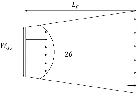
𝑊𝑑,𝑖
2𝜃 𝐿𝑑
Figure 3-4: Diuser to slow down ow.
To determine the fan dimension across which diusion will be considered (w or
1.73w), the No Appreciable Stall region of the diuser stability map is used to
ensure an analysis based on a diuser with no ow separation. For each of the two dimensions of the fan outlet, the ratio of Ld
Wd,i is calculated, and the corresponding diusion angles are obtained from the graph. It is determined that by expanding the duct across the shorter side, w, a larger area ratio, hence a lower ow velocity, is
obtained.
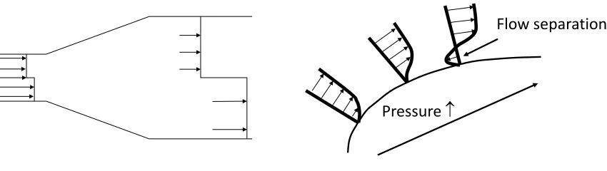
While a diuser is critical to allow mixing at low speed, it is at risk of two uid ow phenomenon. Given by equation 3.2, the velocity of a ow within a diuser depends on its acceleration and the pressure gradient across it. In the presence of ow non-uniformity, as seen from the left side of Fig. 3-5, with an increasing cross-sectional area in the streamwise direction, the ow slows down. For the same pressure gradient across the duct, slow ow has a larger deceleration du
udu dx =
1 ρ
dp
dx (3.2)
The other concern with a diuser is ow separation. In any ow, the ow near the wall travels at a slower speed, and thus can easily be aected by the adverse pressure gradient in a diuser. When this pressure gradient is large enough, the uid may show down to a zero velocity away from the wall or even become reversed. As seen in the right part of Fig. 3-5, this leads to ow separation.
Flow separation
Pressure
Figure 3-5: Flow eld within a diuser. Left: ow non-uniformity accentuates; right: onset of ow separation.
Analysis of the rst principles of uid mechanics enables the determination of which component is required downstream of the fan attached to the constant area duct; however, further investigation is required to determine the best dimensions for this diuser. Therefore, to determine the length, coupled with the diusion angle, two-dimensional CFD computations are required, as described later.
3.1.5 Flow Straightener to Reduce Secondary Flows
For the ideal case of a diuser with diusion angle of no more than 20◦ (no ow
non-uniformities due to ow separation, mixing enhancement required within a short distance can be achieved via a ow straightener.
As discussed by Barlow and Cattafest et al. [6, 7], a honeycomb is used to align the ow with the axis of the tunnel and to reduce secondary ows by breaking up large scale ow unsteadiness. This honeycomb is envisioned to comprise hexagonal cells due to its popularity with regards to low pressure drop.
Downstream of the honeycomb, a constant area duct is required to further break the small scale unsteadiness through the mixing of the jets and wakes. There is a restriction on the length of this duct due to boundary layer development. Screens within the ow straightener section are omitted due to the challenge of obtaining rigid ones for the large cross-sectional area.
Two-dimensional CFD calculations are required to determine the length of the ow straightener section for this wind tunnel. Further investigations are needed to establish the cell size of the honeycomb, as well as the length of the structure.
3.1.6 Nozzle Reducing Flow Non-Uniformity Entering Test
Section
Pressure
Thin boundary layer
Figure 3-6: Flow eld within a nozzle. Left: ow non-uniformity decreases; right: attened velocity prole near wall.
For this wind tunnel, two nozzles are required to accommodate circular and rect-angular cross-section test sections, as seen in Fig. 3-7, with both having the same outlet area. With respect to the nozzle design, the length is constrained with the space taken by the diuser and ow conditioner. One-dimensional analysis of the nozzle cannot capture ow non-uniformity introduced due to wall curvature in an aggressive nozzle. Therefore, a parametric study of 2D CFD computations is carried out to determine the shortest length with acceptable ow non-uniformity. The results of this study will be presented in section 4.2.
3.1.7 Summary of First Principles Analysis
From this analysis, a high-level design of the wind tunnel is established. The schematic of the wind tunnel, as seen in Fig. 3-8, comprises a constant area duct which connects the fan to the diuser, followed by a honeycomb coupled with a mixing chamber. The wind tunnel ends with a nozzle to accelerate the uid from the ow straightener to the test section.
Fan
Diffuser Honeycomb
Nozzle Test section
Duct at fan outlet
Mixing chamber
Figure 3-8: Design concept based on rst principles analysis.
3.2 Two-Dimensional Computational Fluid
Dynam-ics Analysis of Wind Tunnel
3.2.1 Diuser
With a planar diuser considered for this wind tunnel design, its outlet dimension is set to reach the constraint of 2m to achieve the minimum ow speed. With the inlet and outlet set, according to the diuser stability map given by Reneau et al. [10], the parameter investigated is its length, mainly due to the compact requirement of this project. To respect the overall tunnel length constraint, the maximum diuser length investigated is 4.1w, yielding a diusion angle of 31◦. The diuser stability
map indicates that with this maximum length, the diuser ow will be well within the transitory stall regime; therefore, as seen from Fig. 3-9 a ow separation bubble uctuates between the two diusing sides.
𝑤
𝐿𝑑= 4.1𝑤
3.26𝑤 31
Figure 3-9: Flow separation for upper limit of diuser length.
As discussed in section 2.3.2, a boundary layer control mechanism is required to prevent ow separation; in this case, the use of screens within the diuser is investigated. The use of this boundary layer control mechanism imposes a limit of 2.9w as the minimum length of diuser. With a shorter diuser, the screens are
insucient to tackle the problem of ow separation as the diusion angle being more than 55◦, as indicated by Mehta [4], leads to the bistable steady stall region of the
to 3 and their locations are varied along the diuser length, with the original positions being the same as in the work of Noui-Mehidi [17]. From the given locations of screens, the positions of the screens are then varied by increments of 1% of the diuser length until the best locations to reach a balance between the loss coecient and the ow non-uniformity are determined. The presence of screens are modelled computationally as porous jumps with a 50% solidity ratio.
3.2.2 Flow Straightener
When investigating the ow straightener design, the cases with and without a honey-comb are considered. The honeyhoney-comb is modelled as a series of parallel, zero thickness plates in the two-dimensional computations. To achieve a ratio of length of honey-comb element to hydraulic diameter close to the minimum requirement outlined by Barlow [6], an initial estimated cell size of 0.0653w coupled with the upper limit of
0.326w as the length of the honeycomb is investigated. Any increase in this length
is restricted by the space constraints imposed on the wind tunnel design. To de-termine whether a 50% decrease in the aforementioned ratio would aect the ow non-uniformity and loss coecient, a 0.163w long honeycomb is also investigated.
The lower limit of the study of the impact of honeycomb cell size, which is a common size for honeycomb panels, provides a comparison between two honeycombs having a 60% dierence in dimensions.
To determine the point where boundary layer development starts to dominate within the mixing chamber (the point at which the ow non-uniformity reaches a minimum) a 5w long constant-area duct is modelled downstream of the honeycomb.
3.2.3 Nozzle
An upper limit of 3.10w is chosen for the assessment of the nozzle length based on
0.240win steps, the most compact nozzle design respecting the limits imposed on the
gures of merit is achieved.
Supporting the discussions made by Mehta and Bradshaw, and Morel [4, 20], the nozzle is envisioned with smooth arcs at both the inlet and outlet of the nozzle joining the parallel sections such that the rst and second derivatives of the curve at the connecting point is zero. While it is suggested that the nozzle's contour is comprised solely of these two curves, this investigation is carried out with the two curves being connected by a straight line, as illustrated in Fig. 3-10. This feature is included to simplify manufacturing, especially for the circular nozzle. The radii are both gradually increased by 0.16w to obtain as close to two cubic arcs joined
smoothly as possible, as discussed in section 2.3.4.
Line of symmetry Radius
Length
Radius
Figure 3-10: Radii of curvature at nozzle inlet and outlet.
3.2.4 Numerical Setup
To predict the ow eld within the wind tunnel, ANSYS Fluent 17.0 is used [31]. With a steady pressure-based solver, the Semi-Implicit Method for Pressure-Linked Equations (SIMPLE) is adopted as the velocity-pressure coupling method. Due to the lack of information regarding the velocity prole at the fan outow, the inlet boundary is set as a constant-area duct upstream of the diuser inlet to decouple the imposed uniform inlet velocity of 0.5 ¯UX
intensity at the inlet is set to 1% and the length scale is the inlet hydraulic diameter, and all walls are assumed to be smooth. This assumption is considered acceptable as any actual ow non-uniformity will be attenuated by the screens within the diuser. A pressure outlet boundary is used to set the stagnation pressure level. The Reynolds number based on test section inlet velocity, U¯X
ts,i , and hydraulic diameter, 1.05w, is
2×10⁶. Based on the study carried out by Bardina et al. [21, 22], the SST model given
by Menter is used in steady Reynolds-Averaged Navier-Stokes (RANS) computations since some ow separation is expected . The specications of the porous jump is as seen in Table 3.2.
Table 3.2: Porous jump specications.
Face permeability (m2) 1×10¹⁰
Porous medium thickness (m) 1
Pressure-jump coecient, C2 (1/m) 2
As discussed by Moonen [26], the grid is made of both structured mesh, in the honeycomb section and the boundary layers, and unstructured mesh in all other sections, to avoid expensive computations. To ensure a good quality grid is obtained, mesh parameters such as orthogonal quality and skewness are checked to be within the respective ranges of 0-1 (best when closer to 1), and less than 0.5 (best when closer to 0), respectively as outlined by ANSYS Help 17.0. The structured mesh present in the boundary layer is dened by a maximum y+ of 60, and the end-wall boundary
layers are resolved with 10 cells.
the mass ow rate, the total pressure, and the velocity at the diuser inlet, at the nozzle inlet, and at the nozzle outlet change by no more than 1%.
Table 3.3: Percentage change inRM S%at nozzle outlet relative to grid with 75,000
cells.
Number of cells 136,175 251,345
% Change in cell size 50 67
% Change in RM S% 0.15 0.69
3.2.5 Limitation of Two-Dimensional CFD Computations
While the two-dimensional calculations allow the sizing of the dierent components, some factors are overlooked in this process. These are: 1) 3D relief eects; 2) the side end walls, which are not considered, provide higher friction, and thus lead to an increase in total pressure drop; and 3) the honeycomb elements comprising six walls instead of two, as modelled in the two-dimensional CFD calculations, also contribute to higher total pressure drop. Hence, since two-dimensional CFD is insucient to quantify the additional expected loss, three-dimensional CFD calculations are re-quired to provide a more accurate estimation of the total pressure drop and the ow non-uniformity.
3.3 Three-Dimensional Computational Fluid Dynamic
Analysis of Wind Tunnel
de-horizontal planes. The setup used for the three-dimensional CFD is similar to the two-dimensional one, with the use of a pressure-based solver in ANSYS Fluent 17.0. Using the same velocity pressure coupling (SIMPLE), the SST turbulence model, and the boundary conditions duplicated from the two-dimensional CFD setup, a steady three-dimensional model is analyzed.
Figure 3-11: Quarter 3D model.
3.4 Summary of Approach
From the three-dimensional CFD simulations, a better estimate of the loss coecient and RM S% is obtained, thus making it possible to determine whether the potential
Chapter 4
Results
The discussion of the results of two-dimensional and three-dimensional CFD calcu-lations show how successful the outlined approach is for modelling this wind tunnel. This chapter presents the nal wind tunnel design that is obtained using the approach discussed in Chapter 3.
4.1 Overview of Final Wind Tunnel Design
Following the approach outlined in this thesis, the nal wind tunnel design, as seen in Figs. 4-1 and 4-2, is obtained. This wind tunnel assembly comprises a 3.9w
long constant area duct followed by a 3.6w long wide-angle diuser, with a diusion
angle of 37.8◦, with two screens separating it into three sections. The two screens,
each with a 50% solidity ratio, are located at 1.7w and 3.2w from the diuser inlet,
representing 47.5% and90% of the diuser length respectively. The ow straightener
section comprises a honeycomb structure of length 0.16w with cell size of dimension
0.041w attached to a 0.82w long mixing chamber. Both nozzles measure 1.5w in
length, and connect the 3.3w by 1.73w cross section of the mixing chamber to the
respective test section inlets of area 0.326 m2. The curves smoothing the ow from
Figure 4-1: Wind tunnel assembly with the rectangular nozzle attached.
Figure 4-2: Wind tunnel assembly with the circular nozzle attached.
4.2 Results of Parametric Study
In this section the results of the parametric variation of the geometry of each tunnel component is detailed.
4.2.1 Diuser Length
By analysing the key metrics at the diuser outlet, it is observed that without screens within the diuser, a 4.1wlong diuser leads to high ow non-uniformity represented
by an RM S%value of 74.9%. A 28% decrease in length, leading to the lower limit of
a 2.9w long diuser, leads to higher ow non-uniformity given by a RM S%value of
While both diusers yield loss coecients less than 0.1, a 4.1w long diuser is
initially selected to further the investigation as it is expected that the ow non-uniformity together with the loss coecient would increase when the three-dimensional CFD is carried out. The reason underlying the expected increase in loss coecient is due to the added friction caused by the side end walls; the positive pressure gra-dient is expected to enhance the ow non-uniformity in the three-dimensional CFD calculations. It is especially critical to provide some margin in the case of a positive pressure gradient duct such as a diuser. Further, as mentioned in section 3.2, the parametric study is performed by starting with the upstream component before pro-ceeding to the next one; therefore, this decision is taken to remain conservative with respect to potential ow non-uniformity and losses downstream of the wind tunnel. Simulations of the wind tunnel with all sized components show that a 13.6% more compact diuser provides an increase of 0.5% in RM S%, and a rise of 5.67% in ω.
This intermediate value of 3.6w helps maintain the compact requirement while still
enabling ow re-attachment using screens and thus keeping the loss coecient for the tunnel below the allowable upper limit.
4.2.2 Number of Screens Required
As seen from the highRM S%values obtained for diusers without screens and by the
Figure 4-3: Impact of screens on ow in a wide-angle diuser. Top: ow separation with no screens; bottom: attached ow due to presence of screens.
With one screen located beyond 50% of the diuser length, either the ow cannot be re-attached further downstream, or the ow starts to separate again even after getting mixed downstream of the screen. Two cases with dierent a number of screens in a 4.1w long diuser provide results as given in Table 4.1. The locations of these
screens are given in Fig. 4-4. For the case of two screens, these are located at 0.25Ld and 0.95Ld and the position of the three screens are at 0.25Ld , 0.59Ld and 0.95Ld.
The results indicate that the addition of a third screen in between those at the ends leads to an increase of 1% in RM S%. The local total pressure drop, as a result
of the screen located at0.25Ld, leads to a favourable pressure gradient. This prevents the ow's tendency, near the wall, to go in the reverse direction; thus, ensuring that the ow remains attached. The energisation of the boundary layers following the rst screen is sucient to maintain attached ow between the rst and second screens. When the ow reaches the screen positioned at0.95Ld, through the same mechanisms it prevents the ow from separating prior to leaving the diuser.
higher RM S% at the diuser outlet. Further, the presence of this screen occupying
a larger cross-sectional area than the rst screen represents additional resistance to the airow; thus leading to an increase of 36.6% in loss coecient. The addition of a third screen does not improve the ow quality. This leads to the conclusion that the implementation of two screens is the best option for this wind tunnel design.
0.25𝐿𝑑 0.59𝐿
𝑑 0.95𝐿
𝑑
Figure 4-4: Location for analysis about required number of screens.
Table 4.1: Figures of merit for 2 vs. 3 screens.
Screen locations 0.25Ld&0.95Ld 0.25Ld, 0.59Ld, and0.95Ld
RM S% 10.4 11.3
ω (diuser) 0.351 0.480
4.2.3 Location of Screens
To determine how much the ow non-uniformity can be decreased, the rst screen is incrementally relocated downstream of the original position. As seen from Table 4.2, the best location of this screen is found to be at 0.475Ld. Compared to the original location for two screens, as shown in Table 4.1, this pair of screens lead to a 42%
decrease in loss coecient, with a full 1% decrease inRM S%.
neg-ligible dierences in ow non-uniformity since the screen still yields attached ow downstream. The RM S% begins to increase at 0.500Ld (at the fourth signicant gure) indicating that the inow non-uniformity is becoming more severe. Since a negligible dierence is observed in theRM S%value for dierent rst screen locations,
it can be concluded that the location of this screen does not strongly inuence its ability to re-energize the boundary layer.
Yet, this relocation of the screen to 0.475Ldfrom the diuser inlet, where the loss coecient reduces by 42%, rearms how lower total pressure drop can be achieved
when mixing occurs at lower speed. When the screen is located at 0.590Ld, the loss coecient starts to increase again. This increase in loss is due to two factors: 1) a larger cross-sectional area with increased blockage, which increases the resistance against the ow and 2) the presence of a more developed separation bubble when the screen is moved at0.590Ld. With a higher blockage area, the ow has to undergo more resistance and hence a higher total pressure drop results. With a larger separation bubble, as seen from Fig. 4-5, there is a larger area in which the ow is going in a reverse direction, thus increasing the resistance to the ow.
0.593𝑈𝑡𝑠,𝑖
0 0.590𝐿𝑑
0.475𝐿𝑑
Table 4.2: Impact of varying the rst screen location; second screen at0.95Ld.
First screen location ω RM S%
0.280Ld 0.331 10.415
0.330Ld 0.302 10.389
0.380Ld 0.281 10.370
0.400Ld 0.274 10.363
0.450Ld 0.257 10.351
0.475Ld 0.249 10.349
0.500Ld 0.243 10.349
0.525Ld 0.237 10.353
0.550Ld 0.232 10.358
0.590Ld 0.254 10.371
The same analysis applies to the location of the second screen; its relocation to
0.9Ld reduces the distance between the two screens, hence contributing to a 0.2%
rise in RM S%. Due to the smaller cross-sectional area at this location, ow mixes
at a higher speed leading to a 1.65% higher total pressure loss coecient. However,
4.2.4 Flow Straightener
As seen in Fig. 4-6, the presence of a honeycomb leads to a 2.52% higher RM S%
within 0.163w from the diuser outlet. This dierence in RM S% is mainly due
to the mixing process occurring; the lower ow non-uniformity, in the absence of a honeycomb structure, indicates that the ow from the second screen within the diuser is getting mixed. However, this key metric rises and stabilizes after an increase of 5%, marking the end of the mixing process.
The presence of a honeycomb, comprising 50 elements of cell size 0.0653w,
down-stream of the diuser causes this metric to decrease to a minimum within 0.816w
from the diuser outlet before increasing again. This indicates that the ow non-uniformity is driven by two mechanisms: 1) the evolution of the end wall boundary layers and 2) the velocity non-uniformity far from the end walls caused by the up-stream diuser ow. The former tends to increase the non-uniformity as the ow moves downstream while the latter decreases as the ow mixes out. Hence, when the initial (post-honeycomb) non-uniformity is suciently low, a location of minimum ow non-uniformity exists.
Thus, the mixing length past the honeycomb is kept to only 0.816w to aid in
maintaining the compact requirement. Further, Fig. 4-6 indicates that the presence of a honeycomb reduces the mixing length required downstream of a diuser, thus re-arming the need for this structure. It is understood that these results will alter due to the presence of the nozzle; yet, to keep the scope manageable, only one component was investigated at a time.
Computations show that at this location of minimum ow non-uniformity, a 50% decrease in the honeycomb length leads to an increase of 4×10⁻³%in RM S%, and
to a 8×10⁻⁴% higher loss coecient. Therefore, to provide a compact design of