University of Windsor University of Windsor
Scholarship at UWindsor
Scholarship at UWindsor
Electronic Theses and Dissertations Theses, Dissertations, and Major Papers
2017
Structures from Distances in Two and Three Dimensions using
Structures from Distances in Two and Three Dimensions using
Stochastic Proximity Embedding
Stochastic Proximity Embedding
Udayamoorthy Navaneetha Krishnan University of Windsor
Follow this and additional works at: https://scholar.uwindsor.ca/etd
Recommended Citation Recommended Citation
Navaneetha Krishnan, Udayamoorthy, "Structures from Distances in Two and Three Dimensions using Stochastic Proximity Embedding" (2017). Electronic Theses and Dissertations. 7385.
https://scholar.uwindsor.ca/etd/7385
Structures from Distances in Two and Three
Dimensions using Stochastic Proximity
Embedding
By
Udayamoorthy Navaneetha Krishnan
A Thesis
Submitted to the Faculty of Graduate Studies through the School of Computer Science in Partial Fulfillment of the Requirements for
the Degree of Master of Science at the University of Windsor
Windsor, Ontario, Canada
2017
c
Structures from Distances in Two and Three Dimensions using Stochastic Proximity
Embedding
by
Udayamoorthy Navaneetha Krishnan
APPROVED BY:
M. Hlynka
Department of Mathematics and Statistics
X. Yuan
School of Computer Science
A. Mukhopadhyay, Advisor School of Computer Science
Y. Aneja, Co-Advisor Odette School of Business
DECLARATION OF ORIGINALITY
I hereby certify that I am the sole author of this thesis and that no part of this thesis
has been published or submitted for publication.
I certify that, to the best of my knowledge, my thesis does not infringe upon anyones
copyright nor violate any proprietary rights and that any ideas, techniques, quotations, or any
other material from the work of other people included in my thesis, published or otherwise,
are fully acknowledged in accordance with the standard referencing practices. Furthermore,
to the extent that I have included copyrighted material that surpasses the bounds of fair
dealing within the meaning of the Canada Copyright Act, I certify that I have obtained a
written permission from the copyright owner(s) to include such material(s) in my thesis and
have included copies of such copyright clearances to my appendix.
I declare that this is a true copy of my thesis, including any final revisions, as approved
by my thesis committee and the Graduate Studies office, and that this thesis has not been
ABSTRACT
The point placement problem is to determine the locations of a set of distinct points
uniquely (up to translation and reflection) by making the fewest possible pairwise distance
queries of an adversary. Deterministic and randomized algorithms are available if distances
are known exactly.
In this thesis, we discuss a 1-round algorithm for approximate point placement in the
plane in an adversarial model. The distance query graph presented to the adversary is
chordal. The remaining distances are uniquely determined using the Stochastic Proximity
Embedding (SPE) method due to Agrafiotis, and the layout of the points is also generated
from SPE. We have also computed the distances uniquely using a distance matrix completion
algorithm for chordal graphs, based on a result by Bakonyi and Johnson. The layout of the
points is determined using the traditional Young- Householder approach. We compared the
layout of both the method and discussed briefly inside.
The modified version of SPE is proposed to overcome the highest translation embedding
that the method faces when dealing with higher learning rates.
We also discuss the computation of molecular structures in three-dimensional space, with
only a subset of the pairwise atomic distances available. The subset of distances is obtained
using the Philips model for creating artificial backbone chain of molecular structures. We
have proposed the Degree of Freedom Approach to solve this problem and carried out our
DEDICATION
AKNOWLEDGEMENTS
I would like to express my sincere gratitude to my supervisor Dr. Asish
Mukhopad-hyay, without him my thesis and my whole Master’s is incomplete. I also offer my sincere
appreciation to my co-supervisor Dr. Yash P Aneja for his continuous support.
Secondly, I would also like to express my gratitude to my committee members Dr. Myron
Hlynka, and Dr. Xiaobu Yuan for their beneficial advice and suggestions for my thesis.
I would also like to thank my research partners Md. Zamilur Rahman and Shalini
TABLE OF CONTENTS
DECLARATION OF ORIGINALITY III
ABSTRACT IV
DEDICATION V
AKNOWLEDGEMENTS VI
LIST OF FIGURES IX
LIST OF TABLES XI
1 Introduction 1
1.1 Point Placement Problem in 1D . . . 1
1.2 Point placement problem in 2D . . . 2
1.3 Point placement problem in 3D . . . 3
1.4 Motivation . . . 3
1.5 Preliminaries . . . 4
1.6 Stochastic Proximity Embedding (SPE) . . . 5
1.7 Thesis Organization . . . 7
2 Point Placement Problem on a Plane 9 2.1 Introduction . . . 9
2.2 Motivation . . . 9
2.3 Reductionist Approach . . . 11
2.4 Prior Work . . . 13
2.4.1 Sensor Network Localization Problem . . . 13
2.4.2 Distance Matrix Completion Approach . . . 14
2.5 SPE Approach for Distance matrix completion . . . 18
2.6 Difficulties in SPE . . . 19
2.7 Modified Version of SPE . . . 24
2.8 Comparison and Experiments: DMCA (YH’s) Vs. SPE Partial Vs. SPE Complete . . . 27
2.9 Discussions . . . 35
3 Point Placement problem in 3D Space with Degree of Freedom Approach 37 3.1 Molecular Distance Geometry Problem . . . 37
3.2 Prior Work . . . 38
3.2.1 More and Wu’s approach . . . 39
3.2.2 Discretizable Distance Geometry Problem . . . 39
3.2.4 Philips Model . . . 42
3.3 Overview of our results . . . 44
3.4 Degree of Freedom Approach . . . 46
3.5 Coordinates computation using SPE . . . 47
3.6 Distance matrix completion approach . . . 48
3.7 Experiments with Philips Model . . . 52
3.8 MD-Jeep With NMR data . . . 53
3.9 Md-Jeep Vs. DMCA + SPE using NMR data . . . 57
3.10 Discussions . . . 58
4 Summary and Discussions 59 4.1 Open Problems . . . 60
REFERENCES 61
LIST OF FIGURES
1 Distance graph for a 1-round algorithm . . . 2
2 Distance graph for a 1-round algorithm . . . 10
3 Points on a two-dimensional integer gird . . . 12
4 Stereographic projection of points on a circle . . . 12
5 A chordal graph on five vertices . . . 15
6 Initial Layout of 20 points with 0.01 as learning rate. . . 20
7 SPE Layout of 20 points with 0.01 as learning rate . . . 21
8 Graph for 30 points with 0.01 as learning rate . . . 22
9 Graph for 50 points with 0.01 as learning rate . . . 23
10 Initial Layout of 20 points with 0.001 as learning rate . . . 25
11 SPE Layout of 20 points with 0.001 as learning rate . . . 26
12 Initial Layout with 22 Vertices . . . 34
13 Initial Layout Versus SPE (Complete distance matrix). . . 34
14 Initial Layout Versus SPE (Partial distance matrix) . . . 35
15 Initial Layout Versus Young and Householder’s approach . . . 35
16 Initial Layout Vs Young and Householder’s approach Vs SPE(Partial matrix) Vs SPE(Complete matrix) . . . 36
17 Philips Model . . . 42
18 Protein Chain created using Philips Model . . . 45
19 Initial layout of b . . . 49
20 SPE layout of b . . . 50
21 Chordal Graph Construction . . . 50
LIST OF TABLES
1 Experimental results using Young Householders . . . 30
2 Experimental results using SPE with Complete distance matrix . . . 31
CHAPTER 1
Introduction
A prototypical problem for point placement problem and the graph embedding is given by
Saxe [25]. The problem states that: Given an incomplete edge-weighted graph G and a
parameter k, map the vertices of the graph G to the points in a Euclidean k-space in such a
way for any two vertices connected by an edge, its edge weight is equal to the corresponding
points in the k-dimensional space. Deciding if such an embedding exists is strongly
NP-complete [25].
Saxe also proved that the problem is NP-complete even when the embedding dimension
is 1 and the edge weights are restricted to values in the set 1,2.
1.1
Point Placement Problem in 1D
The point placement problem on a line is the problem of locatingn distinct points on a line up to translation and reflection in adversarial settings. This is a 1-dimensional version of
Saxe’s problem. The queries can be made in one or more rounds and are modeled as a graph
whose nodes represents the points, and there is an edge connecting two points if the distance
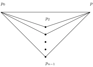
between the corresponding points is being queried. A prototypical 1-round algorithm uses
the line-rigid 3-cycle (or triangle) graph (Fig.1) as the core structure and constructs the
distance graph on n points.
that has edges joining the pairs of points whose distances are returned by the adversary. The
distances returned by the adversary are assumed to be valid if there exists a linear layout
consistent with these lengths. The distance graph is said to be line-rigid if a consistent layout
exists for all valid adversarial assignments of lengths. [21]
p0 p1
pn−1
p2
FIGURE 1: Distance graph for a 1-round algorithm
The best-known 2-rounds algorithm for point placement on a line is due to Alam and
Mukhopadhyay [3] that makes 9n/7 queries and has a query lower bound of 9n/8.
1.2
Point placement problem in 2D
The point placement problem on a plane is to determine the location of a linear set of points
{p1, p2, p3...pn} up to translation and reflection on the plane by making the fewest possible
pairwise distance queries to an adversary. This is a 2-dimensional version of Saxe’s problem.
In this thesis, we are proposing an algorithm for the point placement problem on a
plane based on Stochastic Proximity Embedding (SPE). A chordal graph is submitted to the
adversary as a distance query graph, while the remaining distances in the query graph are
uniquely determined using Stochastic Proximity Embedding (SPE). SPE also generates the
1.3
Point placement problem in 3D
The Molecular Distance Geometry Problem (MDGP) is defined as the problem of finding the
cartesian coordinates of the atoms in a molecule, with only a subset of pairwise interatomic
distances available. This is a 3-dimensional version of Saxe’s problem. The MDGP arises
in NMR experimental techniques that provides a set of inter-atomic distances dij for certain
pairs of atoms (i, j) of a given molecule.
The MDGP can be formulated as follows: A unique three-dimensional structure of a
molecule is to be determined when the distances between all pairs of atoms in a molecule are
available. However, when there are errors or unavailability of certain distances the unique
structure of the molecule may not exist. Here we are approaching the problem, with only a
partial set of interatomic distances available.
1.4
Motivation
The abstract version of point placement problem appears in diverse areas of research, such as
Wireless Sensor Networks (WSNs), Computational Geometry, Computational Biology and
Learning Theory [21].
Localization of sensor nodes has been an active research area in WSNs. Finding the
position of nodes is a vital requirement in many WSNs applications including tracking,
geometric routing, and monitoring [4]. Distances between the sensors are calculated by
measuring the power used between the sensors for two-way communications. Most of the
localization techniques are making use of the section of nodes that has prior knowledge of
their absolute positions. Such nodes are called anchor nodes. With the position of the anchor
nodes known, the localization problem is solved in the Wireless Sensor Networks (WSNs)
provided all other unknown distances are determined.
known as the turnpike problem. The problem description is as follows. In an expressway
from city A to city B, several ONroute exists; the distances between all pairs of ONroute are
known. With the know distances between the ONroutes, the geometric location of this route
is fixed. This problem was initially studied by Skiena et al. [27] who proposed a practical
heuristic for the reconstruction. A polynomial time algorithm was given by Daurat et al. [10].
In the area of Computational Biology, the 3D structure of a molecule can be determined
by solving the Molecular Distance Geometry Problem (MDGP) [9]. A molecule is represented
in a three-dimensional space by a set X. Each point xi in the set X is represents an atom
in the molecule. Some of the distances between atoms are determined by Nuclear Magnetic
Resonance (NMR) spectroscopy. By exploiting such distances, the coordinates of the atoms
in a molecule are determined by solving the corresponding Distance Geometry Problem. [13]
1.5
Preliminaries
Let D = [dij] be a symmetric matrix of size n×n and d(pi, pj) be the Euclidean distance
between the pointspi andpj. The symmetric matrix is said to be Euclidean distance matrix
if the pointsp1, p2, ...pnlies in some k-dimensional Euclidean space such thatdij =d(pi, pj)2.
The diagonal entries in the matrix are zero and the off-diagonal entries are filled with
Eu-clidean distances [23].
Let G= (V, E) be agraph, where V is the set of vertices and E is the edges. G consists of a finite set of vertices {v1, v2, ...vn} and a set of edges {{vi, vj}, i6=j} joining some pairs
of vertices. A path in the G is a sequence of vertices vi, vi+1, . . . , vk, where {vj, vj+1} for
j =i, i+ 1, . . . , k−1, is an edge of G. A cycleis the closed path in the graph and the size is the number of edges in the path. A chord is an edge joining two non-consecutive vertices in
connecting two vertices vi and vj if there is a non-zero entry in the ith row and jth column
of the distance matrix. [23]
In a graph G, the neighbourhood of a vertex v are those vertices in G that are adjacent tov. If the neighbourhood N(v) of a vertex is clique then the particular vertex is said to be asimplicial vertex. Asimplicial ordering of the vertices of Gis a map α:V → {1,2, . . . , n}
such that vi is simplicial in the induced graph on the the vertex set {vi, vi+1, . . . , vn}. [23]
1.6
Stochastic Proximity Embedding (SPE)
Stochastic Proximity Embedding (SPE) is the main tool we are using here to solve the point
placement problem in 2-dimensional and 3-dimensional spaces.
SPE is a self-organizing algorithm that attempts to generate the Euclidean embedding
that best preserves the similarities from the original embedding. SPE starts with a random
initial configuration and refines it by iteratively selecting a random pair of points. This
refine-ment starts adjusting the coordinates so that their distances on the map match more closely
with their respective proximities. The adjustment is driven by the learning-rate parameter
λ that decreases during simulation to avoid the oscillatory behavior. The main advantage of SPE is SPE scales linearly with respect to sample size and can be applied to the huge
data sets unlike the well-known dimensionality reduction techniques like multidimensional
scaling(MDS) and nonlinear mapping(NLM). [1]
Converting distances to coordinates is the prevalent theme in Distance Geometry
prob-lem. The prototypical example of this problem comes from the field of cartography. Intercity
distances are given in the form of a matrix; the aim is to place the cities on a two-dimensional
map that reflects their true geographical coordinates. The main idea of this problem is to
arrange a set of objects in space to reproduce the observed distances between them.
shows the relationship between these objects. let Pr = p
1a, p2a, ...pna be the random initial
point set produced by SPE, and the D= [dij] is a distance matrix showing the relationship
between the random point set. The distance matrix R can either be a partial or complete
distance matrix. SPE can produce the final embedding even when the distance between the
points are not fully available.
Algorithm 1 SPE
Initialize the coordinates of Pr and select an initial learning rate λ
for (C cycles) do for (S steps) do
Select a pair of points,pa
i and paj, at random and compute their distance dij =||pai −paj||. if (dij 6=rij) then
pa
i ←pai +λ12 rij−dij
dij+ (p a
i −paj), 6= 0
pa
j ←paj +λ 1 2
rij−dij dij+ (p
a
j −pai), 6= 0 end if
Repeat Step 2 for a prescribed number of steps,S
Decrease the learning rateλ by prescribed decrement δλ
Repeat Steps 2-4 for a prescribed number of cycles,C
Stochastic Proximity Embedding has two cycles, the outer cycle is the learning cycle,
and the inner cycle picks up the points randomly from the set Pr and applies the
Newton-Raphson Root finding style of correction to the randomly picked points. SPE is controlled
by three parameters: number of steps S, the learning rate parameter λ (C Cycles) and the term . The learning rate parameterλ starts with 1 and decreases over time to a final value 0.
The decrement of the λvalue forces the update rule to take more or less the full Newton-Raphson steps at the initial cycles and control the magnitude of the updates for the better
embedding; this prevents the oscillation of the updating algorithm. The value is chosen to be the smaller value and add with dij to avoid the division by 0 if points i and j happen to
coincide.
S is the number of times a random point is selected from the point set Pr. The parameter C
and S are set so thatCS =o(n2), as the quadratic running times of similar algorithms based
on Multi-Dimensional Scaling (MDS), Principal Component Analysis (PCA). The algorithm
designers have empirically determined that the algorithm scale linearly with the number
of data points. To achieve a practically perfect embedding, it takes 10,000 total pairwise
refinements per data point.
The quality of the embedding is measured by the stress function, the stress function is
minimized with the course of the refinement:
S = Σi<j
(dij−rij)2 rij
Σi<jrij
1.7
Thesis Organization
This thesis is organized in the following manner, a small description of the content in four
chapters that makes up the thesis.
• Chapter 2 gives a brief review of the Point placement on a line problem and
dis-cusses the motivation to study the point placement in the plane problem. After the
introduction to Sensor Network Localization, ’Distance matrix completion approach’
is reviewed, and a detailed description of our algorithm using SPE is discussed. Our
modified version of SPE is discussed to overcome the embedding in highest
transla-tion that SPE faces during algorithm executransla-tion. At last in the experiments sectransla-tion,
the comparison between Distance Matrix Completion Approach Vs. SPE with Partial
matrix Vs. SPE with complete matrix is analyzed.
• Chapter 3 introduces the Molecular Distance Geometry Problem (MDGP) and our
al-gorithm using SPE and DMCA to solve the MDGP. This chapter discusses the artificial
approach to reconstruct the chain of a protein molecule with partial distances. Our
approach towards solving the MDGP using DMCA and SPE is explained in detail.
MD-Jeep software proposed by Lover et al. [19] is reviewed, and the comparison
re-sults between MD-Jeep and the DMCA + SPE Approach is also discussed in the
experimentation section.
• Chapter 4 summarizes the topics discussed in this thesis and suggests some open
CHAPTER 2
Point Placement Problem on a Plane
2.1
Introduction
The point placement problem on a plane is to determine the location of a linear set of points,
{p1, p2, p3...pn} on the plane by making the fewest possible pairwise distance queries to an
adversary. The placement is fixed up to translation and reflection.
The main motivation behind this problem is to fix the sensor network localization. Sensor
networks have some nodes with their distances known, and other nodes with the unknown
distances. Now the problem is to fix the whole system using the available distances between
the nodes and the fixed nodes called anchor nodes [5].
2.2
Motivation
The current approach to the point placement on a line needs testing a large number of
distance constraints; these constraints involve the edge lengths of a distance graph. If integer
coordinates are used; we can avoid this problem of rounding errors; however for the point
placement on a plane this problem is unavoidable even if the coordinates are integral. Thus
we are using a distance matrix completion approach to avoid the problem of testing distance
constraints.
avoid the layer graph construction approach used for the point placement problem on the
line. The layer graph concept used in the point placement on a line is discussed below,
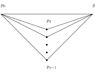
A prototypical 1-round algorithm constructs the following distance graph on n points (Fig. 2) by using the line-rigid 3-cycle graph or a triangle as a core structure. As the figure
shows that, the graph has n −2 triangles hanging from a common strut. The number of distance queries made is 2n−3
p0 p1
pn−1
p2
FIGURE 2: Distance graph for a 1-round algorithm
The distance graph can be re-drawn orthogonally, such re-drawn graph with satisfying
following conditions is called layer graph. The concept of layer graph is first introduced
by Chin et al. They also proved that a given distance query graph is not line-rigid iff it
has a layer graph drawing in [8]. Layer graph is also used to obtain the rigidity conditions.
Conditions to satisfy to be a layer graph:
1. All the edges in the graph Gshould be parallel to one of the two orthogonal directions
x and y
2. The length of an edgeeis the distance between the corresponding points on the distance
graph L
3. The edges in the graph should not be in a single direction
4. No two vertices coincide if the layer graph is folded onto a line, by a rotation either to
Mukhopadhyay et al. [21] showed that the rigidity conditions are easy to verify when exact
arithmetic is used in the implementation of the 2-rounds algorithm. Since the adversary is
simulated by us, the distances returned are set to be integral. There is a possibility of
rounding errors if the pairwise distances are not integral. Checking the rigidity conditions
can be difficult because of the rounding errors introduced in finite-precision calculations.
The approach proposed in this thesis is susceptible to generalization in higher dimensions,
where there are difficulties in generalizing the current approach to two or three dimensions
because of finding the suitable generalization of the layer graph concept and the theorems
associated with it.
2.3
Reductionist Approach
Though it is difficult to generalize the layer graph constructions in the point placement on
the line problem, reductionist approaches can be used to solve the point placement on a
plane problem by solving the point placement on the line problem. We discuss two such
reductions below,
Points on a two-dimensional integer grid
Consider the points p1, p2, p3, ...pn lie on an integer grid as shown in the figure below (Fig.
3). Now we can reduce the point placement on a plane problem to the point placement on
a line by projecting them on x and y axis. An important assumption is that no two points lie on the small vertical or horizontal line of the grid, to make sure that we have a distinct
p
1p
2p
3p
4p
5p
6x−axis y−axis
FIGURE 3: Points on a two-dimensional integer gird
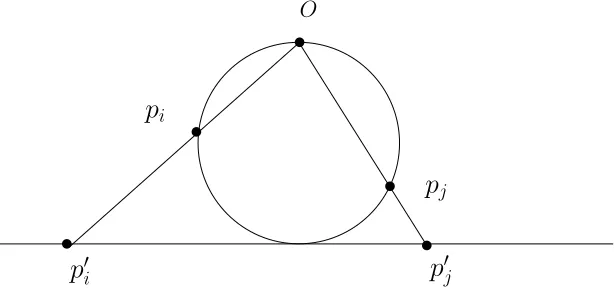
Stereographic projection of points on a circle
When points p1, p2, p3, ...pn lie on a circle, we can use stereographic projection on the circle
and plot the points on the line; now we can solve the problem by applying the 1-Dimensional
point placement algorithm to the projected points.
O
p
ip
jp
0ip
0jFIGURE 4: Stereographic projection of points on a circle
Stereographic projection is a mapping function that projects a sphere onto a plane. The
projection is defined on entire sphere except for one point where the projection is defined [29].
is the highest point in the sphere.
2.4
Prior Work
2.4.1
Sensor Network Localization Problem
Computing the locations of the nodes in a sensor network is known as the sensor network
localization problem. There are existing algorithms proposed to determine the location of
the nodes in a network by only knowing the location of fewer nodes. Such fixed nodes are
called beacon nodes. When the location of the fewer nodes are fixed, then other nodes try
to measure the distance between neighbors and fix their locations. Though algorithms exists
to find the location of the nodes, some fundamental questions were not addressed.
The theory of network localization proposed by Aspnes et al. [5] has some theoretical
proof to answer the basic questions in network localization. The main underlying idea in
this paper is this: grounded graphs are constructed to model the network localization and
the rigidity theory for graphs were used to test the conditions for unique localizability. Now
the unique networks were constructed using the rigid grounded graph.
The notion of grounded graphs is proposed in this paper [5] to solve the unique network
localizability. In grounded graphs, each vertex represents network nodes. If the distance
between two nodes is known, or the nodes are beacon nodes, then the corresponding vertices
are connected. With the construction of the grounded graphs, the network has a unique
localization if and only if its corresponding ground graph is generically globally rigid. To
check if a network in the plane is unique localizable, we just need to check if the corresponding
grounded graph is redundantly rigid and 3-connected.
The computational complexity of the network localization has been shown as NP-hard
when the grounded graph is generically globally rigid via reduction from set-partition.
localization. Aspens et al. [5] showed that the trilateration graphs are uniquely localizable
and the node locations are easily be computed. Aspens et al. also showed that the random
geometric graphs are trilateration graphs if a node density or the communication radius is
reached.
2.4.2
Distance Matrix Completion Approach
A distance matrix completion approach is proposed by Zamilur et al. [23] based on the
result of Bakonyi and Johnson. This approach includes the generation of a chordal graph,
computing simplicial ordering of the graph, finding the maximal clique and the distance
matrix completion. Once the distance matrix is completed the end coordinates are generated
by using the traditional Young and Householder’s method.
Computing a chordal graph sequence
Based on the result produced by Grone et al. in [14], chordal graph sequence is generated
in this paper. The theorem is as follows,
Theorem 1 [14] G has no minimal cycles of length exactly 4 if and only if the following holds: For any pair of vertices u and v with u 6=v, {u, v} ∈/ E, the graph G+{u, v} has a unique maximal clique which contains both u and v. (That is: if C and C0 are both cliques
in G+{u, v} which contain u and v, then so is C∪C0.)
Simplicial ordering computation
The simplicial ordering of a graph, αof G can be found by a breadth-first search of G when the vertices are labeled in the lexicographic order. A well-known LEX-BFS [24] algorithm is
Algorithm 2 Simplicial Ordering
1: Empty label list, (), is assigned to all the vertex in V
2: for i=n to 1 do
3: Pick a vertex v ∈V with the largest label list in lexicographical order
4: Set α(v) =i
5: For each unnumbered vertex w adjacent to v, add i to the label list ofw 6: end for
7: return α
Consider the following chordal graph for the simplicial ordering (Fig. 5) The vertices in
the chordal graph are labeled in lexicographical order.
FIGURE 5: A chordal graph on five vertices
By following the algorithm above, the simplicial ordering of the chordal graph is computed
and shown in the table below,
u v w x y
Step 0 () () () () ()
Step 1 () (5) (5) () ()
Step 2 () (5) (5,4) (4) (4)
Step 3 () (5) (5,4) (4) (4,3)
Distance matrix completion of a clique
To find a maximal clique, the algorithm designer is starting with a clique that has two
vertices of the given edge, add a vertex to the clique by examining if it is adjacent to every
other vertex in the clique; otherwise, discard the current vertex and move on to the next.
Distance matrix completion approach starts with the completion of a clique with one
edge missing in [23]; this theorem is formulated as the partial distance matrix completion
with one missing entry. The lemma proposed is as follows,
Theorem 2 This theorem is based on Bakonyi and Johnson’s results in [6]
The partial distance matrix admits at least one completion to a distance matrix F.
0 D12 x
Dt
12 D22 D23
x Dt 23 0
If
0 D12
Dt 12 D22
and
D22 D23
Dt 23 0
has embedding dimensions as p and q respectively then x can be chosen so that the em-bedding dimension of F is s=max{p,q}.
0 1 1 et 1
1 0 d12 D13 d14
1 d12 0 D23 x
e Dt13 Dt23 D33 D34
1 d14 x D
t 34 0
to a matrix in which the Schur complement
a B x−d12−d14
Bt C D
x−d12−d14 Dt f
of the upper left 2×2 principal matrix has a positive semidefinite completion of rank s.
0 1 1 0
Theorem 3 shows that the solution for x exists. [12] Let R =
a B x Bt C D
x Dt f
is a real partial positive semidefinite matrix. The rank of
a B Bt C
=p and rank of
C D Dt f
=q
Now the real positive semidefinite completion F of R shows that the rank of F is a
maximum of {p, q}. The completion shown here is unique iff rankC = p or rankC =q. Once the distance matrix is completed using the distance matrix completion approach,
the completed distance matrix is used as an input to the SPE and compute the coordinates.
To compare our results, coordinates are also computed using the Young and Householder’s
2.5
SPE Approach for Distance matrix completion
The distance query graph presented to the adversary is chordal. Once the chordal graph
is computed after the edge lengths returned by the adversary, the remaining distances are
uniquely determined using both the distance matrix completion approach proposed by
Za-milur et al. [23] and the Stochastic Proximity Embedding (SPE) heuristic. The coordinates
out of the completed distance matrix are computed using SPE.
Stochastic proximity embedding takesR= [rij] as a input distance matrix. The R matrix
can either be complete or partial distance matrix. In the next step, SPE produces a random
number of points equal to the size of the original embedding and computes the distance
matrix D= [dij].
Now SPE starts refining the point by iteratively selecting a random pair; the refinement
starts adjusting the coordinates based on the Newton-Raphson method of root-finding so
that their respective distances match closely. This adjustment is driven by the learning
rate parameter that decreases during simulation to avoid the oscillatory behavior. In our
approach, we kept= 0.0001, and the learning rate parameter goes from 1 to 0 decrementing by 0.001.
Algorithm 3 SPE
R= [rij] as a input distance matrix, select an initial learning rate λ
for (C cycles) do for (S steps) do
Select a pair of points,pa
i and paj, at random and compute their distance dij =||pai −paj||. if (dij 6=rij) then
pa
i ←pai +λ12 rij−dij
dij+ (p a
i −paj), 6= 0
pa
j ←paj +λ 1 2
rij−dij dij+ (p
a
j −pai), 6= 0 end if
Repeat Step 2 for a prescribed number of steps,S
Decrease the learning rateλ by prescribed decrement δλ
Repeat Steps 2-4 for a prescribed number of cycles,C
refined towards the original distance matrix R; the respective initial random points are also
refined towards the original embedding; thus these points are the final coordinates produced
by SPE.
While generating the coordinates using SPE, the values of the coordinates are translated
to the highest position. We used the geometric transformation to bring back the layout
close to the original layout without altering the structure of the layout. The Geometric
transformation is carried out using the Kabsch method.
The summary of the approach used in this problem is this; we are using the using the
distance matrix completion approach proposed by Zamilur et al. [23], based on the result
produced by Bakonyi et al. [6]. Bakonyi and Johnson showed that if the distance graph
corresponding to a partial distance matrix is chordal, then there exists a completion of
the partial distance matrix. Once the distance matrix is completed, we are computing
the coordinates using SPE. In the original method of completing the graph using Distance
matrix completion approach based on a result by Bakonyi and Johnson, coordinates are
generated using the traditional Young and Householder’s method [30]. We also approached
this problem by skipping the DMCA and input the partial distance matrix into SPE. The
result of both SPE with partial distance matrix and the SPE with complete distance matrix
and Young and Householder’s method is compared at the end of this problem.
The main difficulty we faced while generating the coordinates using SPE is that the
coordinates are transferred to the highest position. We discussed this problem further in
this thesis and proposed the solution to overcome this problem.
2.6
Difficulties in SPE
In SPE, the improvisation of the final embedding depends upon the parameters used inside
and improves the points embedding. The decrement we are using here for the λ affects the learning cycle. Some pointsets are tending to learn quickly, and the other needs more steps
to learn the original point positions. We have tested ourλ decrement from 0.01 to 0.5. The point set with more number of points and huge disparity over the original embedding took
more time to learn. While a point set with less number of points and less disparity with the
original embedding learned quickly and needed very few steps over λ.
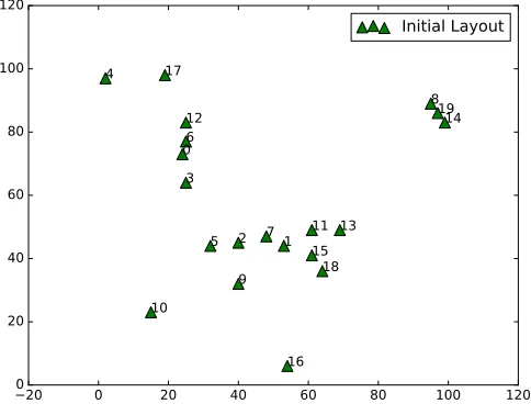
So what happens when the learning cycle is more for a point set that learns quickly. This
will overfeed the point set and translate the final structure to highest range. An example
showed here will give us the clear picture of what translation and overfeeding do to the point
set (See Fig: 7).
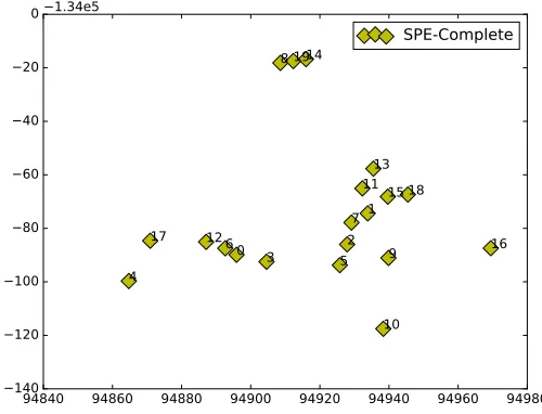
The figure below (Fig.7) shows the layout produced by SPE, which represents the original
layout (Fig.6) but in the highest range. The structure produced by SPE is same as the
original embedding (Needs Rotation), but the range in which SPE produced the embedding
is from 94980 to -1.35e5. The original embedding lies in the range of 120×120. This is the
result of the more number of learning cycles.
20 0 20 40 60 80 100 120 0
20 40 60 80 100 120
0
1 2 3 4
5 6
7
8
9 10
11 12
13
14
15
16 17
18
19
Initial Layout
94840 94860 94880 94900 94920 94940 94960 94980 140
120 100 80 60 40 20
0 1.34e5
0
1 2 3
4 5
6
7 8
9
10 11
12
13 14
15
16 17
18
19 SPE-Complete
FIGURE 7: SPE Layout of 20 points with 0.01 as learning rate
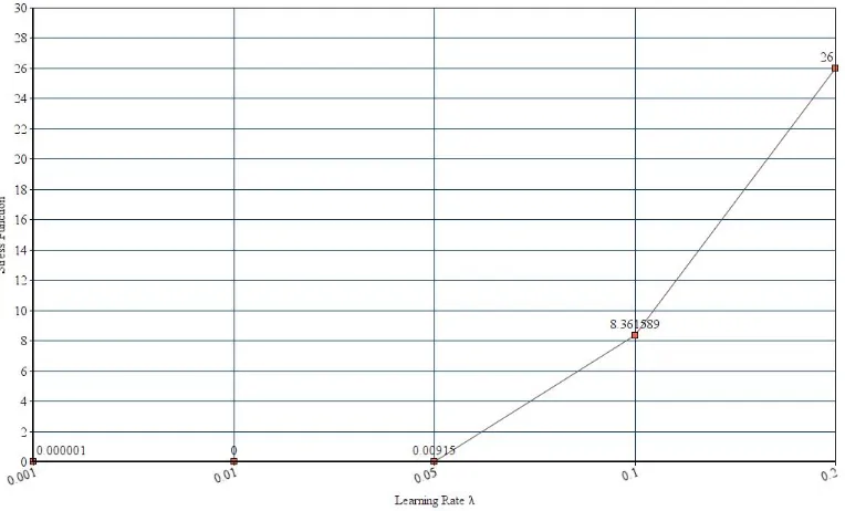
The experiment on the learning rate parameter is discussed here,
Through our series of experiments, we have got the clue that when the learning cycle is
more, then the stress function is close to zero. However, when this learning cycle overfeeds
the point set, then the translation to the highest position takes place. Below Few charts
(See Fig. 8 and 9) shows that the increase in learning cycles, steadily decreasing the stress
2.7
Modified Version of SPE
Since the learning rate parameter λ depends upon the number of points, and the disparity between the original and the approximate embedding, λ is hard to control. However, to control the highest translation of the point set, we have proposed the new idea of using anchor
nodes. Since the Sensor Network Localization has some nodes fixed, we are taking advantage
of such fixed nodes and fixing the remaining tag nodes without altering the positions of the
anchor nodes.
The updated SPE algorithm is as follows,
Algorithm 4 Modified SPE
Initialize the coordinates of Pr and select an initial learning rate λ
for (C cycles) do for (S steps) do
Select a pair of points,pa
i and paj, at random and compute their distance dij =||pai −paj||. if (dij 6=rij) then
if pa
i is Anchornode butpaj is notthen
pa
j ←paj +λ 1 2
rij−dij dij+ (p
a
j −pai), 6= 0 end if
if pa
i is not an Anchornode butpaj is an anchornode then
pa
i ←pai +λ12 rij−dij
dij+ (p a
i −paj), 6= 0 end if
if Both pa
i and paj is not an Anchor node then
pa
i ←pai +λ12 rij−dij
dij+ (p a
i −paj), 6= 0
pa
j ←paj +λ 1 2
rij−dij dij+ (p
a
j −pai), 6= 0 end if
end if
Repeat Step 2 for a prescribed number of steps,S
Decrease the learning rateλ by prescribed decrement δλ
Repeat Steps 2-4 for a prescribed number of cycles,C
Here we are choosing some points as Anchor points and running against the SPE
algo-rithm. Now in SPE, while choosing the i and j at random, we are not updating the anchor
and the other one as the tag node, then we are only updating the tag node.
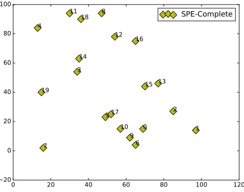
The figure (Fig. 11) shows the embedding of 20 points with λ = 0.001, for 20 points. This embedding is reproduced by SPE with learning rate parameter λ= 0.001 and keeping 2,4,6 as the anchor nodes, for 20 points the learning cycle that goes from 1 to 0.001 is more
than what is required. Since we can complete the 20 point structure with the learning rate
parameter λ= 0.01 (Fig. 7) but that translates it to the highest range.
The figure (Fig. 11) shows the SPE embedding with the range same as the original
embedding shown above (Fig. 10).
0 20 40 60 80 100 120 20
0 20 40 60 80 100
0 1
2 3
4
5
6 7
8
9 10 11
12
13 14
15 16
17 18
19
Initial Layout
0 20 40 60 80 100 120 20
0 20 40 60 80 100
0 1
2 3
4
5
6 7
8
9 10 11
12
13 14
15 16
17 18
19
SPE-Complete
2.8
Comparison and Experiments: DMCA (YH’s) Vs.
SPE Partial Vs. SPE Complete
The solution to the point placement problem is generated using three different methods
as discussed earlier. The first set of coordinates are computed by completing the distance
matrix using SPE. To compare our method, we have also computed the coordinates using
SPE heuristics and Young Householder’s method after completing the distance matrix using
distance matrix completion approach due to Zamilur et al. [23].
To match the layout more precisely we carried out the geometric transformation for each
method and calculated the error functions for both before and after geometric transformation.
Results produced by the experiments showed that the geometric transformation reduced the
error function for all three approaches. (See Table 1,2,3)
To measure the difference in the layout produced by three methods, we have computed
the RMSD value for the Young Householder’s method, SPE method and the SPE with partial
distance matrix method. We also calculated the localization error and the stress function for
both the SPE approaches. (See Table 1,2,3) All three methods are tested with the vertices
number ranging from 4 to 30.
Root Mean Square Deviation (RMSD) measures the difference between the original layout
and the computed layout. RMSD is calculated using the follwing formula,
RM SD(p, q) =
v u u t
1
n
n
X
i=1
((pix −qix)2+ (piy−qiy)2) (1)
where,
Stress function is proposed for SPE to measure the quality of the final layout with respect
the initial R matrix and the computed final D matrix. [2]
S = Σi<j
(dij−rij)2 rij
Σi<jrij
(2)
Localization error otherwise called as point placement error is similar to the RMSD error
calculation. Localization error measures the deviation between original point set and the
generated point set in the embedding. [4]
P P E(p, q) =
Pn
i=1((pix−qix)2+ (piy−qiy)2)
n (3)
In the figure (12,13,14,15) we displayed the embedding of the final coordinates between
all three methods. The embedding shown here is a perfect embedding with all three methods
are plotting the same layouts. The initial layout generated in this example is with 22 vertices
and 230 edges.
Vertices edges YH RMSD Before Rot YH RMSD After Rot and Trans
4 5 2061.38613755 332.718947801
5 9 2202.6379561 673.471908531
5 8 2184.59522219 424.666372119
5 7 2650.76500519 124.592855294
6 14 1721.47354557 978.613392827
6 13 2315.06013063 5.57342161115E-13
6 12 2347.68434379 4.81494292504E-13
6 11 2601.95709906 128.108823309
7 20 1412.12093121 2.97702022503E-13
7 19 2669.52612392 4.73031519081E-13
7 18 2093.8180598 1393.31680012
7 17 1960.70123927 4.28081464929E-13
7 16 2144.07021047 4.38731885205E-13
7 15 1790.96523847 4.09586882105E-13
7 14 3125.99749455 6.23799407748E-13
8 27 2120.4228321 5.61643470444E-13
8 26 2937.24305761 896.606749692
8 24 1879.95145333 6.16106521486E-13
8 23 2026.02999528 3.34710128792E-13
9 35 1974.59164777 3.70846133555E-13
10 44 3234.44076753 5.58397991437E-13
11 54 2608.67450477 4.89510925586E-13
11 53 3179.822133 5.36396664224E-13
11 52 3239.46433154 5.50984128278E-13
12 65 1889.3397251 8.78311012489E-13
12 64 1973.50863097 3.64950916711E-13
12 63 2995.28074733 1047.95976145
13 77 2005.28703062 5.3937923582E-13
13 76 2443.41425433 9.62375391148E-13
13 75 1855.65567995 1382.31670742
13 74 2883.51031415 5.48291421452E-13
14 90 1919.89125929 1336.18953834
15 104 3283.52995888 857.261738235
15 103 2230.62648667 5.88542166294E-13
17 135 2107.30234718 1172.11118029
17 134 2325.53513206 4.40644345245E-13
17 133 1766.74154046 5.58610690181E-13
18 152 1422.03923007 6.89913864166E-13
19 170 1992.917449 1176.21850955
19 169 1253.8446116 0.0000143580349942
20 189 2713.91084952 1.98613675909E-09
20 184 2002.66972301 1505.67912217
21 209 1255.39526647 9.06812995979E-13
21 208 3145.88993828 1.03290995258E-12
22 230 2339.99609327 4.07399115844E-13
22 228 1821.37130433 1347.60033124
23 252 1827.1580246 1225.90586641
23 251 2184.95489304 6.61271298836E-13
24 275 2639.50660174 1075.60235797
25 299 2778.85977602 6.80704391007E-13
25 298 1861.23667694 1149.65002139
26 324 2476.90641913 7.70174674996E-13
26 323 3345.33431099 1.04990677077E-12
28 377 2021.86398081 1102.61923649
29 405 2676.49811892 0.000000119304199898
30 434 2186.3878422 3.35898384949E-13
33 527 3202.94547 8.61732322337E-13
TABLE 1: Experimental results using Young Householders
Vertices edges RMSD Before Rot RMSD After Rot and Trans StressFunction LocalizationError
4 5 18043.260152 67.2144473019 1.07103318596E-27 4517.78192609
5 9 117260452730 673.471904629 2.84983750253E-22 453564.406325
5 8 30401178927.5 0.00000370931260326 1.01424435643E-23 1.37589999887E-11
5 7 1230539981.32 124.592849684 9.49870959458E-24 15523.3781925
6 14 41750608.783 3.22401107721E-09 6.96968329184E-30 1.0394247426E-17
6 13 1880142605.42 0.000000252528984187 3.26540827395E-26 6.37708878544E-14
6 12 1423401766.2 0.000000137402902514 2.64089262974E-26 1.88795576193E-14
6 11 107474288.164 878.660965831 1.58628969938E-25 772045.092875
7 20 1253520759.85 0.000000127021714005 1.07370474862E-26 1.61345158287E-14
7 19 76032392.5475 6.65464511504E-09 2.57579499774E-28 4.42843016072E-17
7 18 8494026.95063 7.50369912643E-10 8.54721111598E-32 5.630550058E-19
7 17 324900589.069 2.66470171063E-08 9.65131375856E-28 7.10063520663E-16
7 16 1220199.0529 1.11842189295E-10 8.32146480343E-32 1.25086753062E-20
7 15 2016199056.8 0.000000249663404461 6.8084183608E-27 6.2331815527E-14
7 14 654977701.028 3.58895384598E-08 1.72752560113E-27 1.28805897086E-15
8 27 12203416.2153 1.12849172436E-09 7.95728107259E-31 1.27349357196E-18
8 26 794572.013269 8.39558702951E-11 1.64224128046E-32 7.04858815701E-21
8 25 2357052.27682 3.70809939166E-10 4.40815551039E-32 1.37500010985E-19
8 24 34043351824.5 0.00000346269968413 1.7891785023E-23 1.19902891025E-11
8 23 93009999.5542 8.12612467333E-09 1.63753302522E-28 6.60339022066E-17
9 35 71155828.5831 4.38971193676E-09 1.00841270257E-28 1.92695708877E-17
10 44 4229986.82734 4.50251440449E-10 2.88406102408E-31 2.02726359626E-19
11 54 1799657.80778 2.08211736013E-10 1.48427659001E-31 4.33521270135E-20
11 53 422169.060493 6.28122502494E-11 9.77056323021E-33 3.9453787814E-21
11 52 3586209.66932 3.70071972899E-10 2.57635145283E-31 1.36953265125E-19
12 65 3132707.81416 2.49125816766E-10 8.06741997844E-32 6.20636725792E-20
12 64 2108317.3026 4.88032892833E-10 4.80715744332E-31 2.38176104487E-19
12 63 1087075.44575 0.000000353280421341 6.85180608122E-25 1.24807056103E-13
13 77 1960694.58685 4.28761937495E-10 1960694.58685 1.83836799044E-19
13 75 12851169.2444 1.67074435056E-09 2.54649749333E-30 2.79138668493E-18
13 74 48811374.0649 5.58594692648E-09 3.25228216205E-29 3.12028030654E-17
14 90 110840111.478 1336.18953834 1.28168087245E-28 1785402.48236
15 104 4971815.15998 0.000000095807194256 5.65828771036E-27 9.1790184712E-15
15 103 19082002.0952 1.79471706942E-09 3.66420584578E-30 3.22100935925E-18
17 135 1172.11118029 4.86786055487E-11 9.59141279618E-33 2.36960663817E-21
17 134 1239407.41191 1.57878955627E-08 2.69477369691E-28 2.49257646298E-16
17 133 81216598.0597 1.81133827455E-08 7.34479015195E-29 3.28094634486E-16
18 152 108727967.413 108727967.413 0.0000300756802658 46883.853731
19 170 3593977.78682 1.11830982222E-09 1.57337137176E-30 1.25061685847E-18
19 169 37337749.6678 22.4756510155 2.59568875049E-10 505.154888569
20 189 543818.408049 0.000000014400899914 2.47248417024E-27 2.07385918334E-16
20 184 43503204.2272 7.53211266093E-09 9.85438981199E-29 5.6732721137E-17
21 209 765367.835956 683.145241831 0.0007499345183 466687.421436
21 208 4259591.90917 0.47317370069 2.23715854946E-13 0.223893351024
22 230 6026680.76882 0.00147281265794 2.27632990959E-18 0.00000216917712538
22 228 1476638.90224 1347.60033124 7.46458354085E-31 1816026.65275
23 252 13113616.0313 0.000325732698814 1.38788410398E-19 0.000000106101791077
23 251 27549165.3342 6.2121943512E-09 2.52765601352E-29 3.85913586571E-17
24 275 14815753.7909 34.8381020592 1.26328187054E-08 1213.69335509
25 299 185799.642173 0.00369625794304 1.04843704534E-17 0.0000136623227815
25 298 4692133.25034 0.0365003333586 9.39914937104E-16 0.00133227433529
26 324 6309108.56324 1.61851733105 5.24165726042E-12 2.6195983509
26 323 2318986.54327 0.000000969851631606 4.48374916545E-25 9.40612187329E-13
27 350 4009822.91794 4.08266753546 1.3308693632E-11 16.6681742051
28 377 2862562.13634 7.31706445571E-10 3.89183384839E-31 5.3539432249E-19
29 405 21081460.7683 1117.89427484 1.46550922029E-26 1249687.60973
30 434 9701412.68314 0.301698010098 7.3270234131E-14 0.0910216892974
33 527 103497964.83 13.7797668849 1.66105871749E-10 189.881975402
TABLE 2: Experimental results using SPE with Complete distance matrix
Vertices edges RMSD Before Rot RMSD After Rot and Trans StressFunction LocalizationError
4 5 151716561583 447.53971618 1.45940642725E-08 200291.797558
5 9 63082137493.9 218.182826821 9.86929916464E-08 47603.7459198
5 8 182076180.074 214.943162064 0.000000825996971301 46200.562918
5 7 1565701696.72 220.033728419 0.0000003495825959 48414.8416419
6 13 1990608368.62 713.2369954 0.000000702661662933 508707.011607
6 12 188053348561 903.473784069 0.00000255635079899 816264.878499
6 11 28078410400.1 1092.40333631 0.0000010595213126 1193345.04918
7 20 30011934.6184 318.688834035 0.00000246357429019 101562.572939
7 19 5661286554.02 428.021783801 2.53839638228E-08 183202.647408
7 18 15604812.3723 1392.37641491 4.76273182696E-09 1938712.08079
7 17 1972392.7611 198.050289033 0.000000969798180351 39223.9169859
7 16 181668386.057 965.932099529 0.00000543690190933 933024.820901
7 15 4567403.53195 1344.50969055 2.66752040989E-08 1807706.30799
7 14 48902694.292 1366.51651125 0.00000036027510582 1867367.37553
8 27 3399860.58067 1053.12349407 0.000000028757641283 1109069.09376
8 26 237629108670 444.510525774 7.07463431011E-08 197589.607524
8 25 10151433.3375 1277.71324699 0.000000040292921175 1632551.14154
8 24 18570360.9301 1034.88711306 0.00000175796309786 1070991.33677
8 23 6894762.42834 868.401794764 0.0000236895672642 754121.677149
9 35 89657071.2847 510.622146958 9.89879381772E-09 260734.976964
10 44 5239487.51836 8.2381606773 2.09504908209E-10 67.867291345
11 54 15823092.5722 43.7650979351 1.60225150191E-08 1915.38379727
11 53 14533318.5163 265.699905269 4.70144893691E-08 70596.4396599
11 52 2040373.3106 738.603366932 0.00000244318789575 545534.933643
12 65 523602.748023 1117.1672964 1.33170679218E-09 1248062.76815
12 64 3925140153.81 762.178935519 0.0000131058237785 580916.729749
12 63 799995057.166 1085.62835938 3.11404774542E-08 1178588.9347
13 77 48552227.0725 1048.36217101 3.53973975995E-08 1099063.24161
13 76 27718246.2301 1296.47751865 6.81733894244E-08 1680853.95637
13 75 4255397.55139 248.781245178 0.00000510377354543 61892.1079521
13 74 984654.936116 234.080352689 0.000000731958485155 54793.6115149999
14 90 27809990.0635 16.4468275582 8.0732739609E-10 270.498136731
15 104 4543765.12073 172.855176775 0.000000110988511949 29878.9121379
15 103 1408879155.63 1074.39618261 0.000000809554377008 1154327.15722
17 135 17942836.1809 1.82901048341 1.89048375528E-11 3.34527934843
17 134 12984840.0703 33.738980696 4.90122953996E-09 1138.3188184
17 133 24230435.7011 1250.06200449 0.0000357565881358 1562655.01506
18 152 2560648736.25 455.200692716 0.000000274889950081 207207.67065
19 170 3667301.99917 39.1907401583 6.28887091454E-09 1535.91411415
19 169 611245.401946 95.7337519462 3.49251932534E-08 9164.95126169
20 184 11246377.5751 98.5656322344 2.97676589802E-08 9715.18385777
21 209 7882585.64085 5.96272819745 1.04865425194E-09 35.5541275567
21 208 1199791.95927 1153.01709326 2.69750872567E-08 1329448.41735
22 230 46268545.4521 0.74031023198 1.25198589858E-12 0.548059239574
22 228 11912594.9573 40.0911446337 1.64296544414E-08 1607.29987804
23 252 10347392.1173 1226.77007179 3.17758913889E-09 1504964.80904
23 251 29324633.4087 48.6902930533 1.10036558529E-08 2370.74463762
24 275 2422208.71519 40.382669602 0.000000030204515818 1630.76000418
25 299 83703247.2669 28.5757352436 1.73490847501E-09 816.572644712
25 298 4992171.22977 76.7177559965 0.000000025162310443 5885.61408514
26 324 418200163.297 10.0017692178 1.11647614028E-09 100.035387487
26 323 2391878098.21 74.1028457574 2.85547736168E-08 5491.23174934
27 350 21718647.8309 1271.83305156 2.60341881589E-09 1617559.31104
28 377 2666430.00197 47.2384964679 5.05523225628E-09 2231.47554855
29 405 1998787.8662 6.52573408417 2.99165833797E-10 42.5852053373
30 434 132581685.649 1222.62243382 0.0000273945141536 1494805.61567
33 527 472414526.944 20.9523650525 2.45922847911E-09 439.001601294
TABLE 3: Experimental results using SPE with Partial distance matrix
To compare the layouts created by three approaches, we have plotted the layouts to check
0 500 1000 1500 2000 2500 500 0 500 1000 1500 2000 2500 3000 0 1 2 3 4 5 6 7 8
9 10 11
12 13 14 15 16 17 18 19 20 21
FIGURE 12: Initial Layout with 22 Vertices
1500 1000 500 0 500 1000 1500 1500 1000 500 0 500 1000 1500 0 1 2 3 4 5 6 7 8 9 10 11 12 13 14 15 16 17 18 19 20 21 0 1 2 3 4 5 6 7 8 9 10 11 12 13 14 15 16 17 18 19 20 21 Initial Layout SPE-Complete
1500 1000 500 0 500 1000 1500 1500 1000 500 0 500 1000 1500 0 1 2 3 4 5 6 7 8 9 10 11 12 13 14 15 16 17 18 19 20 21 0 1 2 3 4 5 6 7 8 9 10 11 12 13 14 15 16 17 18 19 20 21 Initial Layout SPE-Partial
FIGURE 14: Initial Layout Versus SPE (Partial distance matrix)
1500 1000 500 0 500 1000 1500 1500 1000 500 0 500 1000 1500 0 1 2 3 4 5 6 7 8 9 10 11 12 13 14 15 16 17 18 19 20 21 0 1 2 3 4 5 6 7 8 9 10 11 12 13 14 15 16 17 18 19 20 21 Initial Layout Young-Householder
FIGURE 15: Initial Layout Versus Young and Householder’s approach
2.9
Discussions
Point placement on a plane has thrown up many open problems. While we used chordal
graphs in our approach, the extension to other classes of the graph remain open.
1500 1000 500 0 500 1000 1500 1500 1000 500 0 500 1000 1500 0 1 2 3 4 5 6 7 8 9 10 11 12 13 14 15 16 17 18 19 20 21 0 1 2 3 4 5 6 7 8 9 10 11 12 13 14 15 16 17 18 19 20 21 0 1 2 3 4 5 6 7 8 9 10 11 12 13 14 15 16 17 18 19 20 21 0 1 2 3 4 5 6 7 8 9 10 11 12 13 14 15 16 17 18 19 20 21 Init. Lay. YH SPE-C SPE-P
FIGURE 16: Initial Layout Vs Young and Householder’s approach Vs SPE(Partial matrix) Vs SPE(Complete matrix)
is plenty of potential in Stochastic Proximity Embedding, to explore the point placement
problems. The theoretical proof of SPE is still not clear and produces different results time
to time. In SPE, the learning rate parameter can be controlled with respect to the number
CHAPTER 3
Point Placement problem in 3D
Space with Degree of Freedom
Approach
3.1
Molecular Distance Geometry Problem
The Molecular Distance Geometry Problem (MDGP) is defined as the problem of finding
cartesian coordinates x1...xN ∈R3 of the atoms with only a subset of interatomic distances,
such that
||xi−xj||=d(i, j); ([i, j]∈S) (1)
In equation (1) S is the set of pairs of atoms [i,j] whose Euclidean distancesd(i, j) between
all the points are known. The problem can be solved in linear time if the distance between
all the pair of points is available [7, 11].
The distances are obtained through the NMR experiments or can be produced with our
knowledge of bond lengths and bond angles. If all the distances are given, then the problem
the eigenvectors to find the coordinates of the points if the distances are consistent and if we
can find the three non-zero eigenvalues of the matrix [9]. Also, to get the 3D coordinates,
the rank of the distance matrix should be less than or equal to three.
In practice, we cannot usually get the exact distances between all pairs of atoms in the
protein. Even NMR experiments can detect only the short-range distances between atoms
that are close to protein backbones. Saxe [25] showed that the problem is NP-hard when
the exact distances between the pair of points are not known [25]. EMBED algorithm from
Crippen and Havel is proposed to solve this problem by estimating the missing distances to
build the full set of distances. By estimating the remaining distances, we can now solve the
problem with the singular value decomposition [9].
The main motivation behind studying this problem is to determine the structure of the
protein molecules. Since NMR experiments can detect the short-range distances between
atoms of a protein molecule, we are computing the structure of the whole protein molecule
using only the distance between few pairs. Determined structure of a protein molecule will
give us a clue about its functionalities.
Determination of the three-dimensional structure of a molecule using a set of distances
between pairs of atoms is the goal of the Molecular Distance Geometry Problem (MDGP).
To test the algorithms designed to solve MDGP, we have created the artificial backbone
chain of a protein molecule using Philips model [17].
3.2
Prior Work
Molecular Distance Geometry Problem (MDGP) has been extensively studied and solved
in different forms [26]. More and Wu proposed a continuous approach to solve the MDGP.
The discretizable version of the same problem is proposed by Lover et al. [16] is called the
3.2.1
More and Wu’s approach
Different approaches have been proposed to solve the Molecular Distance Geometry
Prob-lem. More and Wu formulated the DGP as a continuous global optimization probProb-lem. The
problem is to find the position of the atoms in a molecule with only the distancedi,j between
some pairs (i, j) of atoms in a set S of the atom pairs. [18]
||xi−xj||=d(i, j); ([i, j]∈S) (2)
The set of constraints in the equation (2) is replaced by the penalty function. The
penalty function calculates the disparity between the computed and the known distances.
The penalty function is calculated using different approaches, one common method to
calu-culate the penalty function is the Largest Distance Error (LDE): [19]
LDE({x1, x2, ...xxn}) =
1
m
X
{u,v}
|||xu−xv|| −duv|
duv
(3)
m is the number of known distances.
In More and Wu’s approach, the global continuation approach is used to determine the
global solution to this problem. The continuation approach is shown to find the global
solution irrespective of the starting position.
3.2.2
Discretizable Distance Geometry Problem
The DMDGP is inspired by the protein molecules; protein molecules are formed by amino
acids and bound together forming a sort of chain. The atoms in the protein backbones which
are close in a sequence are also close in the 3D conformation of the protein structure. Since
NMR techniques can detect the short-range distances between the atoms, such distances are
To qualify as the DMDGP, the following assumptions needs to be satisfied,
Let G = (V, E, d) be a weighted undirected graph, with total order relation on the vertices. The two important assumptions are,
• Each quadruplet of E is a clique of consecutive vertices
• Triangle inequality must hold between every three vertices
When these assumptions satisfy, there are at least three lower level atoms connected to
the current atom. The intersection of this three points can either be a circle, two points or
only one point. With the triangle inequality in place, the intersection of three points cannot
be a circle. Because the three points cannot be aligned by satisfying the triangle inequality.
Since the intersection of three points is rarely one point only, they have taken two possible
positions for every atom.
Now with the two possible position, the binary tree is constructed. For every iteration,
two new positions are added to the binary tree after passing the feasibility test. Feasibility
test is just to test the agreement of the two possible position with the other available distances
if any such distance available other than the three distance used to compute the two possible
position. When a possible position is not agreeing with the other available distances, then
that branch is pruned out of the tree. This pruning phase reduces the binary tree quickly, and
the remaining branch is explored through an exhaustive search, which is not too expensive.
[19]
3.2.3
Crippen and Havel’s Approach
Crippen and Havel [15], proposed a solid algorithm to solve the molecular distance geometry
problem using the upper and lower bounds of distances instead of exact distances.
In the first step of the algorithm the given distance bounds are converted to distance
and Havel has been used to convert the bounds to limits. The limits that are calculated using
Floyd’s algorithm should satisfy the triangle inequality. The limits that satisfy the triangle
inequality is termed as triangle inequality limits.
For given three points u,v,w the lower bounds and upper bounds are denoted like this,
lu,w, uu,v, uu,w, lvw
Geometric set of rules are used for the bound smoothing, the upper and lower bounds of
the three given points should satisfy the following geometric rules.
lu,w =max(lu,w, lu,v −uvw, lvw−uu,v) (4)
uu,w =min(uu,w, uu,v+uv,w) (5)
In the next step of the algorithm, the distance limits are converted into distances, this
process of converting limits to distances is called Metrization. In this process of metrization,
one random distance is selected between the upper and lower bound. Once the random
number is selected, the upper and lower limits been set to this number and recompute the
triangle inequality limits.
In the next step of the algorithm, the coordinates are computed using the series of steps,
• The distance for each point is calculated from the center of mass.
• Where dij is the distance between the points i,j
• In the metric matrix A, each elemnt aij is computed form the origin
• B matrix is calculated like this, B = W A W
• Gale and householder showed that if B matrix is semi defininte then the coordinate
matrix X is obtained like this, X =σ√L
• Where L2 = [λ
12, λ22, ...λr2,0, ...0]
3.2.4
Philips Model
Philips model of instance creation is based on the method proposed by Philips et al. [22].
Philips model considers a molecule as being the chain of N atoms with Cartesian coordinates
given by x1, ..., xN ∈R3.
θij
i j
k l
rij
FIGURE 17: Philips Model
For every pair of consecutive atoms i,j,k,l :
• ri,j be the bond length which is the Euclidean distance between them.
• θi,k be the bond angle corresponding to the relative position of the third atom with
respect to the line containing the previous two.
• ωi,l be the torsion angle between the normals through the planes determined by the
atoms i,j,kand j,k,l
In most conformation calculations, all bond lengths and bond angles are assumed to be
fixed at their equilibrium values r0
i,j and θ0i,j, with regarding this we can fix the first three
We can always fix the first atom at originx1 = (0,0,0), and the second atom is positioned
at the distance of r12 from origin, i.e. x2 = (−r12,0,0), and the third atom is fixed at
x3 = (r23cos(θ13)−r12, r23sin(θ13),0). With the torsion angle ω14 fourth atom in the chain
is determined. With both ω14 and ω25 the fifth atom in the chain is determined, by fixing
another torsion angle ω36 the sixth atom in the chain is determined.
In Philips model the bond length and bond angles are set torij = 1.526◦ andθij = 109.5◦
respectively. The three preferred torsion angles at 60◦,180◦ and 300◦ are also specified in
the Philips model. With these three parameters, torsion angle, bond length, and bond angle
we can generate the distance between pairs of atoms and obtain instances for the Molecular
Distance Geometry Problem.
The torsion angle values are seen as perturbations of the preferred torsion angle 60◦,180◦
and 300◦. Based on the model described in Philips, we are generating the torsion angle by
adding the random value from the set {ω+i:i=−15◦, ...,15◦} to the random value out of
the three preferred torsion angle.
We are generating the cartesian coordinates to define the set S in (1), (xn1, xn2, xn3) is
defined as the cartesian coordinates for each atom in the chain using the following matrices,
[22]
xn1
xn2
xn3
xn4
=B1B2...Bn
0 0 0 1
(n = 1,...,N),
The matrix to calculate the cartesian coordinates is proposed by Philips et al. [22]
B1 =
1 0 0 0
0 1 0 0
0 0 1 0
0 0 0 1
, B2 =
−1 0 0 −r12
0 1 0 0
0 0 −1 0
0 0 0 1
,
B3 =
−cosθ13 −sinθ13 0 −r23cosθ13
sinθ13 −cosθ13 0 r23sinθ13
0 0 1 0
0 0 0 1
Bi =
−cosθ(i−2)i −sinθ(i−2)i 0 −r(i−1)icosθ(i−2)i
sinθ(i−3)icosω(i−3)i −cosθ(i−2)icosω(i−3)i −sinω(i−3)ir(i−1)i sinθ(i−2)icosω(i−3)i
sinθ(i−2)isinω(i−3)i −cosθ(i−2)isinω(i−3)i cosω(i−3)ir((i−1)i) sinθ(i−2)isinω(i−3)i
0 0 0 1
Once the cartesian coordinates for all the atoms are determined, the set S is generated with the cutoff value d, which in terms fetching the atoms i,j if their distance is within the cutoff value d. Cutoff value selection is defined as,
S= [i, j] :||xi−xj|| ≤d
A sample molecular chain created by the Philips model is shown here, (Fig. 18)
3.3
Overview of our results
We proposed the Degree of freedom (DoF) approach to fetch the partial distances out of a
molecular chain and construct the whole chain of a molecule. For each atom, if the distance
by constructing the chordal graph with the partial distances. This gives us the freedom to
use DMCA due to Zamilur et al. and the SPE due to Agrafoitis to complete the remaining
distances and solve the Molecular Distance Geometry Problem (MDGP).
With the available distances, the partial distance matrix is computed and is completed
using both DMCA and SPE. One the distance matrix is completed then the coordinates are
generated using SPE.
We tested our DoF approach with the artificial instance created using the Philips model
and obtained good results out of it. In addition to the artificial instances, we have also
compared our approach with the Md-Jeep approach due to Carlie Lover et al. [19]. Synthetic
NMR datasets available with MD-Jeep are used while comparing the MD-Jeep with our DoF
approach.
7 6 5 4
3 2 1 0 1
1.0 0.5 0.0 0.5 1.0 1.5 2.0 2.5 1.2 1.0 0.8 0.6 0.4 0.2 0.0 0.2
0 1 2
3 4
5