University of Windsor University of Windsor
Scholarship at UWindsor
Scholarship at UWindsor
Electronic Theses and Dissertations Theses, Dissertations, and Major Papers
12-12-2018
Performance Evaluation of Competing Data Structures
Performance Evaluation of Competing Data Structures
Mohsen Tavakoli University of Windsor
Follow this and additional works at: https://scholar.uwindsor.ca/etd
Recommended Citation Recommended Citation
Tavakoli, Mohsen, "Performance Evaluation of Competing Data Structures" (2018). Electronic Theses and Dissertations. 7626.
https://scholar.uwindsor.ca/etd/7626
This online database contains the full-text of PhD dissertations and Masters’ theses of University of Windsor students from 1954 forward. These documents are made available for personal study and research purposes only, in accordance with the Canadian Copyright Act and the Creative Commons license—CC BY-NC-ND (Attribution, Non-Commercial, No Derivative Works). Under this license, works must always be attributed to the copyright holder (original author), cannot be used for any commercial purposes, and may not be altered. Any other use would require the permission of the copyright holder. Students may inquire about withdrawing their dissertation and/or thesis from this database. For additional inquiries, please contact the repository administrator via email
Performance Evaluation of Competing
Data Structures in Pathfinding
By
Mohsen Tavakoli
A Thesis
Submitted to the Faculty of Graduate Studies through the School of Computer Science in Partial Fulfillment of the Requirements for
the Degree of Master of Science at the University of Windsor
Windsor, Ontario, Canada
2018
c
Performance Evaluation of Competing Data Structures in Pathfinding
by
Mohsen Tavakoli
APPROVED BY:
M. Hlynka
Department of Mathematics and Statistics
M. Kargar
School of Computer Science
S. Goodwin, Advisor School of Computer Science
DECLARATION OF ORIGINALITY
I hereby certify that I am the sole author of this thesis and that no part of this
thesis has been published or submitted for publication.
I certify that, to the best of my knowledge, my thesis does not infringe upon
anyone’s copyright nor violate any proprietary rights and that any ideas, techniques,
quotations, or any other material from the work of other people included in my
thesis, published or otherwise, are fully acknowledged in accordance with the standard
referencing practices. Furthermore, to the extent that I have included copyrighted
material that surpasses the bounds of fair dealing within the meaning of the Canada
Copyright Act, I certify that I have obtained a written permission from the copyright
owner(s) to include such material(s) in my thesis and have included copies of such
copyright clearances to my appendix.
I declare that this is a true copy of my thesis, including any final revisions, as
approved by my thesis committee and the Graduate Studies office, and that this thesis
ABSTRACT
Pathfinding is an essential part of many applications, including video games and
robot navigation. A pathfinding algorithm usually finds a path from the given starting
point to the endpoint. Many different implementations of pathfinding solutions exist
in the industry. One of the most known and used of these algorithms is A*. A* will
find the shortest path from the starting point to the endpoint. Classic A* algorithm
can guarantee the shortest path to the desired destination which was introduced in
1968 by Hart, Nilsson, and Raphael. A* is widely used in the game industry to solve
the shortest path problem. The A* algorithm utilizes two data structures. A* explores
the nodes in the graph from the start position one by one and assign them a value
of F which is the sum of G cost and H cost. G Cost is the actual cost of exploring
the node from the starting position to the current node, andH cost is the estimation
of the cost of from the current node to the goal node. The Open List keeps all of
the nodes that are not explored at each iteration of the algorithm. In each iteration,
the algorithm removes the node with the least value ofF cost and run the algorithm.
If the node is not the goal, it will be added to the closed list. Interactions with the
open list, which are insert (current node) and remove Min, are costliest part of the
algorithm. It is well known that using a priority queue will increase the performance
of this algorithm. A number of priority queues have been used to implement A* and
improve the performance of this algorithm. We propose to use a Lazy binary heap
and evaluate its performance compare to other data structures. We expect that due
AKNOWLEDGEMENTS
I would like to express my sincere appreciation to my supervisor Dr. Goodwin
for being patient with me and helping me to come up with the idea of the Partial
Min-Heap. Thanks to his plenty of guidance and encouragement, I had a great time
to research the field of pathfinding. It is my great pleasure to be his student and
work with him.
I would also like to thank my committee members Dr. Kargar and Dr. Hlynka for
taking the time to review my paper and attending my thesis proposal and defense.
Thanks for their valuable guidance and suggestions to improve this thesis.
The time that I spent on this thesis has been very intense. To anyone reading this
paper, I will say that with hard work and commitment, you can achieve your goal in
life.
Finally, I would like to thank my parents, my dear brothers Ahmad and Ehsan
TABLE OF CONTENTS
DECLARATION OF ORIGINALITY III
ABSTRACT IV
AKNOWLEDGEMENTS V
LIST OF TABLES VIII
LIST OF FIGURES IX
1 Introduction 1
1.1 Thesis Claim . . . 1
1.2 Pathfinding . . . 1
1.2.1 Pathfinding Problem . . . 1
1.3 Graph Representations . . . 2
1.3.1 Waypoints . . . 2
1.3.2 Navigation Mesh . . . 2
1.3.3 Grids . . . 3
1.4 Heuristic . . . 4
1.4.1 Manhattan Distance . . . 5
1.4.2 Euclidean Distance . . . 5
1.5 Pathfinding Algorithms . . . 6
1.6 A* Algorithm . . . 7
1.6.1 Heuristic Consistency . . . 10
1.6.2 Problem Statement . . . 11
1.6.3 Min-Heap Example . . . 12
1.7 Thesis Contribution . . . 13
1.8 Thesis Organization . . . 14
2 Literature Review 16 2.1 A* Data Structure . . . 16
2.2 Closed Set . . . 17
2.3 Open Set . . . 17
2.3.1 Array . . . 18
2.3.2 Hash Table . . . 18
2.3.3 Binary Min-Heap . . . 19
2.3.4 Fibonacci Heap . . . 21
2.3.5 Multilevel Buckets . . . 22
2.3.6 MultiQueues . . . 22
2.3.7 Heap On Top Priority Queues . . . 23
3 Cached Min-Heap and Partial Min-heap 26
3.1 Motivation . . . 26
3.2 Cached Min-Heap . . . 29
3.2.1 Cached Min-Heap Operations . . . 30
3.3 Partial Min-Heap . . . 36
3.3.1 Partial Min-Heap Operations . . . 36
3.4 Partial Min-Heap Case study . . . 39
3.4.1 Partial Min-Heap Success . . . 39
3.4.2 Partial Min-Heap Failure or Sub-optimallity . . . 41
3.4.3 Summary . . . 41
4 Experiments and Results 42 4.1 Implementation Methods . . . 42
4.2 Experimental Environment . . . 43
4.3 Experiment Setups . . . 44
4.4 Performance Evaluation . . . 45
4.4.1 Success . . . 45
4.4.2 Time . . . 45
4.4.3 Path Length and Cost . . . 46
4.4.4 Nodes Expanded . . . 46
4.4.5 Operations . . . 46
4.5 Experiment Results and Analysis . . . 49
4.6 Number of operations . . . 51
4.7 Runtime . . . 62
4.8 Summary . . . 64
5 Conclusion 68
6 Future Work 70
APPENDICES 71
REFERENCES 87
LIST OF TABLES
1 Time Complexity Comparison of Different Data Structures . . . 24
2 Summary of experiments . . . 50
3 Map Size 120*120 using K=6 Full Data . . . 72
4 Map Size 120*120 using K=7 Full Data . . . 73
5 Map Size 120*120 using K=8 Full Data . . . 74
6 Map Size 200*200 using K=6 Full Data . . . 75
7 Map Size 200*200 using K=7 Full Data . . . 76
8 Map Size 200*200 using K=8 Full Data . . . 77
9 Map Size 200*200 using K=9 Full Data . . . 78
10 Map Size 300*300 using K=8 Full Data . . . 79
11 Map Size 300*300 using K=9 Full Data . . . 80
12 Map Size 400*400 using K=8 Full Data . . . 81
13 Map Size 400*400 using K=9 Full Data . . . 82
14 Map Size 400*400 using K=10 Full Data . . . 83
15 Map Size 512*512 using K=9 Full Data . . . 84
16 Map Size 512*512 using K=10 Full Data . . . 85
LIST OF FIGURES
1 Waypoint Map . . . 3
2 Navigation-Mesh Map . . . 3
3 Square-Grid Map . . . 4
4 Manhattan & Euclidean Distance . . . 6
5 A* algorithm on the left & Best-First search in the middle & Dijkstra’s algorithm on the right finding the same path . . . 8
6 Current Min-heap . . . 12
7 Problem Itteration 1 . . . 12
8 Current Min-heap . . . 13
9 Problem Itteration 2 . . . 13
10 Current Min-heap . . . 13
11 Problem Itteration 3 . . . 13
12 Implementation of Min-Heap using an Array . . . 19
13 Inserting to Min-Heap . . . 20
14 Remove Min - Min-Heap . . . 21
15 Fibonacci-Heap Insert Example . . . 22
16 Example of search environment . . . 27
17 Example of search environment (Exploring a node) . . . 27
18 Example of search environment (Exploring a node) . . . 28
19 Cached Min-Heap Data Structured=3 . . . 30
20 Cached Min-Heap Data Structure Exampled=3 . . . 31
21 Cached Min-Heap Data Structure Exampled=3 . . . 32
22 Cached Min-Heap Data Structure Exampled=3 . . . 32
25 Partial Min-Heap Data Structure Insert Example d=3 . . . 38
26 Partial Min-Heap Data Structure Remove Min Exampled=3 . . . 38
27 Pathfinding Example . . . 40
28 Pathfinding Example . . . 40
29 Pathfinding Example . . . 41
30 Map Size 45*45 - Obstacle chance 10% . . . 43
31 Map Size 60*60 - Obstacle chance 10% . . . 49
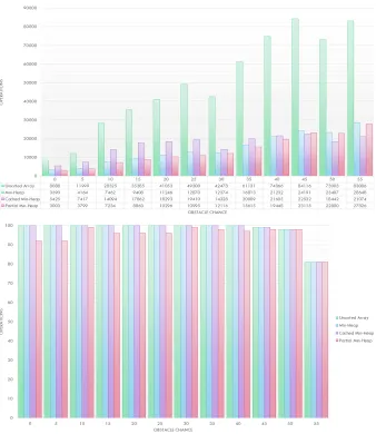
32 Map Size 120*120 using K=6 Full Data in Table 3 . . . 52
33 Map Size 120*120 using K=7 Full Data in Table 4 . . . 53
34 Map Size 120*120 using K=8 Full Data in Table 5 . . . 54
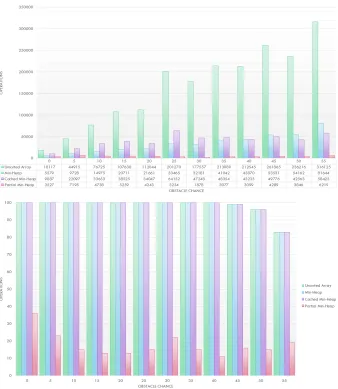
35 Map Size 200*200 using K=6 Full Data in Table 6 . . . 55
36 Map Size 200*200 using K=7 Full Data in Table 7 . . . 56
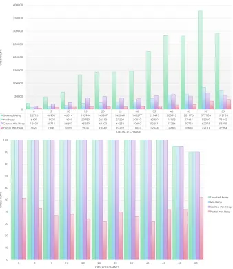
37 Map Size 200*200 using K=8 Full Data in Table 8 . . . 57
38 Map Size 200*200 using K=9 Full Data in Table 9 . . . 58
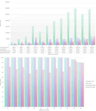
39 Map Size 300*300 using K = 8 Full Data in Table 10 . . . 59
40 Map Size 300*300 using K = 9 Full Data in Table 11 . . . 60
41 Map Size 400*400 using K=8 Full Data in Table 12 . . . 61
42 Map Size 400*400 using K=9 Full Data in Table 13 . . . 62
43 Map Size 400*400 using K=10 Full Data in Table 14 . . . 63
44 Map Size 512*512 using K=9 Full Data in Table 15 . . . 64
45 Map Size 512*512 using K = 10 Full Data in Table 15 . . . 65
46 Map Size 512*512 using K = 11 Full Data in Table 16 . . . 66
47 Run Time Map Size 400*400 using K=9 & 10 . . . 67
CHAPTER 1
Introduction
1.1
Thesis Claim
In this thesis, we present two new data structures for the A* search algorithm which
implement the open set Partial MinHeap, and Cached MinHeap. Test results in
comparison to traditional data structures used for this algorithm, such as unsorted
list, min-heap and heap-on-top priority queue (Hot Queue), show improvements in
runtime. Additionally, because of the distributed architecture of this data structure,
the number of operations is often reduced.
1.2
Pathfinding
Pathfinding is the task of finding a traversable path from the starting position to the
ending position. A universal problem which exists in multiple areas such as games,
robotics and computer networks. These problems require a reliable solution. In this
thesis, we focused on improving the A* algorithm performance in fully connected
grids.
1.2.1
Pathfinding Problem
1. INTRODUCTION
algorithm, A*, Hierarchical and Cooperative pathfinding algorithms. This research
aimed to find a better solution for A* Open set, which has a significant impact on
runtime. In this research, we treat operations and time as a performance variable.
We came up with a solution that delivers suboptimal path, using less memory and
time which could be a better solution in the right circumstances.
1.3
Graph Representations
In pathfinding, we need a representation of the search space for our algorithm to find
a correct path from our starting point to our ending point. A pathfinding algorithm
tries to find a path using a simplified representation of the search space. Common
ways of representing the maps are Waypoints, Navigation Meshes, and Grids.
1.3.1
Waypoints
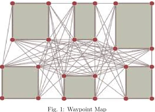
Using a collection of linked and fully connected nodes for navigation is the
way-point(Fig. 1) system. Each waypoint refers to a physical space or coordinates in
the map. AI agents are capable of traveling from one waypoint to another waypoint.
Game engines such as Unity3D, Unreal Engine support waypoints. The advantage
of using waypoints is that it will decrease the amount of memory usage since it uses
fewer nodes [13]. The disadvantage of waypoints is that the path found is unrealistic
and sub-optimal. Waypoints are usually created manually by the developer to have
the highest performance.
1.3.2
Navigation Mesh
Navigation meshes(Fig. 2) or nav-mesh are a way of representing the map with a
group of polygons connected within the map. Each polygon can have attributes such
as the cost of traversing, type of terrain, require a tool to pass, etc. We do not need
to store the obstacles in navigation mesh. Agents are free to roam from polygons to
1. INTRODUCTION
Fig. 1: Waypoint Map
reach the desired destination. Using polygons to represent nodes in the map results
in using less memory, but the path quality will suffer.
Fig. 2: Navigation-Mesh Map
1. INTRODUCTION
walkable or cost. Grids will cover all of the game maps such as obstacles. Nav-mesh
and waypoints only addressed areas that are traversable. Commonly used forms are
squares, triangles and hexagonal.
Fig. 3: Square-Grid Map
Square tiles are the most common grid(Fig. 3). Each tile in the map uses the
fa-miliar X, Y coordinates. Most of the commercial games such as Warcraft III, Dragon
Age: Origins are using grids in their games. Each grid has three different parts: tiles,
edges, and vertices. Faces are a 2D surface surrounded by the edges. Lines that are
enclosed by two vertices are edges. Each vertex is the point where each tile’s edges
meet to form the desired shape.
In this research, we ran experiments using squared grids since they are easy to
visualize and implement. We ran our tests on randomly generated maps with a chance
of blocking grid cells. Based on the suggestion [23] we ran our experiments using an
implementation of A* on fully connected squared grids so that other scientists can
compare their results to our results.
1.4
Heuristic
Classic search algorithms such as Dijkstra’s algorithm explore the search space to
find the shortest path. The heuristic function guides the algorithm into the direction
1. INTRODUCTION
faster[19]. The heuristic value is an estimation of the path cost from any given node
and represented as h(n). If our heuristic has a value of 0, our A* algorithm will act as
Dijkstra’s algorithm. If the returned value by our heuristic function is smaller or equal
than the actual cost of reaching the goal, A* is guaranteed to find the optimal path. If
the value is greater than the actual cost of the path, A* is not guaranteed to find the
optimal path. If our heuristic function is not admissible, which means that it will not
overestimate or underestimate the cost of the actual path, our pathfinding algorithm
is guaranteed to find the optimal path, which means that if our heuristic is accurate,
it will result in that our pathfinding algorithm only expanding the nodes along the
path. The developer can pre-compute the heuristic value the shortest path between
any pair of nodes in the map. This approach is not suitable for large maps since
that the precalculated heuristic values occupy more memory than the search space
representation [4]. There are three well-known heuristics functions for calculating the
shortest distance between two given nodes namely, Manhattan distance and Euclidean
distance.
1.4.1
Manhattan Distance
This heuristic is standard for squared grids that movement is only allowed
non-diagonally. Manhattan distance is not admissible since it overestimates the cost of
diagonal movements.
M anhattanDistance=|dX|+|dY| (1)
1.4.2
Euclidean Distance
Euclidean distance is the mathematically calculated straight-line distance between
1. INTRODUCTION
requires computational power, in some of the cases not using the heuristic function
might result in less number of operation to find the correct path [14].
EuclideanDistance=√dX2 +dY2 (2)
Fig. 4: Manhattan & Euclidean Distance
In our research, we designed our agent to be able to move in eight directions
and our map representation was squared grids. We used squared grids since that
it was easy to implement and understand. Also, most of the commercial games use
this representation, and we wanted to compare our results compare to actual game
maps. We selected our heuristic function as Euclidean distance based on our map
representation and our agent’s movements. We fixed our non-diagonal movement cost
to 10 and our diagonal movement to 14.
1.5
Pathfinding Algorithms
The single source shortest path problem is searching for a traversable path with the
least path cost from a given source to the desired destination. Existing solutions for
this problem divide to two categories: informed and un-informed search.
Breadth-first Search and Depth-Breadth-first search do not use the heuristic information available
based on the map, so their performance suffers since they blindly search for the goal
node. Not using the existing data will result in exploring multiple unnecessary nodes,
1. INTRODUCTION
of finding a solution to the shortest path problem is using the given information
to optimize the process of finding a solution. Information such as the location of
the goal node in the search space, the relative cost of reaching the goal node might
help our pathfinding algorithm to perform better in terms of the number of nodes
expanded. A* algorithm [15] and Dijkstra’s algorithm [9] are two of the most popular
solutions for solving this problem. Game industry mostly used A* to develop and
solve their pathfinding problems since it requires less computational power and it
has better performance compare to Dijkstra’s algorithm. Researchers and developers
proposed different versions of A* algorithm to increase the performance of it [4] and
mostly tailor it to their need. Researchers suggested that improvements are possible
in terms of performance by pre-calculating and processing of the map in Partial
Pathfinding[22] for A* algorithm. Algorithms such as Hierarchical Pathfinding A*
[3] proposed a clustering solution to divide the search space into local and global
clusters. Iterative Deepening A*[17] combined the depth-first search algorithm with
A* algorithm which uses the heuristic function to guide the search algorithm in the
correct path.
Our primary focus in this research paper is the widely explored and popular A*
pathfinding algorithm. We analyzed the performance of the A* algorithm’s data
structures and believed that we could improve its performance.
1.6
A* Algorithm
A combination of the Dijkstra’s algorithm and greedy Best First Search is A* search
algorithm. Dijkstra’s algorithm is guaranteed to find the shortest path, but it explores
all the directions in the search space and will allow us to find the path to multiple
locations. Best First Search explores in the goal direction to find the shortest path,
1. INTRODUCTION
Fig. 5: A* algorithm on the left & Best-First search in the middle & Dijkstra’s algorithm on the right finding the same path
node, to find the shortest path to the goal node. Best-First search uses f(n) = h(n),
which is the estimated cost from the current node to the goal node, to find the shortest
path. A* algorithm combines these two values to find the shortest path to the goal
node.
A* search algorithm constructs a path from the starting node to the goal node by
following the nodes with the lowest f cost. This algorithm keeps track of alternative
path nodes with their f cost. In each state, A* algorithm will expand the node with
least f value till it reaches the goal node.
A* algorithm maintains two data structures to function. A* keep the nodes that
have been visited but not expanded in theopenset. These nodes are a queue of nodes
that are possible to be the shortest path. Closedsetcontains already expanded nodes
that have been extracted from the openset and examined.
A* algorithm initially inserts the starting node into the openset. Then the
al-gorithm will explore all of the traversable neighbours of the current node with the
smallestf cost in theopenset, calculate theirf cost and insert them into theopenset.
Since it is required to keep track of each node’s path to the current location, each node
also holds a pointer to its parent. The algorithm chooses the node with the smallest
f cost from the openset. If the current node is not the goal node, the algorithm will
insert the node to the closed set, and it will repeat the process till that either to find
1. INTRODUCTION
path.
f(n) = g(n) +h(n) (3)
Calculating the current f cost of noden is the total ofg(n) and h(n). The actual
cost of reaching the node n from the starting node is g(n) and the estimated of cost
of reaching the goal node from the node n is h(n).
A* Algorithm.3 is fairly simple to implement and understand. Initially our open
setis empty, so we add thestartnode to the open setand calculate thef cost for the
start node. Our main loop, extract the current node with the least value of f cost
from the open set in each iteration and examine it. If the current extracted node is
our goal node, then the algorithm will return the path from the starting node to the
goal node. To find the path from the start node and to our goal node, each node
also keeps a pointer to its parent node. If the currentnode is not our goal node, the
algorithm will remove thecurrent node from the open set, insert it to theclosed set
and it will explore all of it’s neighbours. If the neighbour is not in our closed set,
and it is not a member of the open set, then the algorithm will insert it to theopen
setand set thecurrent node as the parent node for it. If the neighbour node already
exists in theopen setthe algorithm will calculate a newf cost for the neighbour node.
If the new f cost is greater equal to the current f cost, the node will be discarded.
Otherwise, the new f cost will replace the old f cost and set the current node as
the new parent for the neighbour node. The reason for this if statement is that we
do not want to insert duplicate nodes that have been already explored back into our
open set.
A* search algorithm is guaranteed to find a solution if there is one which means
that it is complete. Pathfinding solutions are exponential problems which means that
1. INTRODUCTION
Algorithm 1 A* Algorithm
1: Start:
2: open set = {start}
3: f(start) = h(start)
4: closed set = { }
5: while open set is not emptydo
6: current = extract the node with lowest f cost from open set
7: if current = goal nodethen
8: return “Path found”
9: end if
10: open set.remove(current)
11: closed set.insert(current)
12: for eachneighbour of current do
13: if neighbour in closed set then
14: continue
15: end if
16: if neighbour not in open list then
17: open set.insert(neighbour)
18: end if
19: if g(current) + distance(current, neighbour) < g(neighbour) then
20: g(neighbour) = g(current) + distance(current, neighbour)
21: f(neighbour) = g(neighbour) + heuristic f unction(neighbour, goal) 22: neighbour.setParent(current)
23: end if
24: end for 25: end while
26: return “Failed to Find the Path”
RTS games, as long as the path introduces to the agent is close enough to the actual
shortest path and it is not irrational in terms of movement, it is an acceptable path.
1.6.1
Heuristic Consistency
A* algorithm chose the best node to explore from the open set using the cost function
which is f(n) = g(n) + h(n) where g(n) is the actual distance or cost of travesing
to node n and h(n) is the estimated cost of reaching the goal node. If our heuristic
function is consistent the cost of traversing from our node x to the next node y will
be [15]:
1. INTRODUCTION
This means that by moving from x to y, our overall cost of reaching the goal cannot
be reduced more than the estimated cost of traversing from node x to the node y. If
the node that our agent is exploring is the neighbour of the node x, the value of f
is consistent since the g(n) will increase as much as the h(n) decreases[20]. We can
define our consistent heuristic as:
|h(x)−h(y)| ≤d(x, y) (5)
Based on those mentioned above, we can state that if our heuristic function is
consistent while exploring the neighbours of the node x, our neighbour’s f value
is equal or smaller to the current node’s f value. Using this information, already
explored nodes in the closed setwill not be revisited [16].
Theorem 1 A consitent heuristing will garantee a non-decreasing f value while
ex-ploring along the path.
Based on the Theorem 1, our A* algorithm will not revisit the nodes that are
already explored, and we can skip the nodes that are already explored once in
Algo-rithm 1 line number 16. Also, we can obtain that if our heuristic function is consistent
and admissible, our number of expanded nodes is optimal [15]. If our heuristic
func-tion is not consistent but admissible, nodes in the closed set can be revisited [18] to
find the path. Based on the theorem we can state that, if our heuristic is admissible
and consistent, the A* search algorithm only expand the nodes that their f value is
either smaller or equal to the current expanded node in theopen set.
1.6.2
Problem Statement
Majority of the computational power required to find a path in A* algorithm happens
1. INTRODUCTION
if our heuristic function is consitent[24]. The data structure of the open set is a
critical section of this problem, and it will help the algorithm to perform better or
worst based on the solution. One of the widely used solutions for this problem is the
binary Min-Heap. Heap data structure is sensitive to the inserted values and requires
operations to maintain the min-heap properties. We assume that pathfinding data
may be closer to worst case operations and the heap is required O(log n) operations
to function, and we wanted to find a better data structure for this problem.
1.6.3
Min-Heap Example
In our example, we showcase a small pathfinding problem which proves our point
that the heap data structure mostly requires worst-case operations to maintain the
properties of a min-heap.
Fig. 6: Current Min-heap Fig. 7: Problem Itteration 1
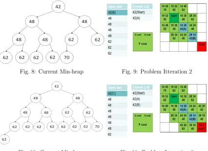
In the example given in Fig.7, A* is trying to find the path from the start location
to the goal location. After inserting the start node, A* will explore the neighbours of
this node, and it will select the node with the lowestf cost which is shown as “Node
A”. The current state of our Min-Heap is also is represented in Fig.6.
In the second iteration A*, extract the current minimum from the min-heap and
expand the neighbours of “Node B”(Fig.9). The current state of Min-Heap is shown
in Fig.8.
In this iteration, A* algorithm extracts the node with the minimumf value, Since
1. INTRODUCTION
Fig. 8: Current Min-heap Fig. 9: Problem Itteration 2
Fig. 10: Current Min-heap Fig. 11: Problem Itteration 3
will stop. Each time that a new insertion was made to the Min-Heap, based on
the data structure algorithm, the new node was inserted to the last place on the
data structure. After that, it was compared to its parent, and in case of having a
smaller value, the node swapped its location with its parent till that it finds its correct
location. The same function happened when we removed the minimum node from the
data structure. Based on the algorithm we swapped the last node’s location with the
node on top of the data structure, then checked if the node has a higher value than
its children, we swapped its location with them, till the nodes are in their correct
locations.
1. INTRODUCTION
expanded and they were not expanded during our search to find the shortest path. If
we limit the size of our data structure by limiting the depth of our Min-Heap, we could
have performed less number of operation such as Swap operations and comparisons
required by the Min-Heap to find the same path.
A* algorithm performance is limited due to the inserting a new node and
remov-ing the node with lowest f value operations. The algorithm inserts the expanded
neighbours of the current node if they are not in theclosed set and it will remove the
node with leastf value in theopen set. Hence the performance of the data structure
has a direct impact on the performance of the algorithm. Already existing solutions
for this problem is using a priority-queue which usually is a Min-Heap. A Min-Heap
requires O(log n) number of operations to maintain the properties of a min-heap.
In this research, we introduced two new solutions based on the min-heap, which
result in better performance in terms of operations and runtime in the right
circum-stances. The first solution is called Cached Min-Heap, which we took the idea from
the Heap On-Top Priority Queues, but based on our own implementation and is our
newly introduced algorithm. The second data structure that we implemented is the
Partial Min-Heap, which is an optimistic solution for this pathfinding problem which
under the right circumstances is able to find the correct optimal path with less number
of operation and better runtime in comparison to the Min-Heap.
1.8
Thesis Organization
This thesis paper is organized into 6 chapters. The first contains introductory
in-formation about the pathfinding algorithms and necessary inin-formation regarding the
A* algorithm and provides a small background about our work. The second chapter
mainly focuses on the previously introduced solutions to the A* data structure. In
the third chapter, we introduce our proposed data structures Cached min-heap and
Partial min-heap and provide detailed functions of these data structures and analysis
them. Our fifth chapter is a summary of our experiments combined with our test
1. INTRODUCTION
results to the other existing solutions to the open set. The sixth chapter provides a
summary of our analysis and concludes our work and the seventh chapter provide a
possible blueprint of what can be the continuation of this research and how it might
CHAPTER 2
Literature Review
2.1
A* Data Structure
The functionality of A* search algorithm is dependant on two data structures that
are utilized in the main loop of this search algorithm. A* repeatedly extracts the
node with the lowest f cost from it’s open set, examine its neighbours to find the
best subsequent node to explore till it finds the goal node. The main loop of this
algorithm maintains its operations using two data structure open set and closed set,
which their implementation is essential to the algorithm’s performance. A* algorithm
needs a data structure to maintain its open set to perform more efficiently. A*
algorithm does not need to revisit the already expanded nodes from its closed set if
the heuristic function is consistent.
A* search algorithm operations onopen setdata structure are as follows: “Insert”,
“Remove min”, “Contains”, and “Update Node”. In each iteration, the algorithm
removes the node with the lowest f value from the open set and explore all of the
adjacent neighbours to the current node. Then the algorithm move the current node
from theopen setto the closed set. The algorithm will check if the neighbours of the
current node are members of theopen set. This operation is the contains operation.
If they are not already a member of ouropen set, they will be inserted into the open
set. In case of the nodes being members of the open set, the algorithm will decide
based on their f value the next course of action. If the new f value is larger than
the existingf value, the node will be discarded. Otherwise, the existing node f value
2. LITERATURE REVIEW
node’s parent should be changed too.
In this chapter, we discuss the already existing solutions of theopen setandclosed
set implementations for the A* algorithm and their time complexity based n which
is the number of members in each data structure.
2.2
Closed Set
If the heuristic function used in the A* algorithm is consistent, the implementation
of the closed set will not have a direct impact on the performance of the algorithm.
The algorithm already expanded the nodes that are members of the closed set and
the purpose of keeping these nodes are preventing our algorithm to enter an infinite
loop state [David Rutter]. The closed set can be implemented as an array or a hash
table.
Operations required in theclosed setis mainly membership tests. Implementation
of the closed set using an array requires O(n) operations to return the membership
and using a hash table requiresO(1) operations. In this research, we used hash tables
to implement ourclosed setsince we were looking for an optimized solution and better
performance to our pathfinding problem.
2.3
Open Set
Since that the majority of operations in A* search algorithm occur on the nodes in
the open set, the algorithm is heavily dependant on the performance and efficiency
of this data structure and researchers mainly focused on many solutions for theopen
set. Since that mostly each solution focuses on a particular problem, it is hard to
compare them to each other. We mainly focused on inserting a new node, removing
2. LITERATURE REVIEW
2.3.1
Array
Using an array to implement the open set, one solution is that the elements in the
array are not sorted and the other solution is to be sorted.
Unsorted Array
Inserting a new node to an unsorted array takes O(1) operation. We add the node
at the last possible location in the array without any operations. Removing the node
with the lowest f value requires O(n) operations since we need to scan the array to
find the node with lowest f value. Contains is the same as removing a node from
the array and requires O(n) operations. Updating a node’s f value requires O(n)
operations as well since it needs to first find the node in the array, then change itsf
value.
Sorted Array
Since that the array requires to be sorted at any time during the operation, inserting
a new node requires O(n) operations. At first, the array needs to be scanned to find
the correct locations of the inserted node based on the f value; then the subsequent
nodes needs to be shifted to the new location. Removing the node with the lowestf
value requiresO(1) operation since that the array is sorted and the node at the index
or last location in the array is the minimum node. Finding the node in the array can
be implemented using different methods. Using binary search to find the node in the
array requiresO(log n) operations. Update method requiresO(n+log n) operations
since that we need to find the node then locate the correct position of the node in
the array.
2.3.2
Hash Table
Using hash tables to implement the open setwas suggested in this study [6] since it
allows the algorithm an instant accessing time. Inserting a new node, update and
2. LITERATURE REVIEW
requiresO(n) operation to find the node with the lowestf value. The data structure
should still follow the properties of a priority queue.
The main issue using a hash table is the indexing problem. In each search, items
in the hash table need to acquire a hash key which requires computational power
to calculate for each node. The developer needs to use the right hash algorithm to
prevent duplicated keys.
2.3.3
Binary Min-Heap
Min-heap is one of the most popular solutions to implement the open set which
was introduced in 1964 by Williams[1], is a complete binary tree which follows the
properties of a priority queue. Each item in the min-heap required to have an index
which allows the data structure to locate each node’s location in the tree. Using
an array (Fig.12) is one of the most popular ways to implement a binary min-heap.
Nodes in the min-heap must have smaller or equal value than their children nodes.
Min-Heap implements “Insert” and “Remove Min” functions.
2. LITERATURE REVIEW
Insert
To insert (Fig. 13) a new node to the heap, this data structure inserts the new node
to the last available location in the heap. Then it will check if the node is in the
correct location by checking if the node’s value is higher than its parent. If the node
has a smaller value, the location of the newly inserted node will be swapped with
its parent node. This operation usually is called the sort-up or bubble up operation.
Adding a new node requires O(log n) operations.
Fig. 13: Inserting to Min-Heap
Remove Min
To Remove the node with the min f value in the Min-Heap, this data structures
remove the node at the top of the tree, replace it with the node at the last index in
the tree. Then it will check if the node has a smaller value than any of its children.
The node with the least value will be swapped with the node on top till the node find
its correct location in the tree. This process also is called sort-down or bubble down
operation. Removing the minimum node requires O(log n) operations.
Contain and Update
To find the node which is the Contain operation in the min-heap, firstly we need to
traverse the array which requires O(n) operations. If the node needs to be updated,
first we find the node in the heap, then we update its value. Since that the node’s
2. LITERATURE REVIEW
Fig. 14: Remove Min - Min-Heap
of a Min-Heap and find the correct location of the node in the heap which requires
O(log n) operations.
2.3.4
Fibonacci Heap
Despite the promising time complexities of Fibonacci heap [11], this data structure
is not a popular solution to the A* shortest path problem due to the implementation
complexities of the Fibonacci heap. This data structure mainly developed to improve
the time complexity of Dijkstra’s algorithm but the authors mentioned that it could
be used as a priority queue in any problem. Fibonacci heap is a combination of
heap-ordered trees. Each sub tree is a non-binary min-tree which has a pointer of
its minimum member to a root list. Root list will keep track of all of the minimum
members of the sub trees and has a pointer to the minimum member in the entire
heap.
Insert and Remove
To add a new node to the Fibonacci heap, first, we create a singleton tree using that
node then we insert the new singleton tree into the root list. If the new singleton
2. LITERATURE REVIEW
Fig. 15: Fibonacci-Heap Insert Example
following operations. First, the algorithm extracts the minimum node, then meld its
children to the root list then consolidate the remaining trees so that no two roots
have the same rank.
2.3.5
Multilevel Buckets
Multilevel buckets [12] is using the bucket data structure which maintains an array
of buckets. In a data structure with K bucket levels, K = 0 is the lowest level, and K
= K-1 is the highest level of the bucket, in which each bucket only keeps the nodes
with certain value off. The algorithm will use theith bucket at the time and expand
the nodes correspond to that bucket. If the current bucket is empty, the algorithm
will use the next bucket with the values of f. In case of updating a node, the node
will be removed from its current bucket, and it will be moved to the new bucket
of its corresponding f value. Since that this data structure was introduced to work
with Dijkstra’s algorithm, there was no definition of the contain method. Based on
the implementation of this data structure, inserting and removing a node will take a
constant time based on the number of buckets used and the number of nodes.
2.3.6
MultiQueues
MultiQueues [21] is an array Q of multiple lock protected priority queues. In this data
2. LITERATURE REVIEW
Inserting a new node, will Lock the Q[i] priority queue and insert the element into
the priority queue. Since that the priority queue follows the properties of a binary
tree, Insert requires O(log n) + 1 operations where n is the number of node in the
Q[i]th priority queue. Operations required to delete the node with the lowest value is
similar to the insert functions with the difference that the node will be removed from
the priority queue with the smallest value. Operations required for the delete-min
operation in this data structure isO(log n) + 1 where nis the number of nodes in the
Q[i]th priority queue and plus one is the fixed operation of choosing the ith priority
queue.
2.3.7
Heap On Top Priority Queues
A combination of Multi-level bucket data structure of Denardo and Fox [8] with binary
min-heap data structure was introduced to improve the performance of Dijkstra’s
algorithm which is called heap on top priority queue [5]. Hot priority queue, is a data
structure combination of a heap H and the k-level bucket data structure B. Elements
of this data structure are either a member of H or B. Size of the heap section is
finite and is set to a n element which we assumed that is defined by the developer
based on the right circumstances since that the author did not mention a method
of calculating the n. Buckets are required to have a fixed size of K as well, and
they are unsorted arrays that are keeping the node with a specific value range. Since
that H is following the properties of a min-heap, Inserting a new node into the H
require O(log n) where isn is the number of nodes currently in the heap section and
if the value of the inserted node is outside of the specific range, insert requires O(1)
operation to complete the insertion process. Removing a node from the Hot queue
requires O(log n) operations where n is the number of nodes in the H. If the heap
section is empty, the algorithm uses the next unsorted bucket and convert its members
2. LITERATURE REVIEW
the heap section and it requiresO(log n) operation to locate it in the correct position.
If the node is inith bucket, the node will be removed and it will be inserted into the
correct bucket.
2.4
Summary
Each data structure that was mentioned in this chapter has its own advantages and
disadvantages. Based on the information gathered we could report the following
table (Table. 1) as a mean of comparison for these data structures in the primary
four operations needed for A* algorithm to operate.
Data Structures Insert Remove Min Contains Update
Unsorted Array O(1) O(n) O(n) O(n)
Sorted Array O(n) O(1) O(log n) O(n) +O(log n)
Hash Table O(1) O(n) O(1) O(1)
Min-Heap O(log n) O(log n) O(n) O(n) +O(log n)
Fibonacci Heap O(1) O(log n) O(1) O(1)
MultiQueue O(log n) + 1 O(log n) + 1 O(n) O(n) +O(log n)
Hot Queue O(log n/k) O(log n/k) or O(n) O(n) +O(log n/k)
or O(1) O(n/k) or O(n)
Table 1: Time Complexity Comparison of Different Data Structures
Performance of these data structures under the right circumstance is different.
Since that search algorithms belong to the NP-hard family problems, size of the
problem has a direct impact on the complexity of the solution. Performance of these
data structures might not be significantly different in small size problems. Another
important remark is the use of these data structures in the game industry. Although
that Fibonacci heap is better in terms of time complexity than the min-heap, due
to outstanding implementation challenges most of the games use min-heap instead.
2. LITERATURE REVIEW
them since that it requires hashing operations and prevent any key collisions. Heap
on top priority queue it could perform better under the right circumstances but since
that the author’s explanations were not clear we did not use it in our research. In
our study, we proposed our implementation of the Hot queue as cached min-heap and
also proposed our data structure partial min-heap and compared their result to the
CHAPTER 3
Cached Min-Heap and Partial
Min-heap
3.1
Motivation
Based on our studies in the field of pathfinding we explored multiple solutions
re-garding the A* search algorithm performance. Some of the solutions mainly focused
on the representation of the map, and they suggested that by decreasing the size
of the map and partially representing the map can increase the performance of this
algorithm. Some of the algorithms suggested different solutions based on single agent
or multiple agent pathfinding solutions. The operations that are related to the Open
setare the most resource consuming operations of this algorithm. Researchers
intro-duced a number of solutions for this problem, and each of these solutions relates to a
type of problem. Data structures such as the Hot queue, MultiQueue, and Multilevel
buckets suggested that by distributing the load of nodes into multiple sections and
data structures, our algorithm performs more efficiently which this idea motivated
us to exploit this research. Our experiments showed us that in a normal pathfinding
problem in a large fully connected graph, using an admissible and consistent heuristic,
the majority of the nodes inserted into the open set are not a part of the solution,
but the data structure performs a vast number of operations to keep them.
In our research, the agents were allowed to move in any direction with the set cost
of 10 for non-diagonal and 14 as the diagonal movement. The heuristic function used
3. CACHED MIN-HEAP AND PARTIAL MIN-HEAP
Fig. 16: Example of search environment
The green node is the start location and red is our goal location. Each cell has three
values written inside which the top-left value is the G cost, top-right is the H cost,
and the bottom value is the summary of given values asF cost as given in the Fig.16.
In the following examples, nodes in light green color are representing the nodes in the
open setand the nodes in blue are the nodes in the closed set. In our experiment we
used a min-heap to implement our open set.
In the first iteration, our A* search algorithm extract our start node from the
open set and explore its children and insert them into the open set. The algorithm
then extracts the node with the least f(Node A) cost and explore its children.
3. CACHED MIN-HEAP AND PARTIAL MIN-HEAP
observation. The f value of the nodes that directed us to the correct path was 42,
and they did not change in the pathfinding process.
Fig. 18: Example of search environment (Exploring a node)
Data structure before finding the goal node has 16 members. Most of the members
in the current heap were not explored, but the data structure kept them as members.
Since that these nodes are members of this heap, the current depth of this min heap
is 5. In case that we want to remove the minimum node from this data structure,
min-heap will return the current minimum node, and it will replace it with the last
node in the heap, and perform the required operations to find the correct location of
it.
Since that the current heap has 16 members and the time complexity of the
min-heap is O(log n), removing the minimum node requires four operations. In a
pathfinding problem, children of the current node have the same f value or f + d
values where dis the distance of the current node to the next node if our heuristic is
consistent. Based on the aforesaid, binary heap expects values smaller or relevantly
small values in comparison to the nodes at the bottom part of the heap. In the
following example, you can see that the nodes at the bottom of the heap have values
of “62” whereas the nodes inserted have values of “48” and “42”. The worst case
operation for inserting a new node into the heap is O(log n), and in this example, it
requires “4” operations to locate the newly inserted node into the heap.
Based on the given example we can observe that:
3. CACHED MIN-HEAP AND PARTIAL MIN-HEAP
in the worst case complexity of the min-heap which is O(log n).
- The majority of the inserted nodes are irrelevant to the pathfinding solution.
These nodes only increase the size of the heap, hence expanding the time complexity
of the algorithm.
It is clear that if we decrease the size of our data structure, we decrease the time
complexity of our min-heap and increase its performance. Based on our second
obser-vation we came up with a theory that our pathfinding algorithm might be successful
to find the correct optimal path if we limit the memory size of our data structure.
Based on our observations and the concept of multiqueues combined with multi-level
bucket data structure, we came up with two new data structures to implement the
open set for the A* search algorithm, Cached min-heap and Partial min-heap.
Our cached min-heap divide the data structure into logically two sections in one
array, where each element of the array has an index which we took the original idea
from the heap on top priority queue. The cached min-heap first section follows the
properties of a min-heap and the second section is an unsorted array. The first section
of this data structure serves the A* algorithm till there are no new nodes inside, If this
section is empty, then our algorithm will use quick sort to build the heap section using
the members in the reserved section. Our partial min-heap is an optimistic min-heap
data structure which helps the A* algorithm to find the solution performing fewer
operations since it limits the search space by eliminating nodes that have a higherf
value. Both data structure are explained in detail in the following sections.
3.2
Cached Min-Heap
Based on the idea of Hot queues and Multilevel buckets, we proposed a data structure
called Cached min-heap. This data structure logically separates itself to two sections
3. CACHED MIN-HEAP AND PARTIAL MIN-HEAP
of elements in the heap is 2d−1 elements.
We designed cached min-heap in a way that the elements inside the heap always
have values smaller than the reserved section. To achieve this goal since that we want
our algorithm to function correctly, we keep a pointer to the minimum element in our
cached section. Also, we keep a pointer to the maximum node in our heap section as
well.
Fig. 19: Cached Min-Heap Data Structure d=3
3.2.1
Cached Min-Heap Operations
Cached min-heap is designed to improve the performance of A* algorithm data
struc-ture and satisfies the main four operations required. In the following we explained
and analysed the required operation which are Insert, Remove-Min, Contains, and
Update based on n where n is the number of nodes in the data structure.
Insert
For Inserting an element, cached min-heap follow certain steps to insert the new node
into the data structure. If the heap has empty space and the reserved section is also
empty, the new nodes will be inserted into the heap section. If the inserted node has
3. CACHED MIN-HEAP AND PARTIAL MIN-HEAP
in Figure 20, inserting the new node with the value of 62 the node will be inserted
to the last space available in the heap section. The new node has a higher value in
comparison to its parent, so it is in the correct location. Since that the new node has
higherf value than the node with the index of “4” (old max node), the maxpointer
will be set to the new node in the heap.
Fig. 20: Cached Min-Heap Data Structure Example d=3
If the heap has empty space but our reserved section has elements inside, the data
structure checks if the new nodes f value is smaller than the current min item in
the reserved section. If it has smaller value, the node will be inserted into the heap
section. Otherwise, it will be inserted into the reserved section. For example in the
Figure 21, the reserved section has “70 & 80” as members and 70 is themin member
of our reserved section and our heap section has empty space. The algorithm will
check the new member f value and compare it to the min member in the reserved
section. Since that it has a higher value than our current min the node will be
inserted to the reserved section.
If the heap is full and we are inserting a new node, the data structure will compare
3. CACHED MIN-HEAP AND PARTIAL MIN-HEAP
Fig. 21: Cached Min-Heap Data Structure Example d=3
and change the pointer to that node. For example in Figure.22, the new node has
f value of “48” which is smaller than the current max node with the value of “62”.
The algorithm will replace the new node with the old max node and insert the old
maxinto the reserved section.
Fig. 22: Cached Min-Heap Data Structure Example d=3
In this example (Fig. 22), the algorithm will check if the newly inserted node
into the reserved section is smaller than the current min or not if it is smaller it will
replace the current minwith the newly inserted node. Since that we replaced the old
3. CACHED MIN-HEAP AND PARTIAL MIN-HEAP
the node in the index “6” in the heap section and change themaxpointer to the new
maxnode.
Since that cached min-heap data structure follows the mentioned steps to insert
a new node, it is guaranteed that at any stage, the element of the heap section has
smallerf value than the reserved section. The time complexity of our insert operation
is O(log n) if the heap has empty space, O(1) if the heap is full and the node has
higher f value than the maxvalue in the heap. If the heap is full and the new node
has smaller f value, inserting the node needs O(log n) + 1 operations to replace the
node in the heap and place it in the reserved section and it needs O(n/2) operations
to find the max node in the leaf nodes of the heap section.
Remove Min
Cached min-heap requiresO(log n) operations to remove a node from the heap section
since it follows the properties of a min-heap in the top section. In case that the top
section of our data structure is empty, our algorithm will perform the Quicksort
algorithm on the reserved section and replenish our heap section using the nodes
from our reserved section. We understand that this operation is computationally
heavy and requires O(n log(n)) average operation to sort the data and insert them
to the heap and then it needs O(log n) operations to remove the minimum node.
A* algorithm usually inserts more nodes and extract less number of nodes during
a pathfinding problem, and if our algorithm requires to perform this operation, the
performance will suffer heavily. We expect that this operation does not happen many
times during a pathfinding solution.
Contains
Elements in the data structure are representing objects of a node. During the
3. CACHED MIN-HEAP AND PARTIAL MIN-HEAP
for the new node. For example in Figure.23 the algorithm needs to scan each element
at the indexes to find out the new node is a duplicate node or not.
Fig. 23: Cached Min-Heap Data Structure Contains
Update
In our cached min-heap data structure we logically separate the data, so the nodes
are either in the heap section of data structure or they are in the reserved section of
our data structure. First, we need to locate the node in our data structure which is
the same operation as the contains operation which requires O(n) operations. If the
located node is in our heap section, we treat it as a min-heap operation which requires
O(log n) operation to find the correct location for the new node in the heap. If the
node is located in our reserved section, we first change the f value then compare it
with themaxnode in our heap section. If the newf value is smaller than the current
max, we replace themaxnode with the current node and check to find the newmax
value in our heap section. Since that we inserted a new node into the reserved section
we check if the new node is smaller than the current min or not, if it is we update
the new min pointer to the new min node.
Replenish Cache
During a pathfinding problem, if our heuristic function is consistent and our search
environment is clear of obstacles along the way, the expanded nodes of the current
node are guaranteed to have smaller f values. If our search environment contains
multiple path blocks along the optimal path suggested by our heuristic, the nodes
3. CACHED MIN-HEAP AND PARTIAL MIN-HEAP
will result in inserting nodes with a higher value than the current min node and
performing more remove-min operations from the heap section and inserting a node
in the reserved section. Since that this series of operations are a regular part of
a pathfinding problem, we implemented our method to refill the cache section of
our data structure. Our first solution to this problem was to perform a build-heap
operation which only takes O(log n) operations. After implementing the replenish
cache method using heap sort we noticed that of our A* algorithm is not functioning
correctly. We noticed that using the heap sort to replenish our cached part and slicing
our data structure to two sections is not guaranteed to work correctly since we might
have a node with smaller values in the reserved section that they belong to the heap
part. You can see in the given example below (Fig. 24) that slicing the data structure
to a depth of 3; we will have nodes that are smaller in the reserved section, so we
3. CACHED MIN-HEAP AND PARTIAL MIN-HEAP
Summary
Based on our analysis of the operations of cached min-heap, we can state that the
performance of this data structure depends on two main components. First is the
depth of the data structure and second is the replenish cache operation. If the depth
of this data structure is small, the data structure will save some operations since
that the size of the heap is smaller than a min-heap but the numbers of calling the
replenish cache will be increased.
3.3
Partial Min-Heap
Based on our experiments we observed that a majority of nodes in the data structure
are not related to the path that A* algorithm finds. Our second observation was
that the depth of the min-heap has a direct impact on the performance of the data
structure. We proposed a new data structure called partial min-heap which is an
optimistic data structure for the A* algorithm. We estimated that this data structure
performs better than min-heap under the right circumstances with a high chance of
successfully returning an optimal path. Same as cached min-heap we assigned an
index to each element in the data structure, and we also set a maximum size for this
data structure as well. The maximum number of elements in this data structure is
2d−1 whered is the depth of the data structure.
3.3.1
Partial Min-Heap Operations
Partial min-heap is an optimistic data structure which aims to limit the search space
of the A* algorithm while following the properties of a min-heap. This data structure
performs the main operations required by the A* algorithm. In the following section,
3. CACHED MIN-HEAP AND PARTIAL MIN-HEAP
Insert
Since that this data structure only contains a limited number of nodes at the time,
First the algorithm checks if the data structure is full or has empty space. If the data
structure is empty, the first inserted node will be inserted into the heap, and its value
will be set to the max value and the index of that node will be saved. If the data
structure is not full, the nodes that the A* algorithm insert them into the heap will
be added to the partial min-heap same as the min-heap. In each insertion operation,
we check if the current node f value is higher than the current max node. If it is
higher, after that we locate the correct position of the node, we will set the pointer
of the new max node to the newly inserted node. If our data structure is full, we
compare the f value of the inserted node to the current max nodes f value. If the
new node has a higherf value, we discard the new node and if it has a smallerf value
compare to the current max node, we replace the new node with the current max
node’s location which isO(1) operation to replace the node and O(log n) operations
to relocate the inserted node to its correct location. Since that we replace the max
node, we need to find the newmaxnode in the heap so we scan the leaf nodes to find
the new max location which requires O(n/2) operations.
For example in the Figure. 25, the new node has af value of “48” which is smaller
than the current max node with the value of “60”. The algorithm will replace the
new node with the old maxnode and discard the oldmaxnode. Then the algorithm
will scan the leaf node in the current heap and find the new max item which is the
node in the index “3”.
Remove Min
Partial min-heap requiresO(log n) operations to remove a node from the heap section
3. CACHED MIN-HEAP AND PARTIAL MIN-HEAP
Fig. 25: Partial Min-Heap Data Structure Insert Example d=3
Fig. 26: Partial Min-Heap Data Structure Remove Min Example d=3
For example in the Figure. 26, first partial min-heap extract the minimum node
with the value of “42”, then replace that node with the last node in the index of “6”
in the heap. Then compare its value with its children, since that the node has a value
equal to its children no operation is required, and the node is in the correct location.
Contains
The same as the cached min-heap data structure, elements that are members of the
partial min-heap are objects of type node. To locate a node in the data structure, we
need to compare the node in the matter with each node in the heap to ensure if the
node is already a member of the data structure or not. This operation takes O(n) to
3. CACHED MIN-HEAP AND PARTIAL MIN-HEAP
Update
Scanning the entire data structure requires O(n) operation to find the node that we
need to update, then we change thef value of the updated node. Since that the new
value might not be in the correct position in the heap and violate the properties of
the min-heap, we need O(log n) operations to locate the updated node in its right
location in the heap.
3.4
Partial Min-Heap Case study
Partial min-heap is designed to decrease the size of the memory in our A* pathfinding
algorithm. Since that we are techinically limiting the search space for our algorithm
we will face the risk of losing the optimallity of the path or failure of finding the path.
3.4.1
Partial Min-Heap Success
In the following example, we set the depth of the partial min-heap tod= 3. Based on
the formula that we provided, Partial min-heap at most will accept 23−1 = 7 elements
at most. Since that we limited the number of nodes so in each insert operation and
remove min operation we will save extra operations compare to d = 5 depth. In
the example given bellow we can see the final iteration of A* algorithm finding the
path using a min-heap as open set. In this example, our min-heap accepts all of the
inserted nodes. Our assumption was that using the correct d and limiting the size of
the data structure will result in an optimal or sub-optimal path. If we set the limit
of size of the data structure to d= 3 in figure 27, our pathfinding algorithm intially
inserts neighbours of the starting node, since that the data structure will be filled
out with the neighbours of the start node, The node with thef value of “70” will be
3. CACHED MIN-HEAP AND PARTIAL MIN-HEAP
Fig. 27: Pathfinding Example
replace them with the new nodes with smaller f values.
Fig. 28: Pathfinding Example
In the last iteration shown in Figure. 29 you can see that A* algorithm was able
to find the optimal path using the partial min-heap data structure while discarding
nine extra nodes. Our pathfinding performed less number of compare operations since
that worst case for each insert and remove operation was O(log 8) compare to the
O(log 15) operations in a normal min-heap in the last iteration of this pathfinding
example. So our expectation is that the partial min-heap will let us to be able to find
3. CACHED MIN-HEAP AND PARTIAL MIN-HEAP
Fig. 29: Pathfinding Example
3.4.2
Partial Min-Heap Failure or Sub-optimallity
Same rule applies if we slice our data structure too small and set a small size data
structure for a problem. If our data structure is too small, our A* algorithm might
try to re-insert the already discarded nodes into the data structure which might result
in finding a path to the goal node. In case of this issue ocurring, our solution to this
problem will be suboptimal since we might have missed the branch in our graph that
was resulting in the shortest path. If our data structure is smaller than a certain size
or our map has large blocks along in the path, our data structure will compeletly fail
to find an answer since it already discarded the nodes that will result in finding a
path out of the blockage.
3.4.3
Summary
Our proposed partial min-heap is an optimistic data structure for the open set for
the A* pathfinding algorithm. Our analysis of this data structure is that if the depth
of the data structure which represents the size of it, has a crucial role in the success
or failure of the pathfinding algorithm. Limiting the size of the data structure to