ABSTRACT
ARNOLD, LAURA ANN. Effects of Drain Depth on Nitrogen Losses in Drainage in Shallow Water Table Soils. (under the direction of R. Wayne Skaggs).
A two-part study (a field study and a modeling study) was undertaken to investigate the effect of shallow subsurface drains on nitrate-nitrogen (NO3-N) losses in drainage effluent
relative to deep subsurface drains. The field study was conducted in the Lower Coastal Plain of North Carolina over a two year period between May 12, 2001 and April 30, 2003. Crops grown on the site were corn in 2001 followed by wheat and soybean in 2001/2002. The field was nearly flat and the soils were Portsmouth sandy loam and Cape Fear loam, which, under natural conditions are very poorly drained. The site was subdivided into eight 1.8 ha plots, each drained by three parallel drains spaced 23 m apart. Drains in plots one through three were shallow with an average drain depth of 0.86 m. Drains in plots four through six were deeper, with an average depth of 1.20 m.
Precipitation, water table depth and subsurface drainage rates were measured
continuously during the study. Subsurface drainage was sampled and analyzed to determine NO3-N concentration in the effluent. Measurements of water table depth and subsurface
drainage quantity and quality were made within each plot.
Drain depth had no statistically significant effect on drainage water quality. For Year 1, the average NO3-N losses from the shallow drains and deep drains were 21.7 and 28.0 kg ha-1,
respectively. For Year 2, the average NO3-N losses from the shallow and deep drains were 28.9
and 23.5 kg ha-1 respectively. For the entire study period, total average NO3-N loss from the
shallow drains was 50.6 kg ha-1 and the total average loss from the deep drains was 51.5 kg ha-1. Observed behavior in shallow plot 2 was an anomaly. More subsurface drainage
occurred and more NO3-N was lost from plot 2 than any other plot. Based on analysis performed
in conjunction with predicted results from the modeling study, it was determined that plot 2 was not hydraulically isolated and was receiving surface runoff from an adjacent plot.
EFFECTS OF DRAIN DEPTH ON NITROGEN LOSSES IN DRAINAGE
IN SHALLOW WATER TABLE SOILS
by
LAURA A. ARNOLD
A thesis submitted to the Graduate Faculty North Carolina State University
in partial fulfillment of the requirements of the Degree of
Master of Science
BIOLOGICAL AND AGRICULTURAL ENGINEERING
Raleigh
2004
APPROVED BY:
--- ---
Dr. R. Wayne Skaggs Dr. Michael Vepraskas
Chair of Advisory Committee Minor Representative
---
Dr. George M. Chescheir
D
EDICATIONThis thesis is dedicated to:
Nessa Stone, my life partner, who has so patiently supported me during this long
process. She has given so much to make this possible.
B
IOGRAPHYLaura Ann Arnold was born September 26, 1969 in Lexington, Kentucky. She is the
youngest of three children of Nicholas and Carolyn Arnold. She attended Lafayette High
School in Lexington, where she lettered in softball three years and played flute in the band.
After graduation, she attended The American University in Washington, DC for one year. In
search of life experience, she left school, worked a variety of jobs, and played bass guitar in a
band.
In 1995, she entered the University of Kentucky to complete her education and gain a
degree that would allow her to work in the environmental field. On the recommendation of
her brother, a UK Agricultural Engineering alumnus, she chose the Biosystems and
Agricultural Engineering Department. She graduated cum laude with a Bachelor of Science
degree in Biosystems and Agricultural Engineering in May, 2000. The emphasis of the
degree program was bioenvironmental studies.
In August 2000, she moved to Raleigh, North Carolina to pursue a Master’s degree
A
CKNOWLEDGEMENTSI would like to acknowledge the following people who have contributed to the completion of
this study:
Dr. Wayne Skaggs for providing the opportunity and sharing his tremendous understanding
of all things relating to drainage. He also provided generous financial support during the
long course of this project.
Dr. Chip Chescheir for always taking the time to answer my questions and offer suggestions
when I was at a loss.
Dr. Mike Vepraskas for serving as minor representative on my graduate committee.
Dr. Mohamed Youssef for his great support and encouragement when the project was at a
standstill and for his patience as a teacher.
Jay Frick for his hard work in retrieving all field data, maintaining the field equipment and
for his friendship and great sense of humor. It lifted my spirits many days.
Wilson Huntley for collecting the water quality samples and assistance in maintaining the
experimental equipment.
I also would like to offer my great appreciation to the people who supported me personally:
My aunt, Barbara Tiabian, who offered much support and encouragement. She always
listened and believed.
To my grandparents and great-grandparents, who began building the foundation of our
family when they came to the United States to seek better opportunity for themselves and
T
ABLE OFC
ONTENTSList of Tables... viii
List of Figures... xi
Chapter 1: Effect of Drain Depth on Nitrogen Losses in Drainage Water...1
INTRODUCTION...1
Hydrologic and water quality changes with artificial drainage ...3
Controlled Drainage...4
Denitrification ...5
Shallow Drains...6
MATERIALS AND METHODS...10
Site Description...10
Data Collection ...12
Precipitation ...12
Water Table Depth...13
Subsurface Drainage ...14
Water Quality Analysis...17
Cropping and Fertilization ...17
RESULTS AND DISCUSSION...18
Hydrology ...18
Nitrogen ...27
SUMMARY AND CONCLUSION...29
REFERENCES...65
Chapter 2: Simulation Study to Evaluate Effect of Shallow Subsurface Drains on Nitrate Losses in Drainage Effluent...68
INTRODUCTION...68
MATERIALS AND METHODS...69
Site Description...69
Hydrologic Model Description ...69
Nitrogen Model Description ...70
PROCEDURE...71
Short Term Simulation Study - Hydrologic Model Parameterization ...72
Organic Nitrogen Input Parameters for DRAINMOD-N II...79
Plant Uptake Parameters for DRAINMOD-N II ...80
Rooting Depth Parameters for DRAINMOD-N II...80
Nitrogen Transport Parameters for DRAINMOD-N II ...81
Nitrogen Transformation Parameters for DRAINMOD-N II ...81
Organic Matter Parameters for DRAINMOD-N II...81
Initialization Parameters for DRAINMOD-N II...81
Long Term Simulation Study - Hydrologic Model Parameterization ...82
Long Term Simulation Study - Nitrogen Model Parameterization ...83
Crop Input Parameters for DRAINMOD-N II...83
Fertilization (Mineral Nitrogen) Input Parameters for DRAINMOD-N II ...83
Organic Nitrogen Input Parameters for DRAINMOD-N II ...84
RESULTS AND DISCUSSION...84
Short Term Simulation Study – Hydrology ...84
Short Term Simulation Study - Nitrogen...88
Long Term Simulation Study – Hydrology ...89
Long Term Simulation Study – Nitrogen ...90
CONCLUSION...93
REFERENCES...149
Appendix A: Field Measurements...151
Appendix B: Measured Meteorological Data...183
L
IST OFT
ABLESChapter 1
Table 1.1. Average annual results from 50-year DRAINMOD simulation comparing deep and shallow subsurface drains using
meteorological data collected at Tidewater Research.
Station, Plymouth, NC. ...32
Table 1.2. Drainage system characteristics of experimental plots from research site at Tidewater Research Station, Plymouth, North Carolina. ...32
Table 1.3. Cropping and fertilization schedule during drain depth experiment...32
Table 1.4. Monthly measured precipitation during drain depth experiment at Tidewater Research Station, Plymouth, NC. ...33
Table 1.5. Average Quarterly Water Table Depths. ...33
Table 1.6. Measured monthly subsurface drainage depths from drain depth experiment...34
Table 1.7. Measured nitrate nitrogen concentration in drainage effluent (mg/L)...35
Table 1.8 Nitrate-nitrogen losses via subsurface drainage. ...36
Table 1.9 Flow weight average concentration of nitrate-nitrogen measured in subsurface drainage. ...36
Chapter 2 Table 2.1. Monthly estimated PET at the Tidewater Research Station. ...95
Table 2.2. Drainage system parameters for plots 2 – 6...95
Table 2.3. Lateral Saturated Hydraulic Conductivity for plots 2 - 6. ...95
Table 2.4. Water table depth – upward flux relationship for plots 2 - 6...96
Table 2.5. Water table depth – volume drained relationship for plots 2 – 6...97
Table 2.6. Green & Ampt infiltration equation coefficients for plots 2 – 6...98
Table 2.7. Crop effective rooting depths for plots 2 -6...99
Table 2.20. Fertilization input parameters (kg ha-1). ...105
Table 2.21. Calculated straw yield (kg ha-1)...106
Table 2.22. Calculated below ground biomass (kg ha-1). ...106
Table 2.23. Chemical composition of crop residues...106
Table 2.24. Nitrogen uptake function ...107
Table 2.25. Nitrogen transport parameters...107
Table 2.26. Transformation parameters - Nitrification. ...107
Table 2.27. Transformation parameters - Denitrification. ...108
Table 2.28. Transformation parameters – Fertilizer dissolution...108
Table 2.29. Transformation parameters – Urea hydrolysis...108
Table 2.30. Organic matter parameters...109
Table 2.31. Organic carbon decomposition parameters...109
Table 2.32. Organic Matter pools and total organic carbon, initial parameters...109
Table 2.33. Initial total organic carbon distribution in profile...110
Table 2.34. Initial conditions. ...110
Table 2.35. Long term simulation cropping sequence and fertilization table...111
Table 2.36. Statistical comparison of observed and predicted water table depth...112
Table 2.37. Statistical comparison of observed and predicted subsurface drainage rates. ...113
Table 2.38. Observed and predicted annual subsurface drainage. ...113
Table 2.39. Observed and predicted annual nitrate-nitrogen losses. ...114
Table 2.40. Predicted subsurface drainage totals – long term simulation...114
Table 2.41. Predicted surface drainage totals – long term simulation. ...114
Table 2.42. Predicted evapotranspiration totals – long term simulation...113
Table 2.43. Predicted infiltration totals – long term simulation. ...115
Table 2.44. Predicted relative yields for deep and shallow drains...115
Table 2.45. Predicted annual rates (kg N ha-1) of fertilization application, net mineralization, plant uptake, denitrification, and NO3-N drainage loss for Plot 2 ...116
Table 2.46. Predicted annual rates (kg N ha-1) of fertilization application, net mineralization, plant uptake, denitrification, and NO3-N drainage loss for Plot 3. ...117
Table 2.47. Predicted annual rates (kg N ha-1) of fertilization application, net mineralization, plant uptake, denitrification, and NO3-N drainage loss for Plot 4. ...118
Table 2.48. Predicted annual rates (kg N ha-11) of fertilization application, net mineralization, plant uptake, denitrification, and NO3-N drainage loss for Plot 5. ...119
Appendix A
Table A.1. Measured daily subsurface drainage for Year 1 (May 12, 2001
to April 30, 2002)...151
Table A.2. Measured daily subsurface drainage for Year 2 (May 1, 2002 to April 30, 2003)...159
Table A.3 Measured daily water table depth at end of day for Year 1. ...167
Table A.4. Measured daily water table depth at end of day for Year 2. ...175
Appendix B Table B.1. Measured Hourly Rainfall used as DRAINMOD input...183
Table B.2. Daily maximum and minimum temperature for 2000. ...186
Table B.3. Daily maximum and minimum temperature for 2001. ...187
Table B.4. Daily maximum and minimum temperature for 2002. ...188
Table B.5. Daily maximum and minimum temperature for 2003. ...189
Table B.6. Daily potential evapotranspiration for 2000 and 2001 calculated with Penman Monteith method. ...190
Table B.7. Daily potential evapotranspiration for 2002 and 2003 calculated with Penman Monteith method...191
Appendix C Table C.1. Winter wheat growth stages and crop susceptibility factors for excess water stress...194
Table C.2. Winter wheat growing season during simulation period. ...194
Table C.3. Winter wheat physiological growth stages and yield response factor ...194
L
IST OFT
ABLESChapter 1
Figure 1.1. Annual average water table depths for a 50-year period as
predicted by DRAINMOD for two drain depths. ...38
Figure 1.2. Annual subsurface drainage for a 50-year period as predicted by DRAINMOD for two drain depths. ...38
Figure 1.3. Annual surface runoff for a 50-year period as predicted by DRAINMOD for two drain depths. ...39
Figure 1.4. Annual evapotranspiration for a 50-year period as predicted by DRAINMOD for two drain depths. ...32
Figure 1.5. Experimental site at Tidewater Research Station, near Plymouth, North Carolina. ...40
Figure 1.6. Soils Map of experimental site at Tidewater Research Station, Plymouth, North Carolina...41
Figure 1.7. Subsurface drain line design (single plot)...41
Figure 1.8. Weather station by Plot 5 instrument house. ...42
Figure 1.9. Water table recorder...42
Figure 1.10. Water table recorder with chart...43
Figure 1.11. Guard tank and center line tank arrangement in instrument house...43
Figure 1.12. Center line tank with flow volume measurement systems...44
Figure 1.13. Cumulative rainfall for Year 1 as measured by three gages and long term cumulative monthly average at Tidewater Research Station...45
Figure 1.14. Cumulative rainfall for Year 2 as measured by three gages and long term cumulative monthly average at Tidewater Research Station...45
Figure 1.15. Monthly and cumulative rainfall totals for Year 1, Year 2 and long term average for Plymouth, NC. ...46
Figure 1.16. Observed water table depth, May 2001 – July 2001...46
Figure 1.17. Observed water table depth, August 2001 – October 2001. ...47
Figure 1.18. Observed water table depth, November 2001 – January 2002. ...47
Figure 1.19. Observed water table depth, February 2002 – April 2002...48
Figure 1.20. Observed water table depth, May 2002 – July 2002...48
Figure 1.21. Observed water table depth, August 2002 – October 2002. ...49
Figure 1.22. Observed water table depth, November 2002 – January 2003. ...49
Figure 1.23. Observed water table depth, February 2003 – April 2003...50
Figure 1.24. Cumulative drainage depths for Year 1 ...51
Figure 1.25. Cumulative drainage depths for Year 2 ...51
Figure 1.26. Monthly subsurface drainage depths, Year 1...52
Figure 1.27. Monthly subsurface drainage depths, Year 2...52
Figure 1.32. Observed subsurface drainage rate versus height of water table
between drains for Plot 2 ...55
Figure 1.33. Observed subsurface drainage rate versus height of water table between drains for Plot 3. ...56
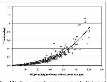
Figure 1.34. Observed subsurface drainage rate versus height of water table between drains for Plot 4. ...56
Figure 1.35. Observed subsurface drainage rate versus height of water table between drains for Plot 5. ...57
Figure 1.36. Observed subsurface drainage rate versus height of water table between drains for Plot 6. ...57
Figure 1.37. Drainage rate – height of water table relationship for shallow drains. ...58
Figure 1.38. Drainage rate – height of water table relationship for deep drains. ...58
Figure 1.39. Drainage rate – water table depth relationship for Plot 1 for two drain depths. ...59
Figure 1.40. Drainage rate – water table depth relationship for Plot 2 for two drain depths. ...59
Figure 1.41. Drainage rate – water table depth relationship for Plot 3 for two drain depths. ...60
Figure 1.42. Water table response – Storm Event 1...61
Figure 1.43. Measured drainage rate – Storm Event 1 ...61
Figure 1.44. Water table response –Storm Event 2...62
Figure 1.45. Measured drainage rate –Storm Event 2...62
Figure 1.46 Cumulative nitrate nitrogen (NO3-N) losses from subsurface drains, Year 1 (May 12, 2001 – April, 30 2002)...63
Figure 1.47. Cumulative nitrate nitrogen (NO3-N) losses from subsurface drains, Year 2 (May 1, 2002 – April, 30 2003)...63
Figure 1.48 Average cumulative nitrate nitrogen (NO3-N) losses from subsurface drains, Year 1 (May 12, 2001 – April, 30 2002). ...64
Figure 1.49 Average cumulative nitrate nitrogen (NO3-N) losses from subsurface drains, Year 2 (May 1, 2002 – April, 30 2003). ...64
Figure 2.10. Water table depth scatter diagram for Plot 3, Year 1...126
Figure 2.11. Cumulative rainfall, evapotranspiration, subsurface drainage and surface runoff for Plot 3, Year 1. ...127
Figure 2.12. Subsurface drainage scatter diagram for Plot 3, Year 1...127
Figure 2.13. Observed and predicted water table depths for Plot 3, Year 2...128
Figure 2.14. Water table depth scatter diagram for Plot 3, Year 2...128
Figure 2.15. Cumulative rainfall, evapotranspiration, subsurface drainage and surface runoff for Plot 3, Year 2. ...129
Figure 2.16. Subsurface drainage scatter diagram for Plot 3, Year 2...129
Figure 2.17. Observed and predicted water table depths for Plot 4, Year 1...130
Figure 2.18. Water table depth scatter diagram for Plot 4, Year 1...130
Figure 2.19. Cumulative rainfall, evapotranspiration, subsurface drainage and surface runoff for Plot 4, Year 1. ...131
Figure 2.20. Subsurface drainage scatter diagram for Plot 4, Year 1...131
Figure 2.21. Observed and predicted water table depths for Plot 4, Year 2...132
Figure 2.22. Water table depth scatter diagram for Plot 4, Year 2...132
Figure 2.23. Cumulative rainfall, evapotranspiration, subsurface drainage and surface runoff for Plot 4, Year 2. ...133
Figure 2.24. Subsurface drainage scatter diagram for Plot 4, Year 2...133
Figure 2.25. Observed and predicted water table depths for Plot 5, Year 1...134
Figure 2.26. Water table depth scatter diagram for Plot 5, Year 1...134
Figure 2.27. Cumulative rainfall, evapotranspiration, subsurface drainage and surface runoff for Plot 5, Year 1. ...135
Figure 2.28. Subsurface drainage scatter diagram for Plot 5, Year 1...135
Figure 2.29. Observed and predicted water table depths for Plot 5, Year 2...136
Figure 2.30. Water table depth scatter diagram for Plot 5, Year 2...136
Figure 2.31. Cumulative rainfall, evapotranspiration, subsurface drainage and surface runoff for Plot 5, Year 2. ...137
Figure 2.32. Subsurface drainage scatter diagram for Plot 5, Year 2...137
Figure 2.33. Observed and predicted water table depths for Plot 6, Year 1...138
Figure 2.34. Water table depth scatter diagram for Plot 6, Year 1...138
Figure 2.35. Observed and predicted water table depths for Plot 6, Year 1...139
Figure 2.36. Subsurface drainage scatter diagram for Plot 6, Year 1...139
Figure 2.37. Observed and predicted water table depths for Plot 6, Year 2...140
Figure 2.38. Water table depth scatter diagram for Plot 6, Year 2...140
Figure 2.39. Cumulative rainfall, evapotranspiration, subsurface drainage and surface runoff for Plot 6, Year 2. ...141
Figure 2.40. Subsurface drainage scatter diagram for Plot 6, Year 2...141
Figure 2.41. Observed and predicted subsurface drainage and nitrate-nitrogen loss from Plot 2. ...142
Figure 2.45. Observed and predicted subsurface drainage and
nitrate-nitrogen loss from Plot 6. ...144 Figure 2.46. Predicted subsurface drainage and surface runoff for
shallow and deep drain depths, Plot 4...145 Figure 2.47. Predicted evapotranspiration for shallow and deep drain
depths, Plot 4...145 Figure 2.48. Predicted nitrate nitrogen losses in subsurface drainage
for shallow and deep drain depths, Plot 4. ...146 Figure 2.49. Predicted denitrification for shallow and deep drain
depths, Plot 4...146 Figure 2.50. Nitrate-nitrogen additions, losses and storage for Plot 3,
November 1, 1991 to April 30, 2003. ...147 Figure 2.51. Nitrate-nitrogen additions, losses and storage for Plot 4,
November 1, 1991 to April 30, 2003 ...147 Figure 2.52. Nitrate-nitrogen additions, losses and storage for Plot 5
November 1, 1991 to April 30, 2003 ...148 Figure 2.53. Nitrate-nitrogen additions, losses and storage for Plot 6
I. Effect of Drain Depth on Nitrogen Losses in Drainage Water
INTRODUCTION
Water quality is an environmental issue of major concern in North Carolina,
nationally, and internationally. Both groundwater and surface water have become
contaminated in numerous locations as result of industrial, municipal and agricultural
activities. Significant effort and money have been spent to determine the sources of
contamination and methods to mitigate the resulting problems. One of the major
contaminants of ground and surface water is nitrogen. Drinking water contamination,
eutrophication of streams and rivers and hypoxia problems are associated with excessive
level of nitrogen in surface waters (Gilliam et al., 1999). A great deal of focus in the past has
been on addressing point source pollution, such as municipal wastewater treatment plants, as
they are more easily identified and monitored. For some time, non-point sources, such as
agriculture, have also received attention.
In agriculture, the primary source of nitrogen is fertilizer. Nitrogen that is not taken
up by the crop may leach into aquifers or be transported from the field by seepage or
subsurface drainage directly to surface water. Agriculture is responsible for over half of the
nutrients reaching surface waters in North Carolina (Department of Environment, Health and
Natural Resources of North Carolina, 1992). Eutrophication in the Neuse River and coastal
Mississippi River has received much attention. The area drained by the Mississippi is 3
million km2. The outlet for the river is the Gulf of Mexico. Mitsch et al. (2001) report that a
direct connection exists between the large quantities of nitrogen in the river and the hypoxic
area now found in the northern Gulf of Mexico. Of the 21 million tons of nitrogen entering
the Gulf each year, via the Mississippi River, Mitsch et al. (2001) estimated that 6.4 million
tons was derived from agricultural fertilizer.
When poorly drained areas are cleared and converted to agriculture, the hydrology
and fate of nutrients change, particularly when subsurface drainage is used. Nationally, 15
million hectares of cropland are drained by subsurface drains (Pavelis, 1987). A
comprehensive review of literature on this subject (Skaggs et al., 1994; Gilliam et al., 1999)
reveals numerous studies on the effect of drainage on losses of fertilizer nutrients to surface
waters. With few exceptions, losses of nitrate-nitrogen increase with the application and
intensity of subsurface drainage (Gilliam, 1999). On the other hand, losses of less mobile
nutrients, such as phosphorus, are reduced by application of subsurface drainage. Because of
problems caused by excessive nitrogen in drainage waters, there is clearly need for improved
technology to reduce the amount of nitrogen delivered. Drainage system design has great
influence on the amount of nitrogen lost from a drainage system (Gilliam and Skaggs, 1986).
of experimental evidence on effects of drain depth and recommended field experiments to
study the effects.
Hydrologic and water quality changes with artificial drainage
Artificial drainage changes the hydrology of an area. If natural subsurface drainage is
poor and surface drainage is used, then the majority of water will leave the site by overland
flow. Peak flow rates will increase and the amount of time required to remove excess
precipitation will decrease compared to sites with good subsurface drainage. If subsurface
drains are used, either ditches or tiles, the water table is lowered and a greater portion of
rainfall infiltrates. This reduces surface runoff and a greater proportion of total outflow
leaves the site by subsurface flow (Gilliam and Skaggs, 1986). Drainage improvements also
alter the fate of nutrients. If surface drainage is used, the primary nutrients lost will be
phosphorus and organic nitrogen, which are bound to sediment in runoff. If subsurface
drainage is used as the primary means of removing water from the site, NO3-N, which is
soluble and mobile, will be the dominant nutrient in drainage water. If nitrate-nitrogen in the
soil profile is not utilized by the crop or denitrified as it passes through the reduced zones, it
may exit the profile with the drainage water (Skaggs et al., 1994).
The amount of NO3-N lost is dependent on the drainage system. Based on a study of
all referred papers in the USA and Canada on the topic, Fogiel and Belcher (1991) reported
1991). Evans et al. (1995) found that the amount of nitrogen leaving subsurface drained
agricultural fields was six times greater than the amount leaving similar fields that were
undeveloped and under native vegetation.
On the field scale, subsurface drainage lowers the water table, creating a deeper
aerobic zone. This reduces the amount of denitrification that can occur and leaves more
nitrate available for leaching. Also, both infiltration and drainage volume are increased,
which allows water and nitrate to pass more rapidly through the profile rather than remaining
in the root zone where plant uptake may occur (Gilliam et al., 1999).
Controlled Drainage
While it is well documented that subsurface drainage contributes to nitrogen
enrichment of surface and groundwater, it is necessary for agricultural production on poorly
drained soils. Much of the drained land would be too wet to be used for agricultural
production without drainage. Thus significant efforts have been applied to develop
modifications to maintain the positive aspects derived from drainage while reducing the
negative effects.
farm equipment. The practice is not without limitations; controlled drainage can only be
implemented on relatively flat lands. For slopes of 1% or more, the cost of the risers required
to adequately maintain the water table may become prohibitive. Fouss et al. (1999) estimated
that only 30% of drained land in the humid regions of United States could employ controlled
drainage due to slope limitations. Also, periodic effort by the farmer is required to manage
the system for the optimum results.
Controlled drainage conserves water. When used year round, controlled drainage
reduces total outflow by approximately 30% (Evans, et al., 1989, Gilliam et al., 1979). This
practice results in a decrease in subsurface drainage, an increase in surface runoff, and higher
water tables which result in increased deep seepage relative to conventional drainage. A
benefit arising from maintaining a higher water table is that more water is available to satisfy
the evapotranspiration requirement of crops during deficit soil water periods (Skaggs, 1999).
Controlled drainage can be used to improve water quality. The primary reason for
improvement is the reduction in total outflow (Gilliam et al., 1999). Based on a survey of 14
studies, Evans et al. (1991) reported that total nitrogen loss at the field edge may be reduced
by an average of 45% by the use of controlled drainage. In addition to reducing nitrogen
losses due to reduced outflow, controlled drainage also promotes denitrification by raising
the water table and increasing the thickness of the reduced zone.
Denitrification
process is favored in high water table soils, such as in poorly drained soil without artificial
drainage or when controlled drainage is used. When the water table is high, the saturated
zone is thicker leading to anaerobic conditions and a thicker reduced zone. Another
advantage seen when the reduced zone is thicker results from the greater amount of organic
carbon found in the reduced zone, as organic matter is more abundant in the part of the
profile closest to the surface. Therefore, denitrification will not be limited by organic carbon
availability and the process may be promoted in high water table soils relative to those with
deeper water tables. Any water that leaves the field through deep or lateral seepage will
potentially pass thought the reduced zone. Nitrate in that water will then be denitrified
(Gilliam et al., 1979).
Shallow drains
Relatively few alternatives, other than controlled drainage, have been developed and
widely adopted that modify drainage systems to reduce nitrogen loading via subsurface
drainage. Cooke et al (2001) performed laboratory scale experiments using bioreactors in
line with tile drainage. Nitrate concentrations decrease as drainage effluent is held in the
closer together than deeper drains, this design could provide sufficient drainage for
agricultural needs, while maintaining a higher average water table. Thus, it may provide a
benefit similar to controlled drainage. Shallow drains should result in reduced outflows,
more surface runoff, and more evapotranspiration, compared to deeper drains. Perhaps the
most compelling reason to investigate the usefulness of shallow subsurface drains is that the
practice could be adopted and used on agricultural lands of varying slopes, where controlled
drainage is impractical.
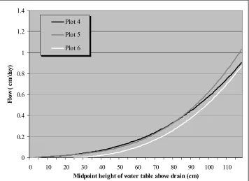
To demonstrate the change in hydrology that occurs when shallow drains are used
rather than deep drains, long term simulations were performed with the water management
model, DRAINMOD 5.1 (Skaggs, 1978). The simulations were conducted using weather
data from Plymouth, North Carolina collected from 1950 to 2000 and calibrated model inputs
for Plot 4 of the Tidewater Experiment Station research site described in detail in the
following section. Drain spacing for both simulations was 22.73 m. Drain depth for the deep
and shallow simulations were 1.50 and 0.75 m respectively. The soil was Portsmouth sandy
loam. Seepage was assumed to be negligible in both cases.
The results of the simulations are summarized in Table 1.1. Since the results for the
shallow and deep drain depth are predicted rather than measured values, their relationship
was described with percent difference, which is the difference of the values divided by the
average of the values. Average annual subsurface drainage from shallow drains was 34%
less than that from deep drains. Average annual surface runoff from the shallow drain
Figures 1.1 to 1.4 show the year to year variation of predicted water table depth, subsurface
drainage, surface runoff and ET respectively for the two drain depths.
The predicted changes in hydrology caused by reducing the drains depth, as shown in
Table 1.1 and Figures 1.1-1.4, favor a decrease in NO3-N losses. Use of shallow drains
decreases subsurface drainage, so, assuming concentrations are not substantially increased,
NO3-N losses should be reduced. A greater portion of the total outflow is surface runoff,
which has a low NO3-N concentration, compared to subsurface drainage. Increased
evapotranspiration reduces total outflow, and hence the loss of NO3-N. Additionally, the
higher water table resulting from the shallow drains should increase the thickness of the
reduced zone and promote denitrification (Skaggs and Chescheir, 2003).
Few studies have been done that examine the water quality effects of shallow drains
versus deep drains. Gordon and associates (1998) conducted a three year study in Onslow,
Nova Scotia, Canada evaluating nitrate-nitrogen losses from several drainage systems. The
drainage systems used included (i) 100 mm tile drains at 0.80 m depth and 12 m spacing (ii)
50 mm drains with 0.80 m depth and 12 m spacing and (iii) 50 mm drains at 0.50 m depth
and 12 meter spacing. The soil at the research site was classified as poorly drained. The
concentration of nitrate-nitrogen in the outflow from all drains was about 10 mg L-1. But,
0.5 m deep with 6 m spacing. Nitrate-nitrogen losses were 18.7 and 11.2 kg ha-1 for deep and
shallow subsurface drainage plots respectively. Shallow drains resulted in a reduction in
NO3-N loss of 50%, compared to the deep drains.
Skaggs and Chescheir (2003) conducted a simulation modeling study to examine the
effects of drain depth on nitrogen losses in drainage water. The simulations were performed
with DRAINMOD-N (Brevé, 1997) for continuous corn production using 40 years of
weather data from the Tidewater Research Station in Plymouth, NC. The soil was the very
poorly drained Portsmouth sandy loam. Simulations were performed for drain depths of
0.75, 1.00, 1.25, and 1.50 m. For each drain depth, simulations were conducted for drain
spacing between 5 and 300 m. For each drain depth, a spacing was selected that provided
maximum profit based on an economic analysis. The analysis considered the amortized cost
of drainage system, cost of corn production and expected profit from corn yield. Using the
optimum spacing for each depth, the predicted NO3-N loss ranged from 12 kg ha-1 for the
0.75 m depth to 31 kg ha-1 for a drain depth of 1.5 m.
Cooke et al. (2002) conducted a field study in East Central Illinois to determine the
effect of drain depth on hydrology and water quality. The experiment was conducted on
Drummer silt loam, which is described as poorly drained. Subsurface drains were installed at
the site specifically for this project. Drains were installed at (i) 0.61 m depth and 15.24 m
spacing, (ii) 0.91 m depth and 30.48 m spacing and (iii) 1.22 m and 30.48 m spacing. All
drain tubing was 101.4 mm in diameter. One year of data was collected. The researchers
amount of NO3-N lost in subsurface drainage, with less NO3-N lost from shallow than from
deep subsurface drains.
Burchell et al. (2003) conducted a field experiment near Plymouth, NC to examine
the effect of drain depth on nitrate-nitrogen loss in drainage water from a grazed field. The
field was irrigated with wastewater from a swine lagoon. Soil in the field was Cape Fear
loam, which is very poorly drained under natural conditions. Two drainage systems were
installed for the project. The shallow drains were placed at 0.75 m depth and 12.5 m spacing.
Deep drains were installed at 1.5 m depth and 25 m apart. Data were collected for 21 months.
During that time, total outflow from the shallow plots was significantly reduced relative to
deep plots. Nitrate-nitrogen loss from the shallow and deep plots was 35 and 42 kg ha-1
respectively for the 21 month period. However, the difference in nitrate export was not
statistically significant at the 10% level.
A field experiment was conducted at the Tidewater Research Station near Plymouth,
North Carolina. The objective of the experiment was to determine the effect of drain depth
on nitrate nitrogen loss in subsurface drainage water.
(Typic Umbraquult, fine-loamy over sandy of sandy skeletal, mixed, thermic), which under
natural conditions is very poorly drained. The predominant soil in Plot 6 is Cape Fear loam
(Typic Umbraquult, clayey, mixed, thermic), which is also very poorly drained under natural
conditions (Kleiss et al, 1993) (Figure 1.6). The field is surrounded on all sides by ditches
approximately 2.0 m deep (Munster, 1994). The subsurface drain lines used for this
experiment were installed prior to the design and implementation of this field experiment.
The site was cleared for agriculture in 1975. The original drainage system consisted
of parallel open ditches 85 m apart, about 1.2 m deep oriented north to south. A subsurface
drainage system was installed in 1985. Two out of three drainage ditches were filled and
corrugated plastic drain tubes were installed in the east-west direction (Skaggs, 2003). The
drains were 101-mm diameter and were installed 22.9 m apart and 0.8 to 1.0 m deep
(Munster, 1994).
The field was instrumented for research in 1988-1989 and was divided into eight
plots, each consisting of the area drained by three adjacent drains. A vault was buried at the
end of each plot to receive the drainage water from all three drainage lines. The
experimental system for the original drains is described in detail by Munster (1992). Flow
from the central drain line was measured and sampled for water quality. The outer lines
served to hydraulically isolate or “guard” the central line from the effects of adjacent plots.
A second set of drain lines was installed in 1991 at a depth of 1.2 to 1.3 m. The new drains
were placed midway between the old drains lines, and also have 22.9 m drain spacing.
For this experiment, the shallow (original) drain lines were used for Plots 1, 2 and 3.
The deeper drain lines were used in Plots 4, 5 and 6. On May 3, 2001 deep drain lines in
Plots 1, 2 and 3 were severed from the receiving vault and capped and the shallow drains
were opened. No changes were made in Plots 4, 5, and 6. Drainage system characteristics
are shown in Table 1.2. The average depths of the shallow and deep drains were 0.86 m and
1.20 m, respectively.
To achieve the objective of determining whether shallow drains reduce nitrate losses
compared to deeper drains, data collected between May 12, 2001 and December 31, 2002
were considered. On May 12, 2001, a large rainfall event occurred which raised the water
table to the surface, giving comparable initial conditions for all plots. Crops grown on the
site during the study were corn in 2001 followed by wheat and soybean in 2001/2002.
Management and cropping practices were typical of the region.
Data Collection
Precipitation, water table depth and subsurface drainage volume were measured and
continuously recorded. Subsurface drainage was sampled using a flow-proportional sampler
30 minutes. The micrologger received data from a variety of devices, which were mounted
on a 4.57 m (15 ft) tripod. The devices included a Campbell Scientific (CSI)-107B sensor to
measure soil temperature, a Met 101B sensor to measure air temperature, a Met
One-HMP45C sensor to measure relative humidity, a Met One-024A sensor to measure wind
direction, a Met One-014A to measure wind speed, Licor-LI200X sensor to measure total
solar radiation, and a Radiation and Balance Systems-Q7.1 sensor to measure net solar
radiation. Rainfall was measured with a tipping bucket rain gage manufactured by Texas
Electronics (TE525).
Rainfall was also measured with a second tipping bucket rain gage near the
instrument house at plot 1. This device triggered a HOBO data logger on every tip,
representing 0.254 mm of rain. Additionally, rainfall was measured with a manual gage.
The three measurements were then compared to check for accuracy, consistency and
completeness of record.
Water Table Depth
Two water table recorders are located at the quarter points, north and south of the
shallow central drain line, in each plot. Water table depth was measured with a float and
pulley system connected to a potentiometer (Figure 1.9). Output voltage from the
potentiometer was recorded every thirty minutes with a 4 channel HOBO data logger. In
addition, a chart recorder on the north well in each plot gave a visual record of water table
It was necessary to convert the voltages recorded by the data logger into depth
measurements. To do this, a linear function was developed, with depth as the independent
variable and voltage as the dependent variable. The slope of the function was the diameter of
the pulley connected to the float. The intercept value was found by matching the computed
value of depth at the time of data download with the actual depth read in the field at the same
time. Typically this value remained constant. It did change occasionally, such as when the
equipment was disturbed by an animal.
Subsurface Drainage
All subsurface drain lines outlet to cylindrical PVC tanks (0.61 m in diameter and 1.8
m in height), which are located in large underground vaults covered by an instrument house
(Figure 1.11). Measurements were conducted and drainage water was sampled for water
quality on the center drainage line which emptied into a separate tank. The drain lines on
either side of the center line, “guard” lines, emptied into the “guard” tank, which has the
same dimensions as the center line tank (0.61 m diameter, 1.83 m in height).
Subsurface flow rate was measured by two systems (Figure 1.12). In the first system,
the depth of water in the center line tank was monitored. The level was measured with a
in set points multiplied by the cross sectional area of the tank. Since water flow into the tank
did not stop during pumping, a method to account for inflow during the pumping cycle was
used. During very high inflow, the pump ran continuously and the number of pump cycles
was not representative of the amount of water pumped from the center line tank. For this
situation, the second method of flow measurement was used. The potentiometer method was
also used to record the flow volume from the guard drain lines.
A Signet® Industrial MK515 Paddlewheel Flowmeter was connected to the outflow
pipe from the center line tank as a second method of measurement. As water was pumped
from the centerline tank, it passed through the paddle portion of the flowmeter. Each
revolution of the paddlewheel represented a fixed volume of water. The number of
revolutions was recorded with a Blue Earth microprocessor. Flow was proportional to the
number of revolutions. Output from the microprocessor was a flow volume calculated by
multiplying the number of revolutions times a fixed volume of water, which was determined
by calibration. During times of high flow, this method of measurement was preferable since
it was not dependent on pump cycles to measure flow.
Both the potentiometer method and the paddlewheel meter provided measurements of
flow timing and volume. A Precision PMM 5/8” Water Meter®, connected in series with the
paddlewheel meter on the outflow pipe from the center line tank, was used to determine to
total volume leaving the system. This “master” meter was read biweekly when data were
downloaded from the Blue Earth computer. These measurements were used to determine the
Equipment failure occurred on occasion during high flow events. In particular, the
equipment in plots 2 and 4 were damaged during a large storm on August 30, 2002 and
drainage amounts for this event were approximated from the data that was recorded and the
relationship between these plots (2 and 4) and the other plots.
During February of 2003, the “master” meter on plot 2 became clogged and did not
capture the actual flow amount through the system for a two week period. Data from the
potentiometer was used to determine flow timing and relative flow rates. The volume was
determined by scaling the hourly potentiometer data by a factor based on historical
relationship between the main meter and the potentiometer.
The remainder of the time, any equipment failure corresponded to power loss which
did not allow the sump pumps to evacuate water from the control tank as it came in. This
caused water to back up in the profile until the breaker was reset. The profile then drained to
equilibrium in relatively short time. Power failures occurred on three occasions in Year 1
and twice in Year 2. In each case, power was restored within 24 hours.
The master meters in each house were calibrated twice during the course of the study.
The first test was conducted after the master meters were removed and brought into the
laboratory for testing on January 30, 2002. The second testing occurred November 24, 2003.
Water Quality Analysis
Subsurface drainage water was sampled from the outflow pipe of the center line tank.
A 12-mm diameter flexible tube was affixed to the outflow line; each time the sump pump
removed water from the control tank, approximately 0.5% of the water was diverted to a
water quality sampling container. The flexible tube entered through the side of a refrigerator
located in the instrument house and emptied into a 20 L container. A composite sample was
allowed to accumulate for 2 weeks. Then the water was mixed and placed in a 500 mL
Nalgene sample bottle and placed in a freezer until transport to the Water Quality Laboratory
in the Soil Science Department at North Carolina State University.
Subsurface drainage samples were analyzed for nitrate (NO3-N), ammonium (NH4
-N), total Kjeldahl nitrogen (TK-N), orthophosphate (PO4), total phosphorus (TP) and chloride
(Cl-) by standard methods (APHA, 1995). Testing for NO
3-N, NH4-N, orthophosphate, and
total phosphorus were performed with a Quickchem 8000 Automatic Ion Analyzer. Analysis
for NO3--N, ammonium and orthophosphate, was conducted on a single sample, which was
first filtered through a 0.45µm filter. Nitrate was analyzed using the cadmium reduction
method. Ammonium was analyzed by the salicylate method. Orthophosphate was analyzed
by the ascorbic acid method. Total Kjeldahl nitrogen was analyzed using the Kjeltec System
1026 Distilling Unit.
Cropping and Fertilization
harvested June 11, 2002. Soybean was planted June 18, 2002 and harvested November 26,
2002. Planting, nutrient and pesticide management practices were typical of the region.
Prior to the planting of corn in 2001, lime was applied to plot one only on March 30.
The total amount of nitrogen applied to the corn was 170.8 kg N ha-1. Of that amount, 25.3
kg N ha-1 was added on March 30, 2001. Side dress applications of urea ammonium nitrate
were added on April 20, 2001 and June 2, 2001 at a rate of 72.8 kg N ha-1. November 13,
2001, prior to the wheat planting, nitrogen was applied to all plots at a rate of 25.3 kg ha-1.
Urea ammonium nitrate was applied as a side dress application at a rate of 90.9 kg N ha-1to
all plots on March 11, 2002. Cropping sequence and fertilizer applications are summarized in
Table 1.3.
RESULTS AND DISCUSSION
The objective of the study was to determine whether NO3-N losses from shallow
subsurface drains would be significantly different than losses from deeper drains. The field
study was conducted near Plymouth, NC from May 12, 2001 to April 30, 2003. The period
May 12, 2001 to April 30, 2002 is referred to as Year 1, and the period May 1, 2002 to April
during 2002. No problems occurred with the manual gage or the CR10 tipping bucket gage.
The R2 tipping bucket became clogged and did not record rainfall between April 2, 2002 and
May 18, 2002. The problem was repaired in mid-May of 2002. Cumulative precipitation
recorded by the manual gage, CR10 tipping bucket and R2 tipping bucket for Year 1 was
1016 mm, 958 mm and 763 mm respectively (Figure 1.13). The totals for Year 2 were 1383
mm, 1356 mm, and1238 mm (Figure 1.14). For the study period, the CR10 tipping bucket
rain gage performed well consistently. The precipitation measured with this device was
assumed to best represent the timing and amount of actual precipitation. These data, as well
the long term cumulative monthly average precipitations, are presented by monthly totals in
Table 1.4.
A comparison of Year 1 and Year 2 measured monthly precipitation to the long term
average monthly values (based on the period 8/19/1948 to 12/31/2000) (Figure 1.15)
indicates prolonged periods of significantly below average rainfall during the study period.
Observed rainfall for the months August 2001 through December 2001 was 354 mm below
the long term average (178 mm compared to 532 mm). For those months of drought
conditions, drainage outflow was substantially below average.
A second period of low rainfall occurred from April 2002 through June 2002.
Measured rainfall was 178 mm as compared to long term average rainfall for the same
months of 320 mm. Again, drainage outflow was greatly reduced during this period. Yet,
considering the calendar year of 2002, yearly precipitation looks to be nearly normal with the
prolonged periods without rainfall, the water table fell below the lower limit of the
monitoring well. When this occurred the water table elevation appears as a straight line.
This occurred during the summers of 2001 and 2002. Variation in water table depth is seen
from plot to plot. Average water table depth for each plot, based on quarterly periods, is
shown in Table 1.5.
Despite the fact that the soil type in the shallow drain plots (plots 1, 2 and 3) is the
same and the drain depths in these plots are nearly identical (0.86, 0.85 and 0.87 m),
considerable variation is seen in the daily water table depths. On a quarterly basis, the water
table for plot 1 was the shallowest of all plots. For the entire study period, plot 1 was, on
average, 70 mm closer to the surface than plot 3 and 100 mm closer to the surface than plot
2. The water table in plot 2 was consistently the deepest of the shallow drains. For the two
year period the average water table depths for plots 1, 2 , and 3 were 0.63, 0.75, and 0.70 m,
respectively.
The drain depths for the deep plots (plots 4, 5, and 6) are similar: 1.22, 1.18, and 1.20
m respectively. However the soil type in plot 6 (Cape Fear Loam) is different than the soil
type in plots 4 and 5 (Portsmouth Sandy Loam). Generally, the water table elevation in plots
4 and 5 were very similar. The water table response in plot 6 differs from 4 and 5. For a
Examination of Figures 1.16-1.20 indicates that water table depths in plots 1-3 are
generally less than in plots 4-6. Plot 6 is frequently an exception, but this could also be
expected because the Cape Fear soil in plot 6 has lower hydraulic conductivity than the
Portsmouth soil in the other plots. Plot 2 also appears to be an exception during some
periods with the water table falling to or below those measured in plot 5 (e.g. Figure 1.16).
Water table response for plot 2 appears to be more of an exception to the expected trends
during the wettest periods (Figures 1.22 and 1.23). When water tables from all plots were
less than 60 cm deep for extended periods (Figures 1.22 and 1.23) the water table in plot 2
was as deep or deeper than those for plots 4-6.
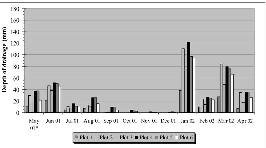
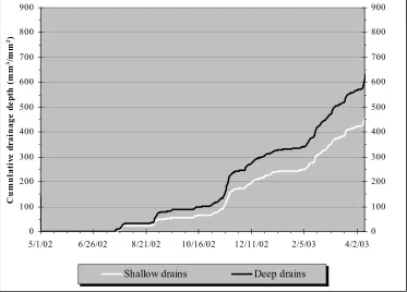
Subsurface drainage measurements are shown in Figure 1.24 to Figure 1.27. Figures
1.24 and 1.25 present the cumulative drainage from each plot for Years 1 and 2.
Figures 1.26 and 1.27 show monthly drainage volumes (in units of depth; i.e. cm3 per cm2 of
surface area) from each plot for Years 1 and 2, respectively. Numerical values of monthly
flow are presented in Table 1.6.
There was considerable variation in drainage flows, both temporally and from
plot-to-plot. In Year 1, precipitation was significantly below average (Table 1.4), water tables were
relatively deep, and flow rates were low. During the summer months, evapotranspiration
exceeded rainfall and water table levels dropped below the drain depth for all plots. As
expected, no flow was observed when water table levels fell below the drain. Except for plot
2, cumulative drainage from all plots in Year 1 conformed to the expectation that more water
shallow drains and was more than plot 6, a deep drain, but in a slowly permeable (tighter)
soil, as mentioned earlier.
In Year 2 of the study, after below average rainfall in May and June, rainfall amounts
were equal or greater than normal for the remainder of the year, and subsurface drainage
volumes increased relative to Year 1. Once again, subsurface drainage from Plot 2 was
greater than expected. Flow from plot 2 was actually greater than all other plots during Year
2.
For the entire study period, Plot 2 had the greatest amount of drainage, followed by
Plot 4, Plot 5, Plot 6, Plot 3, and Plot 1, in order of decreasing magnitude. An analysis of
variance on monthly drainage flows showed no significant difference between the shallow
and deep drains at the 10% level. The lack of significant difference in drainage outflows was
mostly due to much higher than expected drainage from plot 2.
There are several possibilities for explaining the unexpected wide variability in
drainage volume among the three plots with shallow drains. It appears that the three plots
were not operating as hydraulically isolated units. An examination of the monthly drainage
from the three plots (Table 1.6, Figure 1.26 and 1.27) indicates interaction between plots 1
and 2. Drainage from plot 1 was less than half of that from plot 2 in nearly every month.
and/or plot 3. The biggest differences in monthly drainage flows from the three plots
occurred when the water table was at or close to the surface during January and March 2002
(Figures 1.19 and 1.26) and November 2002 through April 2003 (Figures 1.22, 1.23 and
1.27).
For this scenario, consider the monthly flow from Plot 3 as ‘normal’. Then subtract
the amount of flow in excess of ‘normal’ from the Plot 2 amount and add it to the Plot 1
amount. The result would be nearly identical outflow for each shallow drain, the expected
result.
The water table plots (Figure 1.19, 1.22 and 1.23) for these periods show that water
was frequently ponded on the surface of plot 1 and to a lesser extent on plot 3, but not on plot
2. Rather than leaving the field, runoff from plot 1 and possibly plot 3, could have flowed to
plot 2 where it infiltrated and increased drainage flows compared to the other plots.
Other information suggests the possibility of subsurface flow from Plot 1 to Plot 2.
Figure 1.28 graphically depicts the soil layering and corresponding conductivities in the field.
The layering and lateral saturated hydraulic conductivity values were reported by
Mohammad (1997). During this study, water table levels in plot 1 were, on average, 100 mm
closer to the surface than plot 2. Also, water table levels in plot 3 were, on average 30 mm
closer to the surface than plot 2. This indicates a hydraulic gradient between the plots. Also,
the lateral saturated hydraulic conductivities in plot 1 are lower than plot 2 for all layers of
the profile. The drain in plot 1 is at an interface of two layers. The layer above has
hydraulic head losses as the water flows to the drain would be smaller and flow rates greater
in plot 2 than in plot 1. Differences in the hydraulic conductivity of the soil surrounding the
drain could have resulted in the higher water tables and slower drainage from plot 1 as
compared to plot 2. This could have caused the surface runoff and shallow subsurface flow
from plots 1 and 3 to plot 2 as discussed above. Another possible cause of reduced flow in
plot 1 is blockage of the drains by physical obstructions such as plant roots or sediment or
sealing of the holes in the drains by soil particles or ochre (Ford, 1979) This would reduce
flows, raise the water table and cause the effects discussed above for the interaction of plots 1
and 2.
If a lack of independence is assumed within treatments, an option for considering the
effect made by the difference in drain depth is to combine the total flow for each treatment
and examine the average depth of drainage for each treatment. Average flow from the
shallow drains, relative to the flow for the deep drains was reduced 35% for Year 1 (Figure
1.29) and 26% for Year 2 (Figure 1.30).
The specific cause of the interaction between plots can not be stated until further
investigation is conducted. However, it can be said that each shallow plot responds quite
differently, while each deep plot responds similarly. To illustrate drainage response in each
and ET was low. Therefore, data were included in the sample only for the months December
through March. Data were excluded during that period if daily rainfall exceeded 4.5 mm, if
rainfall the previous day exceeded 20 mm.
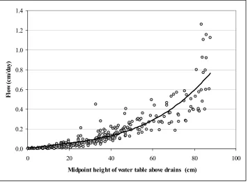
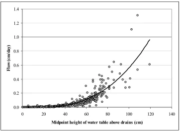
Certainly similarities can be seen in the graphs for each plot. As would be expected,
when the midpoint height of the water table is near zero, flow is near zero. Also, for any
particular water table elevation, a range of flow rates can be expected. This occurs because
for a particular value of midpoint water table height, many water table profiles are possible.
The possibilities vary from a relatively flat water table profile, if ponded conditions exist or if
ET is high, to the elliptical shape found when the elevation of water directly above the drains
is zero (i.e., when the water table intersects the drains). Any intermediate shape is possible.
The greater the height of water table above the drains the greater the flow rate. For the
shallow plots, there were large differences in the relationship between flow rate and water
table elevation from plot to plot. For a given water table height, daily flow from plot 2 is
more than twice that from plot 1 and about 1.5 times more than from plot 3. Even when the
water table height is small, significant flow was measured in plot 2. Results in Figure 1.31
for plot 1 are consistent with earlier speculation of partial blockage or sealing of the drain.
Unlike the other plots, measured flow rates were zero until the water table elevation
exceeded 0.2 to 0.3 m.
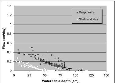
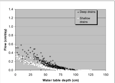
Since this field has been instrumented and monitored continuously during the recent
past, it is possible to compare the behavior of the shallow drains in Plots 1, 2 and 3 with the
1.41, water table depth is plotted against drainage rate for plots 1, 2 and 3. In general, for the
same water table depth, higher flow rates are expected from deep drains than from shallow
drains due to greater hydraulic head. This behavior is clearly observed in Plots 1 and 3.
However, in Plot 2 this was not the case for all water table depths. For water table depths
less than 0.4 m, higher flow rates were observed for the shallow drains, than for the deep
drains. It is likely that flow is higher because of a reduction of convergence head losses at
the drain. The shallow drain is in a layer with lateral saturated hydraulic conductivity of 2.04
cm hr -1. The deep drain in Plot 2 is in a layer with conductivity of 0.47 cm hr -1. Clearly,
field variability will affect the behavior of the drainage system.
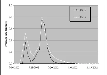
The response of water table and drainage rates for individual storm events, illustrates
the effect of drain depth on hydrology of drained fields. Results are given in Figures
1.42-1.45 for two storm events. Results for storm event 1 illustrates that drainage continues to
flow from deep drains after it has stopped from shallow drains. Prior to the first storm event,
water table depths in both plots 3 (shallow drains) and 4 (deep drains) were greater than 1.20
m. Rainfall in mid July continued periodically for nine days, during which time, 120 mm of
precipitation occurred. Water tables rose in both plots reaching a maximum elevation 5 cm
from the surface in plot 3 and 20 cm from the surface in plot 4 on July 26. Rainfall was
depth. The total amount drained during this period was 27 and 41 mm from Plots 3 and 4,
respectively.
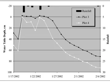
The second storm event illustrates the effect of drain depth on the proportion of total
outflow that leaves the plot as of surface or subsurface drainage. Prior to this event, the
deeper drains in plot 4 caused the water table depth to be greater at 0.61 m than in plot 3
where it was 0.40 m. Starting on January 19, 2002, precipitation of 56 mm fell over a seven
day period. The 30 mm of rainfall on January 19 caused the water table in plot 3 to rise
above the surface where it remained ponded for most of the next 7 days (Figure 1.44). The
ponded surface water was available for surface runoff, which, although not measured, almost
certainly occurred. In contrast, the greater amount of storage available in the profile, prior to
the event, prevented the water from ponding on the surface of plot 4. The water table nearly
rose to the surface, but then receded in response to more rapid drainage (compared to plot 3)
provided by the deeper drains (Figure 1.45). Consequently, no surface runoff occurred from
Plot 4 during this time. During the period of January 17, 2002 to February 5, 2002,
subsurface drainage from Plots 3 and 4 was 41 and 73 mm respectively. Thus the plots with
shallow drains lose a larger proportion of their total outflow by surface runoff and a smaller
proportion by subsurface flow compared to the plots with deeper drains.
Nitrogen
To determine nitrate-nitrogen losses in subsurface drainage, flow proportional
nitrate that had passed through the drain. Nitrate-nitrogen amounts lost from each plot
through subsurface drainage are given in Table 1.8. Average flow-weighted NO3-N
concentrations for the two year period were calculated for each plot (Table 1.9). The values
from plots 1-6 were 8.0, 7.1, 6.2, 5.9, 5.8, and 6.3 respectively. Analysis of variance was
used to compare NO3-N concentrations from shallow drain plots to deep drain plots. Some
variability in concentration occurred when individual samples were considered. However, at
the 10% level, there was no significant difference in average flow –weighted NO3-N
concentration from the shallow and deep drains.
Nitrate concentrations in drainage water ranged from 0.6 mg L-1 to 30.8 mg L-1 in the
shallow plots and from 0.4 mg L-1 to 17.4 mg L-1 in the deep plots. The highest
concentrations were seen following three applications of nitrogen based fertilizer to the 2001
corn crop. The highest concentrations were observed in Plots 1 and 3, the drains with the
lowest flow rates during this period. Despite the application of fertilizer and the high
concentrations in the drainage outflow, relatively little mass of nitrate nitrogen was lost
during this period because precipitation was low and very little water was being removed
from the profile via subsurface drainage. The drought persisted through the end of 2001,
water tables remained below the drain depth, little subsurface flow was seen and any
concentrations in Plots 3 through 6 were fairly consistent. Concentrations in plot 1 were
highest, followed by plot 2. The high concentrations seen in plot 1 were consistent with low
flow, but nitrate concentrations in plot 2 were high also. This suggests that NO3-N may have
been carried via lateral flow from plot 1 to plot 2.
Another long period of no flow or low flow occurred between May 2002 and
November 2002. Very little nitrate was exported during this time. Beginning in November
2002, precipitation fell regularly through the end of the study (April 30, 2003) generating
consistent subsurface drainage and nutrient export. During this time, the previously seen
trends continued. Nitrate nitrogen losses from Plot 2 were highest, followed by Plot 4, Plot
5, Plot6 Plot 3 and finally Plot 1.
Cumulative nitrate losses from each drain are shown in Figures 1.46 and 1.47 for
Years 1 and 2 respectively. For the shallow drains, plots 1, 2, and 3, the total amounts of
NO3-N lost in drainage water were 32.1, 82.5., and 37.3 kg NO3-N/ha. For the deep drains,
plots 4, 5, and 6, the total amount of NO3-N was 55.5, 52.6., and 46.2 kg NO3-N/ha. Results
of an analysis of variance on the total nitrate-nitrogen losses from three replications of two
treatments indicate that there is no significant difference at the 10% significance level
between the treatments.
As with the flow, average values of nitrate-nitrogen losses from shallow and deep
drains were calculated. Cumulative average nitrate-nitrogen losses from the shallow and
deep drains are shown in Figures 1.48 and 1.49. During Year 1, the average loss from the
deep drains (23.5 kg ha-1). The net result was nearly equal nitrate nitrogen losses from the
shallow drains (50.6 kg ha-1) and the deep drains (51.5 kg ha-1).
SUMMARY AND CONCLUSION
A field study was conducted in the Lower Coastal Plain of North Carolina to
determine whether shallow subsurface drains would reduce nitrate nitrogen losses in drainage
effluent relative to deep subsurface drains. The field study was conducted over a two year
period between May 12, 2001 and April 30, 2003. The experimental site was a 13.8 ha
agricultural field at the Tidewater Research Station, near Plymouth, North Carolina. The site
was nearly flat and the soils were classified as Portsmouth and Cape Fear sandy loams, both
very poorly drained under natural conditions. The site was subdivided into eight 1.8 ha plots,
with three parallel drains per plot. Plots one through three were drained with parallel drains
at an average drain depth of 0.86 m. Plots four through six were drained with deeper parallel
drains, with an average depth of 1.20 m. Plots seven and eight were not used in this study.
The crop was a corn-wheat-soybean-crop rotation.
Precipitation, water table depth and subsurface drainage were measured continuously.
Precipitation was measured with tipping buckets at two locations on the site and with a
The hypothesis was that water tables would remain higher in the shallow plots than
the deep plots, outflows from the shallow drains would be significantly less than from the
deep drains, and nitrate losses from the shallow drains would be significantly less than from
the deep drains.
Average water table depths in the shallow drain plots were 0.63, 0.75, and 0.70 m for
plots 1-3, respectively. Average water table depths in the deep drain plots were 0.81, 0.78,
and 0.78 m for plots 4-6, respectively. Analysis of variance was used to determine that the
average water table depth in the shallow drain plots was significantly less than the average
water table depth in the deep drain plots, at the 10% level.
In Year 1, the average flow from the shallow drains and deep drains was 236 mm and
364 mm respectively, a reduction of 37%. In Year 2, the average flow from the shallow
drains and deep drains was 499 mm and 674 mm respectively, a reduction of 26%. The
reason the differences were not significant was apparent interaction between plots 1 and 2
and perhaps 3.
There was no significant difference in NO3-N losses from the shallow and deep
subsurface drains. Differences were confounded by interaction among shallow drains and to
Table 1.1. Average annual results from 50-year DRAINMOD simulation comparing deep and shallow subsurface drains using meteorological data collected at Tidewater Research.Station, Plymouth, NC.
Deep drains Shallow drains % diff
(cm) (cm)
Subsurface drainage 52.3 37.1 33.8
Surface runoff 9.9 18.6 -60.9
Evapotranspiration 67.3 73.7 -9.1
Infiltration 119.6 110.9 7.6
Water Table Depth 102 69.6 37.8
Table 1.2. Drainage system characteristics of experimental plots from research site at Tidewater Research Station, Plymouth, North Carolina.
Plot 1 Plot 2 Plot 3 Plot 4 Plot 5 Plot 6 Subsurface Drainage
Drain Spacing (cm) 2284 2272 2276 2273 2285 2294
Drain Depth (cm) 86 85 87 122 118 120
Effective Drain Radius (cm) 1 1 1 1 1 1
Drainage coefficient (cm/day) 0.6 1.5 1.5 1.5 1.5 1.5 Depth to impermeable layer(cm) 240 240 240 240 240 240 Surface Drainage
Maximum, surface storage (cm) 0.3 1.5 0.5 1 1.4 1.5
Kirkham's depth (cm) 0.15 0.75 0.25 0.5 0.7 0.75
Table 1.3. Cropping and fertilization schedule during drain depth experiment.
Lime Nitrogen Fertilizater
Crop Date Activity Application Application