Manufacturing Systems Line Balancing using Max-Plus Algebra

(1)

University of Windsor University of Windsor

Scholarship at UWindsor

Electronic Theses and Dissertations Theses, Dissertations, and Major Papers

9-26-2018

Manufacturing Systems Line Balancing using Max-Plus Algebra

Ali Fakhri

University of Windsor

Follow this and additional works at: https://scholar.uwindsor.ca/etd

Recommended Citation Recommended Citation

Fakhri, Ali, "Manufacturing Systems Line Balancing using Max-Plus Algebra" (2018). Electronic Theses and Dissertations. 7518.

https://scholar.uwindsor.ca/etd/7518

This online database contains the full-text of PhD dissertations and Masters’ theses of University of Windsor students from 1954 forward. These documents are made available for personal study and research purposes only, in accordance with the Canadian Copyright Act and the Creative Commons license—CC BY-NC-ND (Attribution, Non-Commercial, No Derivative Works). Under this license, works must always be attributed to the copyright holder (original author), cannot be used for any commercial purposes, and may not be altered. Any other use would require the permission of the copyright holder. Students may inquire about withdrawing their dissertation and/or thesis from this database. For additional inquiries, please contact the repository administrator via email

(2)

Manufacturing Systems Line Balancing using Max-Plus Algebra

By

Ali Fakhri

A Thesis

Submitted to the Faculty of Graduate Studies

through the Industrial Engineering Graduate Program

in Partial Fulfillment of the Requirements for

the Degree of Master of Applied Science

at the University of Windsor

Windsor, Ontario, Canada

(3)

ii

Manufacturing Systems Line Balancing using Max-Plus Algebra

By

Ali Fakhri

APPROVED BY:

______________________________________________ R. Caron

Department of Mathematics and Statistics

______________________________________________ W. ElMaraghy

Department of Mechanical, Automotive and Materials Engineering

______________________________________________ H. ElMaraghy, Advisor

Department of Mechanical, Automotive and Materials Engineering

(4)

iii

DECLARATION OF ORIGINALITY

I hereby certify that I am the sole author of this thesis and that no part of this thesis has been published or submitted for publication.

I certify that, to the best of my knowledge, my thesis does not infringe upon anyone’s copyright nor violate any proprietary rights and that any ideas, techniques, quotations, or any other material from the work of other people included in my thesis, published or otherwise, are fully acknowledged in accordance with the standard referencing practices. Furthermore, to the extent that I have included copyrighted material that surpasses the bounds of fair dealing within the meaning of the Canada Copyright Act, I certify that I have obtained a written permission from the copyright owner(s) to include such material(s) in my thesis and have included copies of such copyright clearances to my appendix.

(5)

iv ABSTRACT

In today's dynamic environment, particularly the manufacturing sector, the necessity of being agile, and flexible is far greater than before. Decision makers should be equipped with effective tools, methods, and information to respond to the market's rapid changes. Modelling a manufacturing system provides unique insight into its behavior and allows simulating all crucial elements that have a role in the system performance.

Max-Plus Algebra is a mathematical tool that can model a Discrete Event Dynamic System in the form of linear equations. Whereas Max-Plus Algebra was introduced after the 1980s, the number of studies regarding this tool and its applications is fewer than regarding Petri Nets, Automata, Markov process, Discrete Even Simulation and Queuing models. Consequently, Max-Plus Algebra needs to be applied and tested in many systems in order to explore hidden aspects of its function and capabilities.

To work effectively; the production/assembly line should be balanced. Line balancing is one of the manufacturing functions that tries to divide work equally across the production flow. Car Headlight Manufacturing Line as a Discrete Manufacturing System is considered which is a combination of manufacturing and assembly lines composed of different stations. Seven system scenarios were modeled and analyzed using Max-Plus to balance the car headlights production line. Key Performance Indicators (KPIs) are used to compare the various scenarios including Cycle Time, Average Deliver Rate, Total Processing Lead Time, Stations' Utilization Rate, Idle Time, Efficiency, and Financial Analysis. FlexSim simulation software is used to validate the Max-Plus models results and its advantages and drawbacks compared with Max-Plus Algebra.

This study is a unique application of Max-Plus Algebra in line balancing of a manufacturing system. Moreover, the problem size of the considered model is at least twice (12 stations) that of previous studies. In the matter of complexity, seven different scenarios are developed through the combination of parallel stations and buffers. Due to that the last scenario is included four parallel stations plus two buffers

(6)

v

DEDICATION

I would like to express my deep gratitude to my wife who helped me and supported my

(7)

vi

ACKNOWLEDGMENTS

Before all, praise goes to God for giving me the strength and knowledge to complete this work. The completion of this dissertation would not have been possible without the support and help of many people, to whom I would like to express my gratitude. On top of the list comes Dr. Hoda ElMaraghy, my supervisor, who provided me with continuous and invaluable support, guidance, and mentorship. I would also like to express my appreciation to the Ph.D. committee members: Dr. Richard Caron and Dr. Waguih ElMaraghy for their valuable comments and suggestions that vastly improved the quality of this thesis. Special thanks also go to my colleagues and mentors at the Intelligent Manufacturing Systems (IMS) Centre at the University of Windsor.

(8)

vii

TABLE OF CONTENTS

DECLARATION OF ORIGINALITY iii

ABSTRACT iv

DEDICATION v

ACKNOWLEDGMENTS vi

LIST OF TABLES x

LIST OF FIGURES xi

LIST OF ABBREVIATIONS AND NOTATION xiii

CHAPTER ONE: INTRODUCTION 1

1.1.Motivations 1

1.2.System Attributes ₁

1.3.Classifications of Discrete Event System (DES) ₃ 1.4.Discrete Event Systems Modelling Methods (Formal Methods) 4

1.5.Max-Plus Algebra 7

1.6.Advantages and Drawbacks of Max-Plus Algebra 13

1.7.Gap Analysis 15

1.8.Research Scope 16

1.9.Research Contributions 17

1.10. Thesis Statement 18

1.11. Research Overview 18

CHAPTER TWO: BASIC OF MAX-PLUS ALGEBRA AND MATHEMATICAL

CONCEPTS 19

2.1.Introduction 19

2.2.Max-Plus Algebra 19

2.3.Max-Plus Algebra over Matrices 19

2.4.Modelling a Manufacturing system using Max-Plus Algebra 20

(9)

viii

CHAPTER THREE: MODELLING OF MANUFACTURING SYSTEM BY

MAX-PLUS ALGEBRA 23

3.1.Introduction 23

3.2.The General Proposition of a Model using Max-Plus Algebra 23

3.3.Modelling of a Manufacturing System 24

3.4.The General form of Modelling Formulation using Max-Plus Algebra 28

3.5.Summary 32

CHAPTER FOUR: CAR HEADLIGHT MODELLING AND LINE BALANCING BY 33

4.1. Introduction 33

4.2. Car Headlight Manufacturing System 33

4.3. Line Balancing Scenarios 39

4.4. Analysis and Results 47

4.5. Summary 56

CHAPTER FIVE: DISCRETE EVENT SIMULATION (FLEXSIM) 58

5.1.Introduction 58

5.2.FlexSim as a Discrete Event Simulation tool 58

5.3.Analysis 58

5.4.Comparison Max-Plus Algebra with FlexSim 80

5.5.Summary 81

CHAPTER SIX: DISCUSSION AND OVERVIEW 82

6.1.Discussion and Overview 82

6.2.Novelties and Contributions 84

6.3.Limitations 84

6.4.Recommendations for Future Studies 85

REFERENCES 86

APPENDIX ONE 92

APPENDIX TWO 96

(10)

ix

APPENDIX FOUR 102

(11)

x

LIST OF TABLES

Table 1-1 Max-Plus Algebra Developed Theories 9

Table 1-2 Max-Plus Algebra Application 12

Table 1-3 Max-Plus Algebra Industrial Applications 13 Table 4-1 List of Car Headlight Parts and Components 35 Table 4-2 Process Plan Car Headlight Manufacturing Line 37 Table 4-3 General Findings of system modelling 49

Table 4-4: Financial Analysis 55

Table 5-1 the FlexSim data transferred into the Excel for scenario 7 59

Table 5-2 the required time needed to solve scenarios using Max-Plus Algebra 60

Table 5-1 FlexSim Data Transferred into The Excel for Scenario 1 68

Table 5-2 KPIs Outputs for Scenario 1 Obtained by Max-Plus Model 69

Table 5-4 KPIs Outputs for Scenario 2 Obtained By Max-Plus Model 62

Table 5-15 Total completion time (sec) at stations M and T 80

(12)

xi

LIST OF FIGURES

Figure 1.1 A General Modelling Process Structure 2

Figure 1.2 Major Systems Classification 3

Figure 1.3 Simple Petri Net Model 5

Figure 1.4 Simple Example of Automata Model 5

Figure 2.1 A mixed manufacturing system 21

Figure 3.1 A simple structure of a system 23

Figure 3.2 n series stations 25

Figure 3.3 "n" merged stations 26

Figure 3.4 Flow line with the parallel identical station 26

Figure 3.5 Flow line with the buffer station 27

Figure 3.6 An integrated model (Series, Merged, Parallel Stations and, Finite Buffer) 28

Figure 3.7 The General Structure of Car Headlight as a manufacturing system 28

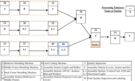
Figure 4.1 Scenario 1, The General Structure of modelled manufacturing system 34

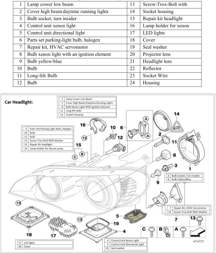
Figure 4.2 An exploded view of Car Headlight 35

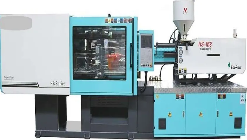
Figure 4.3 Molding Injection Machine 36

Figure 4.4 Laser Cutting Machine 36

Figure 4.5 Reflector Sub-Assembly Station into Lamp Seat 38

Figure 4.6 Projector Lens and Headlight Lens Holder Sub-Assembly Station 38

Figure 4.7 Plasma Spray and Adhesive Gluing 39

Figure 4.8 Air Tightness Test (Quality Inspection) 39

Figure 4.9 The Structure of Scenario 2, Parallel Identical Station 40

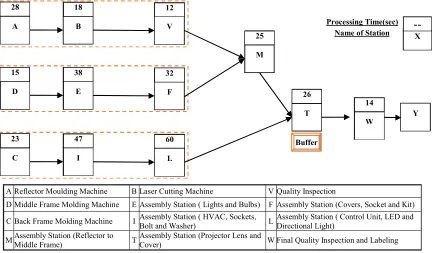
Figure 4.10 Structure of Scenario 3, Buffer at Station T 42

Figure 4.11 Structure of Scenario 4, Combination of Parallel Identical Station and Buffer 43

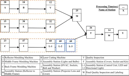
Figure 4.12 Structure of Scenario 5 Three Parallel Identical Stations 44

Figure 4.13 Structure of Scenario 6 Two Parallel Identical Station at I and L 45

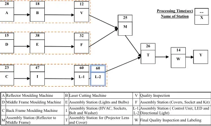
Figure 4.14 Structure of Scenario 7 the Combination of Four Parallel Identical Station and 46

(13)

xii

Figure 4.16 Capability of system to deliver a finished part by second 50

Figure 4.17 Total Processing Lead Time of Scenarios (Sec) for 30 parts 51

Figure 4.18 Average Utilization Rate of different scenarios 52

Figure 4.19 Efficiency and Idle Time of Scenarios 54

Figure 4.20 The Cost of Finished Part in Scenario ($) 56

Figure 5.1 Final Results for Scenario 1 60

Figure 5.2 FlexSim Gantt Chart for Scenario 1 61

Figure 5.3 Final Results for Scenario 2, Two Parallel Stations at L 63

Figure 5.4 FlexSim Gantt Chart for Scenario 2, two Parallel stations at L 64

Figure 5.5 Final Results for Scenario 3, Buffer at Station T 66

Figure 5.6 FlexSim Gantt Chart for Scenario 3, Buffer at Station T 67

Figure 5.7 Final Results for Scenario 4, Two Parallel Station at L and Buffer T 69

Figure 5.8 FlexSim Gantt Chart for Scenario 4, two Parallel station at L and Buffer T 70

Figure 5.9 FlexSim Cycle Time for Scenario 5, Three parallel stations at L 72

Figure 5.10 FlexSim Gantt Chart for Scenario 5, Three parallel stations at L 73

Figure 5.11 FlexSim cycle time for Scenario 6, Two Parallel Stations at I and L 75

Figure 5.12 FlexSim Gantt Chart for Scenario 6, Two Parallel Stations at I and L 76

Figure 5.13 FlexSim cycle time for Scenario 7, Four Parallel Station at E, F, I, and L Plus

Two Buffers at T and W 78

Figure 5.14 FlexSim Gantt Chart for Scenario 7, Four Parallel Station at E, F, I, and L Plus

(14)

xiii

LIST OF ABBREVIATIONS AND NOTATION

This research attempts to use common symbols, signs and abbreviations. A short explanation appears beside all notations.

Symbol Explanation

DES Discrete Event System

DEDS Discrete Event Dynamic System

MPL Max-Plus Linear

MILP Mixed Integer Linear Programming

KPIs Key Performance Indexes

ELCP Extended Linear Complementary Problem

TEG Timed Event Graphs

SMPL Switching Max-Plus Linear FIFO First Input, First Output

WIP Work In Process

CT Cycle Time

CP Critical Path

SDR System Delivery Rate

PLT Processing Lead Time

UR Utilization Rate (Stations)

AUR Average Utilization Rate

ADR Average Delivery Rate UC Unit Cost

LC Labor Cost

𝑇𝑀𝐶 The Total Equipment Cost 𝑀𝐶 The Cost Per Equipment 𝐿𝑊 Labor Wage Per Hour GL Graphic Language

UV Ultraviolet

HVAC Heating Ventilation and Air Conditioning LED Light-Emitting Diode

(15)

xiv QI Quality Inspection

CONWIP Constant Work in Progress

DBR Drum-Buffer-Rope

MMALs Mixed-Model Assembly Lines

𝑈𝑅 Total Utilization Rate 𝐼𝐷𝑇 Idle Time of Station i

𝑈𝑅 Utilization Rate of stationi MPC Model Predictive Control

𝑋 a set of variables

𝑡 The Process Time of Station i 𝑘 The Total Number of Parts 𝑛 The Total Number of Stations

𝑥 (𝑘) The time instants at which station i start to process part k 𝑢 (𝑘) The time instants at which incoming part k is fed to the station i 𝑦 (𝑘) Stands for the time instants at which part k is completed product.

ℝ The set of reals ℝ The set of ℝ ∪ {−∞}

⊕ Maximization ⊗ Addition

ℰ Minus infinity (−∞)

𝑒 Zero

(16)

1

CHAPTER ONE INTRODUCTION

1.1.Motivations

To be sustainable in today's global environment, industries have become more competitive and must minimize their costs. The manufacturing sector is under intense pressure not only to add more variety to its products but also to improve its systems and operations to achieve increased productivity, customer responsiveness, quality, and to minimize manufacturing costs. To manage this situation, new methods have been developed to model, analyze, and control complex manufacturing systems.

A manufacturing system is defined as a method to make a product (output) by considering the interaction of several factors, such as cost, time, equipment, operations, and material (input). Line balancing is a strategy to make production lines operation smooth and flexible; it involves planning a set of operations or designing procedures to fabricate an output in a designated timeframe using the available capacities. In general, mathematical modelling of a manufacturing system is based on physical laws that govern its behaviour.

Max-Plus Algebra as a mathematical tool that has begun to receive heightened attention in the field of manufacturing systems modelling. It is composed of a set of linear equations used to express the event timing dynamics of any deterministic manufacturing system. Therefore, our aim is to model line balancing of manufacturing systems using an efficient mathematical tool like Max-Plus Algebra to simplify and develop the modelling phase and apply the output of the model in the analysis phase.

1.2.System Attributes

A system is defined as an aggregation of objects, either through regular interactions or

independently, that perform a function. To analyze a system quantitatively, a set of mathematical means need to be defined or developed. A model is defined as a tool that approximates the behaviour of a system. The processes in a simple system described by Cassandras and Lafortune

(2010) is shown in Figure1.1.

The state of a system is defined as a set of variables 𝑋 (computable) used to describe the system's

(17)

2

relationships including input 𝑢(𝑡), the state 𝑥(𝑡), and output 𝑦(𝑡). The systems can be classified

using different attributes (Cassandras & Lafortune, 2010).

A system is called dynamic if the output of the system, 𝑦(𝑡), is time-dependent. In this case, the

system's output 𝑦(𝑡) is dependent on the past values of input, 𝑢(𝑡). In contrast, a static system is a

system in which its output is absolute and non-aligned with the past values of the input.

If the behaviour of the system changes over time, the system is classified as Timed (i.e. Time-Variant), otherwise, Untimed (i.e. Time-Invariant). More precisely, if the same input results in different output during the time, the system is called Time-Variant. Back to Figure 1.1, in Timed

system 𝑔(. ) is dependent on the variable 𝑡 and is represented as 𝑔(𝑢, 𝑡).

Based on the nature of this mathematical relationship, a system is classified as either Linear or Nonlinear. If the model behaviour satisfies the additivity, homogeneity, and superposition properties, then the system is called Linear; otherwise, it is Nonlinear.

If a system includes random variables, it is called a Stochastic System. This type of system is defined as a random process in which behaviour changes probabilistically. Consider as an example a dam, the input is rainfall, but building a model of when and how much rain will fall is not feasible. Otherwise, a system is classified as a Deterministic System if the set of input is known and results in a unique output.

The nature of the state space classifies systems differently as Continuous and Discrete. In Discrete systems, the state variables change at a discrete set of points in time. For instance, the state variables such as the number of pieces of equipment in the production line change only when the line faces bottlenecks and requires balancing. In contrast, if the states variables change continuously over

SYSTEM

OUTPUT INPUT

MODEL 𝑦 = 𝑔(𝑢)

𝑢(𝑡)

Feedback

(18)

3

time, the system is called Continuous. In the study of water stored behind the dam, the water level is a state variable that is changing continuously over time. The water level rises after a rain and goes down due to evaporations and dam control.

In addition to above-explained conditions and behaviour of the system state's variables, other characters are considered in the literature such as size, scale, logic, language, rules, feedback, stability, function, etc.

1.3.Classifications of Discrete Event System (DES)

Based on the system characteristics, different classifications have been presented in the literature. Discrete Event System (DES) is one of the most common systems that have been studied in academics. Discrete event dynamic system (DEDS) consider events and includes the evolution of the system over the time which is strong to cover many aspects of reality. Discrete Event Dynamic Systems (DEDSs) such as Flexible Manufacturing System (FMS), logistic systems, and traffic control systems are characterized by a set of states X and a set of events E. The set of events cause DEDS to change its state at discrete time instances (Hruz & Zhou, 2007).

There are two types of DEDS: timed and untimed. In untimed system models, the system's evolution is merely viewed as a sequence of states, while in timed models, a sequence of states is assigned to the time instances at which states' transitions take place (Cassandras & Lafortune,

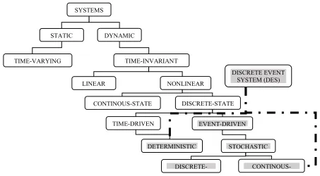
SYSTEMS

STATIC DYNAMIC

TIME-VARYING

NONLINEAR TIME-INVARIANT

Figure 1.2 Major Systems Classification (Cassanderas & Lafortune, 2010) DISCRETE-STATE LINEAR

EVENT-DRIVEN TIME-DRIVEN

CONTINOUS-STATE

DISCRETE-

CONTINOUS-DETERMINISTIC STOCHASTIC

(19)

4

2007). Different modelling methods are used for DEDS analysis such as Petri nets, generalized semi Markov processes, nonlinear programming, automata, computer simulation models and so on. It should be noted that the models used to describe DEDS are nonlinear in the conventional algebra. Recently, a class of DEDS called Max-Plus Linear has been defined (Seybold et al., 2015).

1.4.Discrete Event Systems Modeling Methods (Formal Methods)

DES has been applied to several fields of science and engineering. These fields of research apply different terminologies for DES methods. For example, in the field of industrial engineering, they are known as modelling methods. However, these methods are known as mathematical tools and formal methods in the fields of mathematics and computer science, respectively. Campos et al. (2014) define formal methods as mathematical techniques, often supported by tools, for developing “man-made systems”. These methods include Petri nets, Automata and Max-Plus Algebra. In another study, Li and Al-Ahmari (2013) call formal methods major mathematical tools for system development. They classify Automata, State Charts, Petri nets, Graph Theory, Process Algebra, Queueing Networks, and Temporal Logic as formal methods.

Although these methods are known as modelling methods in the fields of electrical, automation and control engineering, there are some other differences in the subdivision of terminologies. For instance, node definition in the control field is similar to merging point, and the rout is the sequence of series stations in the field of industrial engineering. Cassanderas and Lafortune (2010), Heidergott et al. (2006), and Baccelli et al. (1992) provide more information. Some of the most important and famous modelling methods in DES are considered below.

1.4.1. Petri Nets

Petri nets models were developed by C.A Petri in the early 1960s. Petri Net is a weighted bipartite

graph (𝑃, 𝑇, 𝐴, 𝑤) where 𝑃, 𝑇, 𝐴 and 𝑤 are a set of places, transitions, arcs, and weighted functions

on the arcs respectively. Transitions represent events that may occur, places are the input of the transitions, and finally, arcs define which places are preconditions or post conditions for each transaction. Arcs never connect two places or transactions together. Input and output places of a transition are places from which and to which an arc runs to a transition. Places might possess a discrete number of marks called token, which are fired by transitions as an input and turn to tokens

in output places (Cassandras & Lafortune, 2010).

(20)

5

𝑃 = {𝑝 , 𝑝 , 𝑝 } 𝑇 = {𝑡 , 𝑡 , 𝑡 }

𝐴 = {(𝑝 , 𝑡 ), (𝑝 , 𝑡 ), (𝑝 , 𝑡 ), (𝑝 , 𝑡 )}

𝑤(𝑝 , 𝑡 ) = 1, 𝑤(𝑝 , 𝑡 ) = 1, 𝑤(𝑝 , 𝑡 ) = 1, 𝑤(𝑡 , 𝑝 ) = 1, 𝑤(𝑡 , 𝑝 ) = 1, 𝑤(𝑡 , 𝑝 ) = 1,

𝑤(𝑝 , 𝑡 ) = 1, 𝑤(𝑡 , 𝑃 ) = 1,

The two main drawbacks of modelling DEDS with Petri Nets are: 1) graphic representation of complex systems is quite intricate, and 2) Indicating priorities and order is important; however, it is hard to manage when the system is complex.

1.4.2. Automata

DES is comprised of a set of states (𝑋) and events (𝐸) that cause transactions of these states. The

event sequences describe the behaviour of a system and the order in which the events arise. However, the time of events' occurrence is unspecified, which associates it to an untimed and

logical level of DES abstraction. This kind of DES is modelled by a language. If an even 𝐸 is

assumed as the alphabet, the sequence of events can configure strings (words). Finally, a language

is a set of those strings (Cassandras & Lafortune, 2010).

Automata is a tool that represents a language based on the comprehensible rules. It is comprised of

an even set 𝐸, 𝑋, transition functions, inthe initial state 𝑋 and marked state 𝑋 .

𝑡

𝑝

𝑝 𝑝

𝑡

Figure 1.3 Simple Petri Net Model

Figure 1.4 Simple Example of Automata Model 𝑗

𝑘 _{𝑖, 𝑘}

x

y

z

(21)

6

Assume 𝐸 = {𝑖, 𝑗, 𝑘}, then the transaction function of 𝑓: 𝑋 × 𝐸 → 𝑋 is represented graphically by

arcs:

𝑓(𝑥, 𝑗) = 𝑥, 𝑓(𝑥, 𝑘) = 𝑦, 𝑓(𝑧, 𝑗) = 𝑥 , 𝑓(𝑧, 𝑖) = 𝑖, 𝑓(𝑦, 𝑖) = 𝑓(𝑧, 𝑘) = 𝑧

The notation 𝑓(𝑥, 𝑘) = 𝑦 means that if the automaton is in state 𝑥, then upon of event 𝑘 occurrence,

the automaton will make a transition to state 𝑦 .

The main drawback of this way of modelling DES is space explosion, which occurs when a large number of automata are composed. A detailed description of automata can be found in Cassandras and Lafortune (2010) chapter two.

1.4.3. Markov Process

Suppose a sequence of possible events 𝑥 , 𝑥 , 𝑥 , … , 𝑥 observed at times 𝑡 , 𝑡 , 𝑡 , … , 𝑡 . Let 𝑥

be the present state of the process at 𝑡 and past history as {𝑥 , 𝑥 , 𝑥 , … , 𝑥 }; then the future

states {𝑥 , 𝑥 , 𝑥 , … } is completely independent of the past. Each event relies on the

previous event. This is referred to as the memoryless property of the Markove Process. Markov Chain is a stochastic model of the Markove Process in which the future is conditionally independent of past events. In other words, the past and present information is summarized in the present state to probabilistically attain the future. There are two types of Markove Chains called Discrete-Time and Continuous-Time. In the Discrete-Time Markove Chain, the events happen at time instances; however, in Continuous-Time the state transitions occur at time intervals.

1.4.4. Queuing Model

(22)

7 1.4.5. Discrete Events Simulation

Simulation is an imitation of a real-world process/system over time by generating the history of a system. The system behaviour is studied by developing a simulation model. In some cases, the developed model can be solved using mathematical methods, differential calculus, algebraic methods etc. However, in reality, some systems are too complex to yield analytical methods. In these cases, simulation can be used to emulate the behaviour of the system over the time.

1.5.Max- Plus Algebra

Max-Plus Algebra is a new mathematical tool that has been developed in theoretical and practical subjects. For example, Max-Plus has been used in theories such as Set theories, Graph theories, Queuing theories and Computational theories. More details about Max-Plus Algebra can be found in Chapter 2. The relevant literature is expressed in three groups as follows.

Since 1996, De Schutter and his research group they have published 46 articles and books in the field of Max-Plus Algebra and discrete event system such as linear systems modeling (2014), computational techniques (2015), approximation approaches (2011), Model Predictive Control (2001), and practical studies in traffic, transportation, automation and control systems issues (2016).

Gaubert. S (1997) has classified tropical semirings and the family of Max-Plus. He introduced basic techniques to solve Max-Plus linear equation. This is followed by studies in the field of graph theory as well as language theory. Later, Marianne et al. (2001) have declared Convex map that is monotone (preserve the product ordering) and no expansive. They presented the fixed point set when it is nonempty is isomorphic and its dimension strongly connected to components of a critical graph.

Cohen et al. (1998) have summarized the theoretical aspects of Max-Plus achievements through examples. The state space equations, canonical equations, transfer functions, asymptotic behaviour and eigenvalues, stabilization and resource optimization, geometric theories, etc. were discussed as some part of Max-Plus dependent contents.

(23)

8

in section 2.3. Consequently, a High-Speed algorithm is suggested by Goto and Ichige, (2010) to speed up the effect of calculating the Kleene Star for a weighted adjacency matrix. Moreover, they have studied applications of Max-Plus Algebra in other fields such as integer programming (2017), feedback control approach (2010), output constraints (2009), and linear systems (2007).

Adzkiya et al. (2016) have studied Max-Plus Linear (MLP) systems calculation tools. The proposed procedure is based on partitioning the state space and dynamics into regions. The results present finite-state transition systems that either simulate or bi-simulate the original MPL system. Bi-simulation equivalence aims to identify transition systems with the same branching structure, and which thus can simulate each other in a stepwise manner (Baier and Katoen, 2008).

Two optimization problems in Max-Plus Algebra related to the minimization of a product of triangular matrices have been defined by Bouquard et al. (2006). The first problem is a polynomial time optimization algorithm for scheduling a single or two-machine flow shop problem in 2×2 matrices products. The second problem considers the 3×3 matrices, which are shown as NP-hard. They have used a branch-and-bound algorithm to solve it.

Hardouin et al. (2017) have designed an observer-based controller for Max-Plus Linear systems solved in two steps: first, an observer computes the state estimation by using input and output measurements; afterwards these estimates are used to compute the state-feedback control system. This method provides better control than output feedback control, which was common.

Leela-Apiradee et al. (2017) have introduced a closed form of the L-localized solution set of Max-Plus interval linear system and its application to the optimization problem. The feasible set of an optimization problem has been simplified by the number of union set reduction.

Imaev and Judd (2008, 2009) have simplified and reduced the Max-Plus equations. The network connection of blocks was transferred to compose one block that has the same input and output structure. This means, a block defined as a combination of several stations instead of one station. In a block diagram the interconnection of a station with other stations were specified using routing matrices. Furthermore, a new topological method for evaluating the results of the synchronous matrix have been examined (2010). Properties of signal flow graphs (SFGs) over Max-Plus Algebra

are investigated, which are referred to as synchronous. Finally, a theory of synchronous a matrix

signal flow graph (MSFG), as a pictorial presentation of a set of linear matrix equations, has been

addressed in their studies.After proving the hypothesis, a single machine or a factory was used as

(24)

9

Adzkiya et al. (2016) have developed a software tool called VeriSIMPL2 for Max-Plus Linear (MPL) systems. The proposed procedure is based on partitioning the state space and dynamics into partitioning regions. This open-source software generates finite abstractions of autonomous MPL systems and enables formalization of general properties to be logical. The results present finite-state transition systems that either simulate or bisimulate the original MPL system.

Dealing with stochastic systems have enforced researchers to define uncertain conditions. Using statistical distribution likewise Poisson or Binomial are common in queueing network. Kaise and McEneaney (2015) have applied idempotent methods included Max-Plus basis-expansion approaches as well as curse-of-dimensionality-free methods to stochastic control and games. Curse of dimensionality refers to nonlinear modelling because in this modelling the computational cost and space dimension expanded exponentially. To conquer uncertainty using intervals instead of deterministic variables is extended among Max-Plus studies. In one of the latest studies, Wang and Tao (2016) have proved existence and uniqueness of a strong solution through a polynomial algorithm for such Max-Plus Linear equations. Other than that, Imaev and Judd (2010), Leela-Apiradee et al. (2017), Seybold et al. (2015) and Majdzik et al. (2016) have worked in the domain of stochastic system using Max-Plus. Table 1-1 provides a summary of Max-Plus Algebra theories and relevant research.

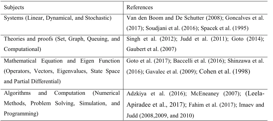
Table 1-1 Max-Plus Algebra developed theories

References Subjects

Van den Boom and De Schutter (2008); Goncalves et al. (2017); Soudjani et al. (2016); Spacek et al. (1995) Systems (Linear, Dynamical, and Stochastic)

Singh et al. (2012); Judd et al. (2011); Goto (2014); Gaubert et al. (2007)

Theories and proofs (Set, Graph, Queuing, and Computational)

Goto et al. (2017); Baccelli et al. (2016); Shinzawa et al. (2016); Gavalec et al. (2009); Cohen et al. (1998) Mathematical Equation and Eigen Function

(Operators, Vectors, Eigenvalues, State Space and Partial Differential)

Adzkiya et al. (2016); McEneaney (2007);

(Leela-Apiradee et al., 2017); Fahim et al. (2017); Imaev and

Judd (2008,2009, and 2010) Algorithms and Computation (Numerical

Methods, Problem Solving, Simulation, and Programming)

In this part, the application of Max-Plus Algebra in the manufacturing system is discussed.

(25)

10

composed sequences to be executed by the various machines are fixed. They proved that computational tools coming from Max-Plus Algebra provide an effective way to write the performance indexes in terms of the decision variables representing the binary alternatives.

In addition to developing mathematical theories, Imaev and Judd (2008 & 2009) have developed several modelling approaches in manufacturing systems using Max-Plus Algebra. At first they proposed hierarchical modelling for any deterministic manufacturing system. Then Block Diagram-Based modelling is suggested. A manufacturing system constitutes a network of processing elements. A block with two inputs and two outputs expresses one of the processing elements. A block is defined as a single manufacturing operation, a single machine, a single part, or a factory. Combination of two or more blocks which have same input/output structure, can be seen as a hierarchical model. In such way a huge and complex manufacturing system can be broken into smaller ones (sub-system).

Beyond these studies Imaev and Judd (2010) have defined a block as a 3×3 matrix. Moreover, a class of signal flow graphs (SFGs) was introduced called matrix signal flow graphs (MSFGs). They have called a SFG over Max-Plus Algebra a synchronous SFG, because maximization operation represents synchronization phenomena in discrete event systems. Three topological methods: 1) basic graph reduction rules, 2) return loop method, and 3) basic manufacturing blocks; are applied to evaluate the results of synchronous. Also, machine-based and part-based modelling approaches have been introduced and compared. The part-based approach is preferred for scheduling application; however, machine-based is suggested for buffer allocation. Both approaches give the same result for makespan.

(26)

11

and then using these equations, data analysis only took a few seconds. However, generating and executing discrete event simulation models requires many runs and takes days.

In another study, Seleim and ElMaraghy (2014b) have modelled Mixed-Model Assembly Lines (MMALs) with both closed and open stations by using Max-Plus Algebra. For verification, two numerical examples have been presented. In the first example, an assembly line containing four stations with three different outputs were considered. Three possible product mix variants sequences have been compared and the optimal point for each sequence was founded. The second example studied the effect of changing launching rate of work units of line performance. Their parametric analysis as a method has provided a better understanding for designers. It allows designers to analyze stations sensitivity to the changes in assembly line and their effects on idle time and line length. In addition, decision makers can use the presented analyses to assess whether the improvements can affect the current sequence optimality and if it is needed to increase line capacity by changing launching rate.

Seybold et al. (2015) have introduced a predictive control framework to fault-tolerant control and used Max-Plus Algebra to model battery assembly system. This system is included five stations and two input. The robustness issues which are inevitable in real production systems have been discussed. They show an illustrative example which clearly exhibits the high performance of the proposed approach while all productivity demands are incorporated within the constraints.

Afterward, Majdzik et al. (2016) have represented a framework for fault-tolerant of a battery assembly line (9 stations and considering transportation time). The proposed approach is based on an interval analysis approach, which along with Max-Plus Algebra allows describing uncertain discrete event system such as production line. As a result, the performance of the pilot implementation has validated the recommended strategy for advanced battery assembly system. The recommended approach examined single as well as simultaneous fault concerning processing, transportation and mobile robots.

The proposed solution by Leela-Apiradee et al. (2017) has been applied in product pricing problem that is composed of, 6 parameters (3 products and 3 customers) and 9 constraints. By considering customer purchasing power and cost of transportation an acceptable solution is presented.

(27)

12

analytical approach. A system composed of 6 stations with Poisson arrival and bottleneck placed at the fifth station was considered. To minimize the capacity of the buffer, various models were designed by changing the placement of the bottleneck and the sequence of processing times. They expressed, the actual sojourn times are affected by the buffer capacities and processing time sequence. Table 1-2 illustrates some of the latest research on Max-Plus Algebra.

Table 1-2 Max-Plus Algebra Application

References Application Group

Imaev and Judd (2007,2008,2009); Seleim and ElMaraghy (2014a,2014b); Majdzik et al. (2017)

Modelling (Mathematical and Systems )

Bouquard et al. (2005); Seybold et al. (2015); Adzkiya et al. (2016); Hochang et al. (2016); Kersbergen et al. (2016); Han et al. (2017); Leela-Apiradee et al. (2017)

Performance and System Optimization, evaluation and Simulation

Febbraro et al. (1994); Yun-Xiang et al. (2016); Singh et al. (2012 & 2013)

Scheduling, Planning (Real-Time Systems) and Computer Simulation

Hardouin et al. (2017); Song et al. (1998); Dias et al. (2015, 2016)

Control (Theory, Systems, Feedback, Predictive Robotics and Automation)

Modelling DES can be classified based on industrial applications. Particularly, a number of articles focused on the industrial applications of Max-Plus Algebra have been mentioned below.

A predictive controller model, as well as railway traffic for online traffic management of railway networks with a periodic timetable, have been considered by Kersbergen et al. (2016). The railway system is described by a switching Max-Plus Linear Model. The measurement of running, dwell times and future running times are assumed to be available. The switching Max-Plus linear model for the railway is used to determine optimal dispatching actions, by recasting that problem as a Mixed Integer Linear Programming (MILP) problem.

Heidergott et al. (2006) have applied the foregoing technique for Dutch passenger train network. Consequently, Case (2010) has modelled a simple railway network as a part of the Dutch train transportation system. Two transit stations supposed to have interconnection plus their connection with outside. This model is involved at least for 440 trains.

Han et al. (2016) have applied a Max-Plus Algebra model to develop a general framework for

(28)

13

as fuel consumption and flight delay. The constraints between input and output variables based on the observation that jet route can be divided into different sub-segments were obtained. The performance of system resources proposed by Max-Plus has been verified through simulations. Table 1-3 represents some of the related researches in different industries.

Table 1-3 Max-Plus Algebra industries usages

Industrial Applications References

Automation and Control Van den Boom et al. (2000-2018); Addad et al. (2008-2012); Armstrong et al. (2014), Ahmane et al. (2006); Goto et al. (2010)

Transportation Kersbergen et al. (2008); Van den boom et al. (2000-2016); Han et al. (2017, 2016); Haddad et al. (2016); Shang et al. (2010); Case J (2010)

Manufacturing Febbraro et al. (1994); Seleim and ElMaraghy (2014 a, 2014b); Majdzik et al. (2017); Hochang et al. (2016); Imaev et al. (2007,2008,2009); Gorji et al. (2013)

1.6.Advantages and Drawbacks of Max-Plus Algebra

A tool like Max-Plus Algebra certainly has some advantages and drawbacks; these are discussed below.

Advantages:

 The event timing dynamics of any deterministic system can be expressed by a set of linear

equation (Imaev & Judd, 2009; Muijsenberg, 2015; Seleim, 2016).

 Provides computational engine to calculate system's quantitative characteristics (Imaev &

Judd, 2009).

 Provides a strong framework for both modelling and analysis (Cassandras & Lafortune,

2010).

 The set of possible solutions can be obtained directly under a set of initial conditions

(Adzkiya et al., 2016; Imaev & Judd 2009).

 Can study the periodicity of a system in order to characterize the system behaviour

(Cassandras & Lafortune, 2010).

 Can be used in the analysis and control of manufacturing systems (Seleim, 2016).

 Can describe the order of the system's events (Wetjens, 2004).

 Researchers have benefited from the guidelines and concepts provided by Max-Plus

(29)

14

 Max-Plus is an appropriate method to model a system for short-term and small-sized

systems (Di Febbraro et al., 1994).

Drawbacks:

 The model should be defined for a certain level of complexity (Wetjens, 2004).

 Simultaneously, a model designer should deal with several difficulties such as

manufacturing structure and entities as well as mathematical formulation and calculate solution by Max-Plus operations over matrices (Seleim, 2016).

 The model structure is not flexible, whereby any changes in the system's structure will be

required to develop from the bottom (Muijsenberg, 2015). sometimes minor changes lead to an increase in the number of equations and dimensions of matrices (Seleim, 2016).

 The number of studies involved in this new area of the system theory for DES has remained

small compared with other tools (Cohen, 1997).

 There is not any available tool or software to facilitate modelling and analysis process

(Seleim, 2016).

 The type of models in the Max-Plus framework is limited to marked graphs and extensions

to stochastic DES are not easy (Cassandras & Lafortune, 2010).

 Performance evaluation is not executed in the field of comparison of Max-Plus with other

modelling methods, particularly for large instances (Houssin, 2011).

 Some fundamental shortages slow down the progress of the model (Cohen, 1997).

The weakness of DES modelling methods:

 Generally, DES modelling methods lead to nonlinear models.

 Discrete event simulation is usually computationally expensive and does not supply

equations needed to analyze and predict systems behaviour (Imaev & Judd 2008). Also, it is time-consuming and can give information only for the given simulated parameters of the system; numerous simulation runs would be required (Seleim, 2016).

 Queueing network and Markov chains are used to evaluate long-term performance

characteristics of systems, especially stochastic ones (Imaev & Judd 2008; Seleim, 2016).

 Timed-event graph and directed graphs are subclasses of Petri nets in which each place is

limited only to one incoming and one outgoing arc (Imaev & Judd, 2008).

 Simulation is certainly the most common tool for DESs and requires a high level of detail,

(30)

15 1.7.Research Gap Analysis

In this section the relevant literature is considered critically. Recently, Max-Plus Algebra has been expanded among scholars and academics. Since this high interest in the Max-Plus tool is limited to the last two decades, Max-Plus Algebra requires further justifications and verifications.

Since the 1980s, Max-Plus Algebra has broadly been developed in theories. However, few researchers have examined the application of Max-Plus in engineering fields, particularly in manufacturing systems (Leela-Apiradee et al., 2017). In spite of that, the use of Max-Plus Algebra in practical and real-life systems has not been expanded sufficiently. Cohen et al. (1998) declare that the application of Max-Plus did not receive enough attention. This phenomenon is clear by comparison of the number of publication in theories and applications.

Despite progress in Max-Plus theories, developed algorithms and proposed computational methods (Seleim, 2016; Imaev, 2009), there are still difficulties with its calculation steps. Max-Plus is constructed by matrices and numerous equations. Difficulties in calculation have limited users to those who have enough knowledge in mathematics (Bouquard et al., 2006). In addition, due to these complex calculation steps, Max-Plus Algebra is suggested and applied for small-size problems.

To tackle the difficulties of Max-Plus calculation steps, the mathematical software has been used. The majority of researchers have benefited from Matlab and Mathematica as general software. However, this requires sufficient knowledge of language programming. Thus, to solve one issue another issue is raised. Consequtively, Adzkiya et al. (2016) have introduced an open-source software for verification of Max-Plus Linear (MLP) systems.

It is clear that Max-Plus Algebra as a linear mathematical modelling tool has not been expanded to accommodate the stochastic systems (Seleim, 2016). Interval system is a prominent method applied in the majority of suggested stochastic systems. To solve these linear systems, different heuristic models have been developed. Hence, there is a lack of application of a linear mathematical tool such as Max-Plus Algebra in this type of systems.

(31)

16

Discrete Event Simulation is the most popular method to model DES. However, the comparison of this method with Max-Plus has hardly been discussed in previous research.

By looking into the application of Max-Plus Algebra in industries, it has been noticed that most of the studies have been done in the fields of transportation, control, and automation. However, it is believed that there have not been enough studies in the field of manufacturing systems.

There have been a few scholars who applied Max-Plus Algebra in flow-line discrete manufacturing systems (Majdzik et al., 2016; Seybold et al., 2015; Seleim, 2016). However, there are other types of manufacturing systems processes and configurations, such as repetitive, continuous, cellular manufacturing, and job shop, that need to be modelled and tested using this mathematical tool.

Behaviour of a manufacturing system are broad and require more studies such as bypassing, disturbance (breakdown and downtime), backtracking/reentrancy (close and open loops, reworks and reschedule), alternative process, sourcing/allocation policies, buffer (converge and diverge) transportation method, etc. (Seybold et al., 2015; Majdzik et al., 2016; Imaev, 2009).

Finally, Max-Plus Algebra has been applied in optimization (Bouquard et al., 2006; Xiaoping et al., 2013), simulation (Becker & Latovetsky, 2011), scheduling (Di Febbraro, 1994; Kubo & Nishinari, 2018), planning (Abbou et al., 2017), performance evaluation (Singh & Judd, 2012) reconfiguration (Zhu et al., 2004), etc.

This study is a unique application of Max-Plus Algebra in line balancing of a manufacturing system. In this research, Line balancing a manufacturing system is modelled using Max-Plus Algebra. To do that seven scenarios are designed to find out the best combination of adding parallel identical stations and bottleneck. To analyze the designed scenarios, some Key Performance Indicators are defined. Finally, FlexSim as simulation software is used to verify the outcome of the Max-Plus model.

1.8.Research Scope

(32)

17

Firstly, this research provided a general method of line balancing a manufacturing system that can be extended to other types of discrete manufacturing systems. This model will help the manufacturer and industries to find the best answer to balance their manufacturing lines without changing the configuration of their flow line.

Secondly, the developed line balancing included seven scenarios. The first scenario was a simple flow line. Next scenarios have been designed based on previous scenarios by identifying bottleneck and critical path. The scenarios became more complex by adding parallel stations to the bottleneck and adding a finite buffer to the stations that their downstream process is a bottleneck.

Thirdly, several manufacturing Key Performance Indexes (KPIs) have been defined, such as Product Completion Time (Average Delivery Rate by the system in seconds), Total Processing Lead Time, Station's Utilization Rate, Idle Time and Efficiency of the System. Financial Analysis is formulated to compare all scenarios by using a combination of total processing lead time, utilization rate and etc.; these are used to evaluate the different scenarios. These KPIs can be extended to other modelling purposes.

Finally, the scenarios were tested using discrete event simulation tool (Flexim). Same data, parameters, variables and conditions, etc. were applied when simulating the scenarios to make the comparison with results from Max-Plus valid. Both Flexim and Max-Plus Algebra have resulted in the same outcomes. However, Max Plus Algebra was quicker and easier to manage.

1.9.Research Contributions

Firstly, this study represents a practical approach to use Max-Plus Algebra and proves how this method is easy to understand for decision makers with a little background or basic knowledge of mathematics.

Secondly, this research is the first study of the application of Max-Plus Algebra in line balancing of a discrete manufacturing system. This method is applied to different structures/configurations of a manufacturing system such as Series, Merged, Paralleled, Buffered and Combined.

Thirdly, the problem size of the developed model is at least twice that of previous studies (seven stations). The last scenario composed of 12 stations, 4 parallel identical stations and two buffers.

(33)

18

Finally, discrete event simulation like FlexSim is used to verify and compare the results obtained by using Max-Plus Algebra.

1.10. Thesis statement

The thesis statement of this research could be formulated as follows:

Max-Plus Algebra could be a competitive and fast tool in the field of modelling manufacturing system and analyze its line balancing results.

The competitive term in this study refers to the being easy to use for model designer and easy to change the structure, size and complexity of a system. The fast term refers to the time consumed for modelling process of a system. This research considered the period of time from designing point to analyze the results of modelled system under equal conditions in comparison with discrete event simulation tool like FlexSim. The advantages of Max-Plus Algebra are demonstrated in the Car Headlight manufacturing system as a practical case study.

1.11. Research overview

(34)

19

CHAPTER TWO

BASICS OF MAX-PLUS ALGEBRA AND MATHEMATICAL CONCEPTS

2.1. Introduction

This chapter presents an introduction to Max-Plus Algebras and shows their application in manufacturing systems.

2.2. Max-Plus Algebras

A Max-Plus Algebra is the set ℝ = ℝ ∪ {−∞}, where ℝ is the set of real numbers, together with the binary operators ⊕ and ⊗, where 𝑥⨁𝑦 = 𝑚𝑎𝑥(𝑥, 𝑦) and 𝑥⨂𝑦 = 𝑥 + 𝑦. For convenience we use the symbols ℯ = 0 and 𝜀 = −∞.

The following properties are satisfied by Max-Plus Algebras.

1. Associativity. For all 𝑥, 𝑦, 𝑧 ∈ ℝ we have 𝑥 ⊕ (y ⊕ z) = (𝑥 ⊕ y) ⊕ z and 𝑥 ⊗ (y ⊗ z) = (𝑥 ⊗ y) ⊗ z.

2. Commutativity. For all 𝑥, 𝑦 ∈ ℝ we have 𝑥 ⊕ y = y ⊕ x and 𝑥 ⊗ y = y ⊗ x. 3. Distributivity of ⊗ over ⊕. For all 𝑥, 𝑦, 𝑧 ∈ ℝ we have

𝑥 ⊗ (y ⊕ z) = (𝑥 ⊗ y) ⊕ (x ⊗ z).

4. Idempotency of ⊕. For all 𝑥 ∈ ℝ we have 𝑥 ⊕ 𝑥 = 𝑥.

5. Zero element: For all 𝑥 ∈ ℝ we have 𝑥⨁ε = 𝑥. 6. Unit element: For all 𝑥 ∈ ℝ we have 𝑥⨂𝑒 = 𝑥.

7. Zero absorption for ⊗: For all 𝑥 ∈ ℝ we have 𝑥 ⊗ ε = ε ⊗ 𝑥 = 𝜀. In future chapters we will need to use exponentiation. We define

𝑥⨂ = 𝑥⨂𝑥⨂ … ⨂𝑥 = 𝑥 + 𝑥 + ⋯ + 𝑥 = 𝑛𝑥.

2.3. Max-Plus Algebra over Matrices

Let 𝐴, 𝐵, 𝐶 ∈ ℝ × _{and let [𝐴]} _{be the}_{𝑖, 𝑗th element, that is, the element in row}_ⅰ_and column 𝑗, of the matrix 𝐴. Thus, we have that, if 𝐶 = 𝐴⨁𝐵 then

(35)

20

The 𝑚 × 𝑛 zero matrix is denoted by ℰ × and is given by [ℰ × ] = 𝜀. Note that 𝐴⨁ℰ = 𝐴.

Now we define matrix multiplication. Let 𝐴 ∈ ℝ × and 𝐵 ∈ ℝ × . If 𝐶 = 𝐴⨂𝐵 then

[𝐶] = [𝐴⨂𝐵] = 𝑝 ⨁ 𝑙 = 1

[𝐴] ⨂[𝐵] .

The 𝑛 × 𝑛 identity matrix is denoted by 𝐸 and is given by [𝐸 ] = 𝑒, if 𝑖 = 𝑗, and

[𝐸 ] = 𝜀, otherwise. For any matrices 𝐴 ∈ ℝ × _{and 𝐵 ∈ ℝ} × _{we have that}

𝐴⨂𝐸 = 𝐴 and 𝐸 ⨂𝐵 = 𝐵.

For matrix exponentiation, we have 𝐴⨂ _{= 𝐸} _and 𝐴⨂ = 𝐴⨂𝐴⨂ … ⨂𝐴 .

The Kleene star operator on A ∈ ℝ × _{is denoted by 𝐴}∗_{and is given by}

𝐴∗= 𝐴⊗ ⊕ 𝐴⊗ ⊕ … ⊕ 𝐴⊗ = ∞ ⊕ 𝑛 = 0

𝐴⊗ .

Through the rest of the thesis, the ⊗ operator will be omitted whenever its use is obvious,

thus 𝑎 ⊗ 𝑏 ⊕ 𝑐 ⊗ 𝑑 will be written as 𝑎𝑏 ⊕ 𝑐𝑑 or 𝐴⊗ _{as 𝐴} _.

A set of linear equations in a Max-Plus Algebra, see, for example, Heidergott et al. (2006) and Baccelli et al. (2001), can be written as

𝑋 = 𝐴𝑋 ⊕ 𝐵𝑈 (2.1)

which has the solution

𝑋 = 𝐴∗_𝐵𝑈.

2.4. Modelling A Manufacturing System Using Max-Plus Algebra

Using a development is similar to

(36)

21

Let the processing times for stations 1, 2, 3 and 4 be 𝑡 , 𝑡 , 𝑡 , and 𝑡 , respectively. The time instants that raw material for part 𝑘 is fed to the stations 1 and 2 are 𝑢 (𝑘) and 𝑢 (𝑘) respectively. The starting time of operation for processing part 𝑘 in stations 1, 2, 3 and 4 are denoted by 𝑥 (𝑘), 𝑥 (𝑘), 𝑥 (𝑘) and 𝑥 (𝑘), respectively. The time instants of the finished part 𝑘 at the last station is 𝑦(𝑘).

The equations for each stations 1 and 2 are

𝑥 (𝑘) = 𝑢 (𝑘)⨁𝑥 (𝑘 − 1)𝑡 , and (2.2)

𝑥 (𝑘) = 𝑢 (𝑘)⨁𝑥 (𝑘 − 1)𝑡 . (2.3)

Since station 3 is in series after station 1 we have

𝑥 (𝑘) = 𝑥 (𝑘)𝑡 ⨁𝑥 (𝑘 − 1)𝑡 . (2.4)

Combining (2.2) and (2.4) we have

𝑥 (𝑘) = 𝑢 (𝑘)𝑡 ⨁𝑥 (𝑘 − 1)𝑡 ⨁𝑥 (𝑘 − 1)𝑡 . (2.5) Since the station 4 is a merging point we use (2.3) and (2.5) to get

𝑥 (𝑘) = 𝑥 (𝑘)𝑡 ⨁𝑥 (𝑘)𝑡 ⨁𝑥 (𝑘 − 1)𝑡 . (2.6) By substituting (2.3) and (2.5) into (2.6) we get

𝑥 (𝑘) = 𝑢 (𝑘)𝑡 𝑡 ⨁𝑥 (𝑘 − 1)𝑡 𝑡 ⨁𝑥 (𝑘 − 1)𝑡 ⨁𝑢 (𝑘) 𝑡 ⨁𝑥 (𝑘 − 1)𝑡 ⨁𝑥 (𝑘 − 1)𝑡 . (2.7) Since the arrival time of the finished product 𝑘 is equal to the starting time of processing at station 4 plus processing time of station 4 we get

𝑌 = 𝑥 (𝑘)𝑡 . (2.8)

We combine equations (2.2),(2.4), (2.5) and(2.7) to get

𝑋 = 𝐴𝑋 ⨁𝐵𝑋 ⨁𝐷𝑈 (2.9)

and we can rewrite (2.8) to get

𝑌 = 𝐶𝑋 , (2.10)

where

𝑋 = 𝑥 𝑥 𝑥 𝑥

, 𝑈 = 𝑢_𝑢 ,

Figure 2.1 A mixed manufacturing system Station1

U1

U2

Station 3 Station 2

(37)

22 𝐴 = 𝜀 𝜀 𝜀 𝜀 𝜀 𝜀 𝜀 𝜀 𝑡 𝜀 𝜀 𝑡 𝜀 𝑡 𝜀 𝜀 , B= 𝑡 𝜀 𝜀 𝜀 𝜀 𝑡 𝜀 𝜀 𝜀 𝜀 𝜀 𝜀 𝑡 𝜀 𝜀 𝑡 , 𝐷 = 𝑒 𝜀 𝜀 𝜀 𝜀 𝑒 𝜀 𝜀 and 𝐶 = [𝜀 𝜀 𝜀 𝑡 ]. Since 𝐴 = ℰ for 𝑛 > 3,

𝐴∗= 𝑒 𝜀 𝜀 𝜀 𝜀 𝑒 𝜀 𝜀 𝜀 𝜀 𝜀 𝜀 𝑒 𝜀 𝜀 𝑒 ⨁ 𝜀 𝜀 𝜀 𝜀 𝜀 𝜀 𝜀 𝜀 𝑡 𝜀 𝜀 𝑡 𝜀 𝑡 𝜀 𝜀 ⨁ 𝜀 𝜀 𝜀 𝜀 𝜀 𝜀 𝜀 𝜀 𝜀 𝑡 𝑡 𝜀 𝜀 𝜀 𝜀 𝜀 𝜀 = 𝑒 𝜀 𝜀 𝜀 𝜀 𝑒 𝜀 𝜀 𝑡 𝑡 𝑡 𝜀 𝑡 𝑒 𝑡 𝜀 𝑒 . We define 𝐴 = 𝐴∗𝐵 = 𝑒 𝜀 𝜀 𝜀 𝜀 𝑒 𝜀 𝜀 𝑡 𝑡 𝑡 𝜀 𝑡 𝑒 𝑡 𝜀 𝑒 𝑡 𝜀 𝜀 𝜀 𝜀 𝑡 𝜀 𝜀 𝜀 𝜀 𝜀 𝜀 𝑡 𝜀 𝜀 𝑡 = 𝑡 𝜀 𝜀 𝜀 𝜀 𝑡 𝜀 𝜀 𝑡 𝑡 𝑡 𝜀 𝑡 𝑡 𝑡 𝜀 𝑡 and 𝐵 = 𝐴∗𝐷 = 𝜀 𝜀 𝜀 𝜀 𝜀 𝜀 𝜀 𝜀 𝑡 𝑡 𝑡 𝜀 𝑡 𝜀 𝑡 𝜀 𝜀 𝑒 𝜀 𝜀 𝜀 𝜀 𝑒 𝜀 𝜀 = 𝑒 𝜀 𝜀 𝑡 𝑡 𝑡 𝑒 𝜀 𝑡 .

According to Seleim (2016), equation (2.9) can be rewritten as:

𝑋 = 𝐴𝑋 ⨁𝐵𝑈 (2.11)

where 𝐴 = 𝐴∗_{𝐵 and 𝐵 = 𝐴}∗_𝐷.

For example, if we set 𝑡 = 2, 𝑡 = 3, 𝑡 = 4, and 𝑡 = 1 we get

𝐴∗ ₌ 𝑒 𝜀 𝜀 𝜀 𝜀 𝑒 𝜀 𝜀 2 6 𝜀 3 𝑒 4 𝜀 𝑒 , 𝐴 =

2 𝜀 𝜀 𝜀

𝜀 3 𝜀 𝜀

2 6 𝜀 3 4 4 𝜀 1

, and 𝐵 =

𝑒 𝜀 𝜀 2 6 𝑒 𝜀 3

giving the main equation of the system

𝑋 =

2 𝜀 𝜀 𝜀

𝜀 3 𝜀 𝜀

2 6 𝜀 3 4 4 𝜀 1 𝑥 𝑥 𝑥 𝑥 ⊕ 𝑒 𝜀 𝜀 2 6 𝑒 𝜀 3 𝑢 𝑢 . 2.5. Summary

(38)

23

CHAPTER THREE

MODELLING OF MANUFACTURING SYSTEM BY MAX-PLUS ALGEBRA

3.1.Introduction

In chapter two, the basic context of Max-Plus Algebra were discussed. In this chapter, variables, state space description, assumptions, and modelling the different structure of a manufacturing system using Max-Plus Algebra are explained.

3.2.General Proposition of a Model using Max-Plus Algebra

3.2.1. Variables

To model a manufacturing system, the definition of entities needs to be clear. Inputs, variables and output of the station i as a member of the manufacturing system are modelled and assumed as below:

K: an event counter, which is the number of parts (jobs),

𝑡: denotes processing time of station i,

𝑈 (𝑘): denotes the time instants at which incoming part k is fed to the station i,

𝑥 (𝑘): denotes the time instants when station i starts processing part k,

𝑦(𝑘): stands for the time instants at which part k is completed and leaves the line as a finished product.

3.2.2. State Space Description

In the systems theory, the term state has a precise meaning and it describes behaviour of a system at a time instant in a measurable way. The state space of a system is the set of all possible values

Figure 3.1 A simple structure of a system

X(k) t

M _Y(k)

(39)

24

(usually denoted by 𝑋) (Cassandras & Lafortune, 2010). In this study, corresponding state variables such as U(k), X(k), Y(k), rely on part 𝑘 which makes the system dynamic by considering events of such system that evolve in time. Two primary conditions are assumed in this system. First, the input (U), such as raw material or part, is available with no arrival time. Second, each station starts processing part 𝑘 + 1 when part 𝑘 leaves the station. As discussed in chapter two, the state equations are represented in several different forms. However, the common form is based on differential equations as below:

𝑋(𝑘 + 1) = max (𝑈(𝑘 + 1), 𝑋 (𝑘) + 𝑡 ) or

𝑋(𝑘 + 1) = 𝑚𝑎𝑥(𝑋 (𝑘 + 1) + 𝑡 , 𝑋 (𝑘) + 𝑡 )

3.2.3. Assumptions in the Manufacturing System

The following assumptions are considered in the developed general model; otherwise, it will be noted.

1- Process time of stations is deterministic and fixed.

2- All stations have infinite buffers.

3- First In, First Out (FIFO) operation rule is followed.

4- The process sequence is based on production flow line.

5- The station only processes one part at a time.

6- Stations do not have any failure, downtime or stoppage.

7- The process time includes loading time, operation time, and unloading time.

3.3.Modelling of a Manufacturing System

(40)

25 3.3.1. Modelling "n" Series Stations

In this structure, stations are laid out consecutively. There is no merged point, parallel station or buffer. Parts are processed by passing through all stations. This structure is shown in Fig. 3.2 can be explained by Max-Plus equations as follows:

By following the main equation (2.8) the main state equation is:

𝑋(𝑘) = 𝐴𝑋(𝑘 − 1) ⊕ 𝐵𝑈(𝑘) (3.1)

where:

𝐴 = 𝐴∗⊗ 𝐵 = ⎣ ⎢ ⎢

⎡ 𝑡 𝜀 … 𝜀

𝑡 𝑡 𝜀

⋮ ⋮ ⋱ ⋮

𝑡 𝑡 . . 𝑡 𝑡 𝑡 . . 𝑡 … 𝑡 𝑡 ⎦ ⎥ ⎥ ⎤

and B = A∗_{⊗ D =}

e t

⋮ t t . . t

From the main equation it can be deduced that for any station i, the state equation for the part k is equal to:

X, = t X, ⊕ t X , ⊕ t t X , ⊕ … ⊕ t t … t X , ⊕ t t … t U

Therefore, the Max-Plus equation can be generated directly by state equation (3.1) with any number of stations.

3.3.2. Modelling "n" Merged Stations

The merged station is a station that receives input from more than one station. Hence, state of part

k at station ⅰ is calculated by considering the main state equation as (3.1), where A and B will be: 𝑡

X₁ X_i

U 𝑡 𝑡

X_n

Y

(41)

26 𝐴 = 𝐴∗_{⊗ 𝐵 =}

⎣ ⎢ ⎢ ⎢ ⎢

⎡𝑡 𝜀 … 𝜀

𝜀 𝑡 𝜀

⋮ ⋱ ⋮

𝜀 𝜀 𝑡 𝜀

𝑡 𝑡 … 𝑡 𝑡 ⎦⎥ ⎥ ⎥ ⎥ ⎤

, and 𝐵 = 𝐴∗_{⊗ 𝐷 =}

⎣ ⎢ ⎢ ⎢

⎡ 𝑒_𝜀 𝜀_𝑒 … 𝜀_𝜀

⋮ ⋱ ⋮

𝜀 𝜀 𝑒 𝜀

𝑡 𝑡 … 𝑡 ⎦

⎥ ⎥ ⎥ ⎤

3.3.3. Modelling Parallel Identical Stations

In section 3.3.1, modelling n series stations, it has been assumed that there is no parallel station in the system. However, adding a parallel station is one of the ways to reduce idle time, which is a priority for manufacturers. In other words, the bottleneck station gets one or more identical stations, which lead to tasks distribution among those parallel stations. For example, if an identical station is added to station i, while this station is processing part k, the identical station processes the next part (k+1).

As shown in figure (3.4), m parallel stations are added to station i. These stations can be assumed to be one station for the purpose of modelling. Therefore, the condition that the station should have finished processing part 𝑘 − 1, would be replaced by 𝑘 − 𝑚. The conditions for the first and last stations are unchanged. Thus, all variables are similar to the series model, except matrix B, which would be represented by two matrices. The first matrix is the same as matrix B, but the difference is that all entities in the corresponding column of the parallel station are replaced with 𝜀.

Likewise, 𝐵 =

𝑡 𝜀 𝜀

𝜀 𝜀 𝜀

𝜀 . . ⁞. . 𝑡

and 𝐵 =

𝜀 𝜀 𝜀 𝜀 𝑡 𝜀 𝜀 𝜀 𝜀

The main equation will have an extra nominal for each group of parallel stations and evolves to: Y

𝑡 𝑡 𝑡

U₁₁ U_1i U_1n

𝑡

𝑡 𝑡

X₁ Xi

U

X_n

Y 𝑡

𝑡

Figure 3.4 Flow line with the parallel identical station Figure 3.3 "n" merged stations

(42)

27

𝑿 = 𝑨𝑿 ⊕ 𝑨𝑷𝒊𝑿 ⊕ 𝑩𝑈 (3.2)

3.3.4. Modelling A Station with Finite Buffer

Buffering is one of the ways that manufacturers are using to account for fluctuations and variations in their systems. Buffers can be raw material storage, finished part inventories, and unfinished parts. Assuming the station has a buffer with B parts changes the main state equation as below:

𝑿 = 𝑨𝑿 ⊕ 𝑩𝑈 ⊕ 𝑨𝑩𝒊𝑿 (3.3)

In which matrices 𝐴, and 𝐵 are same as before and 𝐴𝐵 is added as below:

𝑨𝑩𝒊=

⎣ ⎢ ⎢ ⎢ ⎢ ⎢

⎡𝜀_⋮ … 𝜀_⋮ 𝜀_⋮ … 𝜀_⋮ 𝜀

𝜀 … 𝜀 𝑒 𝜀

⋮ ⋮ 𝜀 ⋮ ⋮

⋮

𝜀 … 𝜀 𝜀 𝜀 𝜀 ⎦ ⎥ ⎥ ⎥ ⎥ ⎥ ⎤

3.3.5. An Integrated Model (Series, Merged, Parallel Stations and Finite Buffer)

The last structure is the combination of all the previous station models. In the real world, a manufacturing system takes advantage of using both parallel station(s) and buffer(s) to balance the production line. By using the parallel station at a bottleneck and buffers at stations whose upstream process is the bottleneck, the production flow would be smoother. By having all systems structures such as series, merged, parallel station and finite buffer in one system, the main equation is changed as below:

𝑿 = 𝑨𝑿 ⊕ 𝑩𝑈 ⊕ 𝑨𝑷𝒊𝑿 ⊕ 𝑨𝑩𝒊𝑿 (3.4)

The matrices’ structure should be similar to those matrices that were discussed in previous models. 𝑡

𝐁𝐮𝐟𝐟𝐞𝐫

X₁ Xi

U

X_n

Y

𝑡 𝑡

(43)

28

3.4.The General form of Modelling Formulation using Max-Plus Algebra

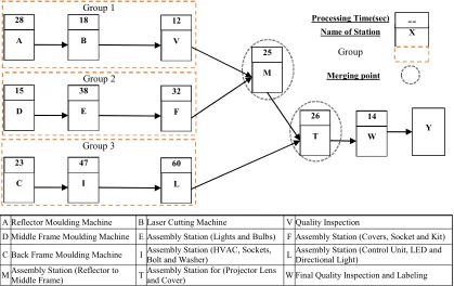
In this research, a general form of the manufacturing system is composed of three parallel stages each of which has three stations in series, two merged stations, and a series of finishing stations. Figure 3.7 represents the overall view of the considered manufacturing system. To make it easy to understand, the general framework does not include any parallel stations or buffers. In this section, the Max-Plus Algebra equations related to this framework are explained, and more details will be discussed in chapter 4.

Using Max-Plus Algebra, the system's framework and behaviour can be modelled by the next state equations. Variables, state space and assumptions are the same as the general form explained in section (3.2).

The following equations are applied for each station:

Group 1, stations A, B and, V:

Station A: 𝑥 (𝑘) = 𝑢 (𝑘)⨁𝑥 (𝑘 − 1)𝑡 (3.5) m

𝑡

X₁ X i

U

X _n

Y

1 _𝑡

Figure 3.6 An integrated model (Series, Merged, Parallel Stations and, Finite Buffer)

𝑡

𝐁𝐮𝐟𝐟𝐞𝐫