Essays on Multivariate Stochastic Volatility Models Using Wishart Processes: A General Discussion and Dimension Reduction by Latent Factor Structures.

(1)

Abstract

KU, YU-CHENG. Essays on Multivariate Stochastic Volatility Models Using Wishart Processes:

A General Discussion and Dimension Reduction by Latent Factor Structures. (Under the

direction of Peter Bloomfield.)

This dissertation consists of three essays. The first (Chapter 1) gives a general

discus-sion of modeling dynamic correlations in multivariate stochastic volatility (MSV) models using

Wishart processes. We explore the nonlinear relationship between the intertemporal sensitiv-ity parameter and the covariance/correlation structure of the series of interest. Moreover, we

prove concavity of the univariate log posteriors of the persistence parameter and of the degrees

of freedom. Consequently, instead of using a grid sampler or the adaptive rejection Metropolis sampling, we can directly apply adaptive rejection sampling (ARS) to draw samples from these

complicated densities, which is more efficient provided that log-concavity is assured.

More-over, we suggest using the Sherman-Morrison-Woodbury (SMW) formula in the update of the correlation matrices. Our empirical study shows that ARS together with SMW formula can

considerably improve MCMC efficiency. Other issues about the assessment of hyperparameters

and model parameterizations for this type of models are also discussed. Since the Wishart pro-cess plays the key role in this dissertation, it is essential to correctly generate random Wishart

matrices for model estimation. Unfortunately, however, most (if not all) statistical software

packages do not treat the generation of random Wishart matrices in a correct manner. For this reason, in the second essay (Chapter 2), based on Gyndikin’s theorem and Bartlett’s

decomposi-tion, the OX package “WishPack” is developed for generating random Wishart/inverse-Wishart matrices. To make the package more complete, the density functions for the Wishart and

in-verse Wishart distributions are also provided. The most important feature of this package is

that it takes into account the singular Wishart matrices and distributions, since they have been well defined and are useful in practical problems. In the final essay (Chapter 3), to provide a

parsimonious model for high-dimensional data, a dynamic correlation factor MSV (DCFMSV)

model is proposed in which the evolution of the factor correlations is characterized by Wishart processes. The most advantageous feature of this model compared to existing models is that

it retains the latent factor structure and therefore has more model flexibility. The estimation

(2)

c

(3)

Essays on Multivariate Stochastic Volatility Models Using Wishart Processes: A General Discussion and Dimension Reduction by Latent Factor Structures

by Yu-Cheng Ku

A dissertation submitted to the Graduate Faculty of North Carolina State University

in partial fulfillment of the requirements for the Degree of

Doctor of Philosophy

Statistics

Raleigh, North Carolina

2010

APPROVED BY:

Ronald Gallant Sujit Ghosh

Min Kang Brian Reich

(4)

Biography

Ku, Yu-Cheng was born in Taichung, Taiwan. In 2006, he came to North Carolina State

University to pursue his doctorate degree in Statistics. During the doctoral program, he interned in Fannie Mae at Washington D.C. as a risk analyst in the Department of Credit Risk Oversight

in 2008. He did his second internship as a data analyst in the Headquarter of Customer

and Business Insights of GlaxoSmithKline (GSK) at Durham, NC in 2010. Those valuable experiences taught him how statistical methods can help solve real business problems.

In his academic community, he has presented in international conferences for multiple times

and was invited to referee papers for several journals, includingJournal of Econometrics.

Out-side of school he loves to travel. For the past four years he has traveled seven countries across

Asia, Europe, and North America. Also, he traveled more than thirty states including Hawaii

and ten National Parks of the U.S. He will finish his Ph.D. with a Math minor in 2010. After which, he will serve as a postdoctoral fellow to continue his research career at the Australian

(5)

Acknowledgements

First I would like to give my deepest gratitude to my advisor, Dr. Bloomfield, for his

inspi-rational guidance with endless patience. I am also grateful to my advisory committee of Drs. Gallant, Ghosh, Kang, and Reich, not only for their valuable suggestions and help, but also for

their leading me to know the areas of computing, modern statistical theories, Bayesian

(6)

List of Tables

Table 1.1 Mean absolute error of correlation estimates using different specifications. 19

Table 1.2 Mean absolute error of VaR using different specifications. . . 19

Table 1.3 Comparison results of ARS+SMW v.s. ARMS+No SMW. . . 21

Table 1.4 Output of ARS + SMW . . . 22

Table 1.5 Output of ARMS + No SMW. . . 22

Table 1.6 Pearson correlations of the four return series. . . 25

Table 1.7 DJIA-HSI bivariate model estimates. . . 25

Table 1.8 HSI-KOSPI bivariate model estimates. . . 25

Table 2.1 MCMC results using the integer and the fractional df parameters, respec-tively. . . 30

Table 2.2 Hellinger distance betweenf1 and f2 with df =k and k+α, respectively. 33 Table 3.1 Estimates for the one-factor model. . . 57

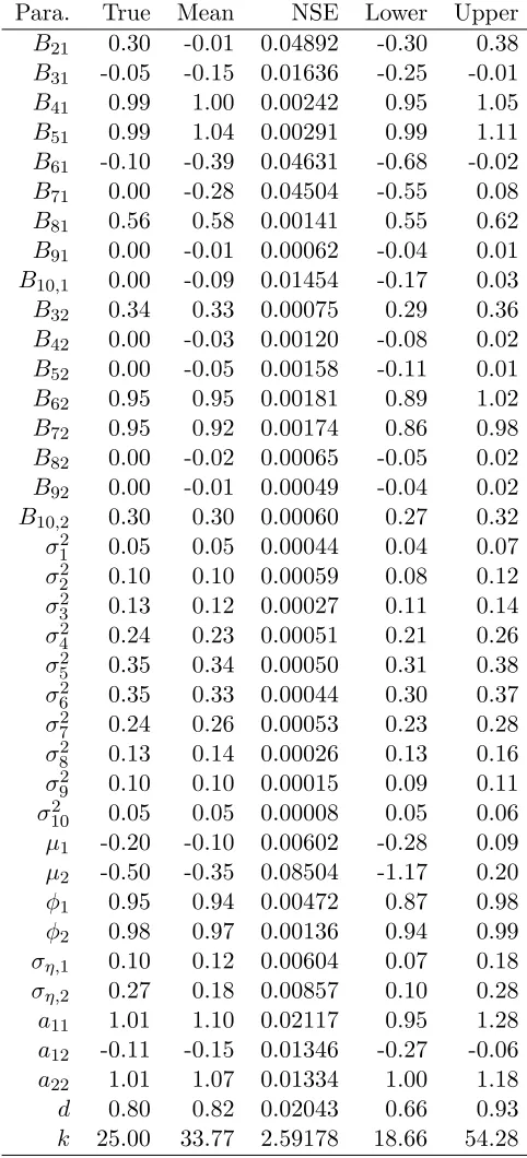
Table 3.2 Estimates for the two-factor model. . . 60

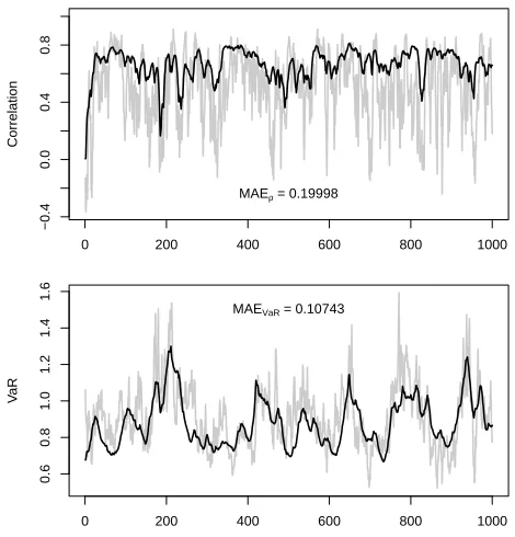
Table 3.3 MAEρ, first run. . . 68

Table 3.4 MAEρ, second run. . . 68

Table 3.5 _{MAEVaR, first run. . . .} 68

Table 3.6 _{MAEVaR, second run. . . .} 68

(9)

List of Figures

Figure 1.1 E log|Qt+1|vs. a∗21 . . . 6

Figure 1.2 Average correlation levels vs. a∗₂₁ . . . 8

Figure 1.3 Model parameters vs. Correlations in A&M’s WIC model. . . 10

Figure 1.4 logp(d|·) and the second order difference. . . 12

Figure 1.5 trA−1(logQt−1)2Qd/t−21Q −1 t Q d/2 t−1 and tr (logQt−1)2 forp= 2. . . 15

Figure 1.6 The plot of logp(k|·). . . 17

Figure 1.7 The plot of _dkd22logp(k|·) for differentp. . . 17

Figure 1.8 Dow Jones v.s. Hang Seng and Hang Seng v.s. KOSPI . . . 24

Figure 2.1 Trace plots of k and |A|from the simulation of A&M’s WIC model. . . 31

Figure 2.2 Hellinger distance between f1 andf2. . . 33

Figure 2.3 Histograms of χ2₁,χ2₂,χ2₃, and χ2₄ for non-singular Wishart. . . 36

Figure 2.4 Q-Q plots and K-S test results of χ2₁, χ2₂, χ2₃, and χ2₄ for non-singular Wishart. . . 36

Figure 2.5 Histograms of χ2 1,χ22,χ23, and χ24 for singular Wishart. . . 37

Figure 2.6 Q-Q plots and K-S test results of χ2₁,χ2₂,χ2₃, andχ2₄ for singular Wishart. 37 Figure 2.7 Histograms of χ2₁,χ2₂,χ2₃, and χ2₄ using incorrectly specifieddf. . . 38

Figure 3.1 The ten simulated observable series. . . 44

Figure 3.2 The underlying common factors and the time-varying factor correlations. 45 Figure 3.3 Trace plots of factor loadings – one-factor model. . . 54

Figure 3.4 Trace plots of idiosyncratic variances – one-factor model. . . 54

Figure 3.5 Trace plots of SV parameters – one-factor model. . . 55

Figure 3.6 Full conditionals of factor loadings – one-factor model. . . 55

Figure 3.7 Full conditionals of idiosyncratic variances – one-factor model. . . 56

Figure 3.8 Full conditionals of SV parameters – one-factor model. . . 56

Figure 3.9 Factor correlation and VaR estimates – two-factor model. . . 59

Figure 3.10 Trace plots of factor loadingsB1– two-factor model. . . 61

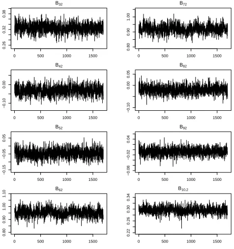
Figure 3.11 Trace plots of factor loadingsB2– two-factor model. . . 61

Figure 3.12 Trace plots of idiosyncratic variances – two-factor model. . . 62

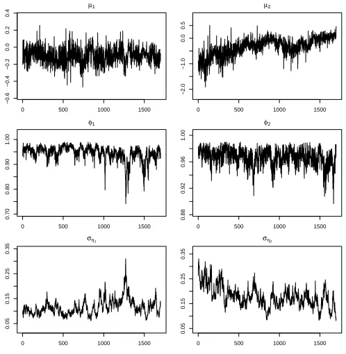
Figure 3.13 Trace plots of SV parameters – two-factor model. . . 62

Figure 3.14 Trace plots of correlation parameters – two-factor model. . . 63

Figure 3.15 Full conditionals of factor loadingsB1– two-factor model. . . 63

(10)

Figure 3.17 Full conditionals of idiosyncratic variances – two-factor model. . . 64

Figure 3.18 Full conditionals of SV parameters – two-factor model. . . 65

Figure 3.19 Full conditionals of correlation parameters – two-factor model. . . 65

Figure 3.20 Time series plot of the original data. . . 70

Figure 3.21 Factor correlations – three-factor model for real data. . . 74

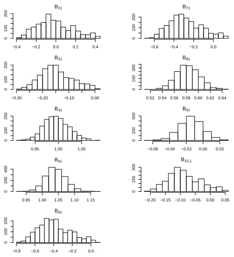
Figure 3.22 Trace plots of factor loadingsB1 – three-factor model for real data. . . . 75

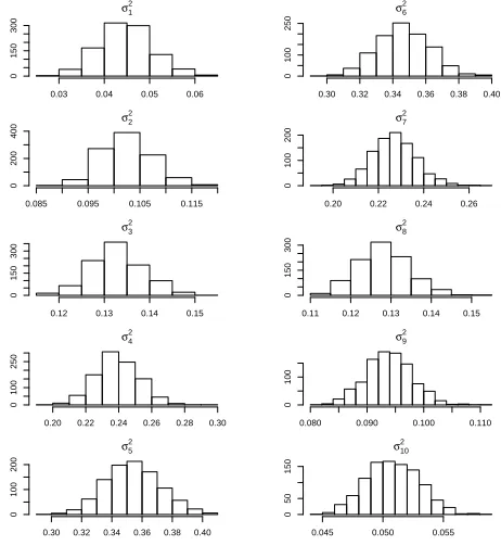
Figure 3.25 Trace plots of idiosyncratic variances – three-factor model for real data. 76 Figure 3.26 Trace plots of SV parameters – three-factor model for real data. . . 77

Figure 3.27 Trace plots of correlation parameters – three-factor model for real data. 77 Figure 3.28 Full conditionals of factor loadingsB1 – three-factor model for real data. 78 Figure 3.29 Full conditionals of factor loadingsB2 – three-factor model for real data. 78 Figure 3.30 Full conditionals of factor loadingsB3 – three-factor model for real data. 79 Figure 3.31 Full conditionals of idiosyncratic variances – three-factor model for real data. . . 79

Figure 3.32 Full conditionals of SV parameters – three-factor model for real data. . 80

Figure 3.33 Full conditionals of correlation parameters – three-factor model for real data. . . 80

(11)

Chapter 1

Modeling Dynamic Correlations in

Wishart Multivariate Stochastic

Volatility Models

1.1 Introduction

Modeling covariance and correlation structures is a central issue in financial studies and other

ar-eas. Considerable empirical evidence has shown that asset correlations are not stable over time;

this is widely known as the“correlation breakdown” phenomenon (Rey, 2000)[34]. As a result, relaxation of the correlation constancy has become essential, and the development in modeling

time-varying correlations has grown at a rapid pace. Recently, in the Multivariate Stochastic

Volatility (MSV) literature, several models have been proposed to characterize the evolution of the covariance matrices using Wishart-based processes. Gourieroux et al. (2009)[15] introduced

the Wishart autoregressive (WAR) model constructed from the scatter matrix process. Besides,

Gourieroux (2006)[14] introduced the continuous time WAR process as the direct multivariate extension of the Cox-Ingersoll-Ross (CIR) model.

Different from the WAR process of Gourieroux et al. (2009)[15], the models proposed

by Philipov and Glickman (2006; henceforth P&G)[32] and Asai and McAleer (2009; A&M hereafter)[3] adopt inverted Wishart specification for the covariance matrices. Following A&M,

this class of models is termed the “Wishart Inverse Covariance” (WIC). With this

normal-inverted Wishart setting, inference and model estimation can be implemented using Bayesian Markov chain Monte Carlo (MCMC) approaches.

The WIC models of P&G and A&M have simple structures and are proven to be useful

(12)

sensitivity parameter, A−1, are often small compared to the diagonal entries, but the

corre-sponding mean correlation estimates are quite large. This interesting phenomenon has not yet been explored in the WIC context and will be explained in the paper.

Since the WIC model for time series data is built upon latent variables and its estimation is

done through MCMC techniques, the computation is usually expensive. This is not favorable for practitioners because the model estimates may be needed to be updated on a weekly or

even daily basis. Therefore, from a practical point of view, the efficiency of the sampling

algorithm is a crucial concern. In the WIC models, both the univariate persistence parameter and the degrees of freedom (df) have complicated conditional posteriors, and hence sampling

from these densities requires additional efforts. P&G suggests a grid sampler while A&M uses

the Adaptive Rejection Metropolis Sampling (ARMS) of Gilks et al. (1995)[12]. In this article, we show that the conditional posterior densities of the above two scalar parameters are actually

log-concave, and hence the Adaptive Rejection Sampling (ARS) of Gilks (1992)[13] may be a

better alternative in this context.

Another technique to improve MCMC efficiency in the WIC model is the use of

Sherman-Morrison-Woodbury (SMW) formula. Due to the normal-inverted Wishart specification, in

the MCMC updates of the covariance matrices, we will come into a special form in which SMW formula is particularly useful. Geweke and Zhou (1996)[11] suggest using this formula

for estimating the covariance matrix of the unknown systematic factors. The main reason that they adopt SMW formula is that the inversion of a matrix can be calculated through a

much lower dimensional one. Differently, for the WIC model, the main advantage of using

SMW formula is that the update of the scale matrices for the Wishart posterior densities can be effected simply by perturbing previously computed results, and the computation is thus

reduced.

The rest of the paper is organized as follows. In Section 1.2 we explore the mechanism of how the intertemporal sensitivity parameter affects the covariance and correlation structure.

Section 1.3 discusses the implementation issue about the MCMC estimation in the WIC model.

(13)

1.2 Model Implication

We first review P&G’s and A&M’s WIC models for the p×1 asset returns yt. The model

introduced by P&G has the following simple structure:

yt|Σt∼Np(0,Σt), Σ−_t1|ν,St−1∼Wp(Σ−t1|ν,St−1),

where

St−1 =

1

νA

1

2 Σ−1

t−1

d

A12 (1.1)

is the scale parameter andν is the degrees of freedom for the Wishart distribution, respectively.

The scalardis a persistence parameter which accounts for the overall relationship. The matrix

Σt−1 is the covariance matrix of returns at time t−1, and A is the intertemporal sensitivity

parameter matrix which is symmetric and positive definite.

On the other hand, A&M’s WIC model allows for independent univariate stochastic

volatil-ity (SV) equations, which is given by

yt=Vt1/2t,

V_t1/2 = diag(eh1t/2_{, ..., e}hpt/2₎_,

ht+1=µ+φ◦ht+ηt,

where the operator◦ is the elementwise product, and

t

ηt !

ht∼N2p(0,Ut), Ut=

Pt 0

0 Pη !

.

We can see that, hit = log Var(yit|hit), i = 1, .., p, are the log volatilities of the returns, and

ht follows an first-order vector autoregressive process. For identification purpose, the diagonal

elements ofPt must be one, which meansPtis a correlation matrix. The correlation evolution

is defined by standardizing the {Qt} sequence

Pt=Q∗−t 1QtQ∗−t 1,

where

Qt= 

  

q11 · · · q1p

..

. . .. ...



(14)

is a sequence of augmented positive definite matrices, and

Q∗_t = diag(√q11, ...,√qpp).

The matrix sequence {Qt}is governed by Wishart processes, specifically,

Q−_t1|k,St−1 ∼Wp(k,St−1),

St−1 =

1

kQ

−d/2

t−1 AQ

−d/2

t−1 , (1.2)

wherekand St−1 are the df and the time-varying scale matrix parameter of the Wishart

distri-bution, respectively. The scalardis the persistence parameter, which accounts for the memory

of the {Qt} process. The matrixA is the intertemporal sensitivity parameter which is a

sym-metric positive definite matrix, and the matrixQ−_t₋d/₁2 is defined by the spectral decomposition.

One can observe that, from the settings (1.1) and (1.2), a common feature of the WIC model is that the scale matrix comes into the Wishart processes via the intertemporal sensitivity

parameterA. An interpretation of the matrix A−1 is given in A&G. As a further exploration,

we find that the A−1 also plays an important role in determining the average level of the

covariance/correlation of the asset returns, which is not discussed in both P&G’s and A&M’s

works. To provide a heuristic, yet clear explanation of how the off-diagonal elements of A−1

affect the covariance/correlation structure, in this section we solely examine the simplest case

where the number of series p = 2.Let a∗₁₁ and a∗₂₂ be the upper and lower diagonal entries of

A−1, respectively, anda∗₂₁=a∗₁₂ denote the off-diagonal elements.

1.2.1 Intertemporal Parameter and the Variance-Covariance Structures

We begin with A&M’s dynamic correlation MSV model setting (1.2). First of all, notice that

in this setting, the correlation matrix at time tis obtained by the standardization

Pt=Q∗−t 1QtQ∗−t 1,

and therefore the matrixQt can be regarded as a “covariance matrix”. By construction,

E Q−_t₊₁1 |St

=kSt=Q−td/2AQ

−d/2

t .

When k is large, the variability of the random variable becomes very small, and therefore we

are led to the approximation

(15)

By stationarity assumption, ast→ ∞,Qt→Q∞≡Q, which implies that

Q−1≈Q−d/2AQ−d/2.

This in turn gives the important approximation

Q≈ A−1

1

1−d_. _(1.3)

Approximation (1.3) refers to a large sample and large df relationship. In financial

econo-metric modelling, the number of observations tis often large. Also, in real applications, the df

kis usually large enough to make (1.3) hold good. From (1.3), fortandkbeing large, we have

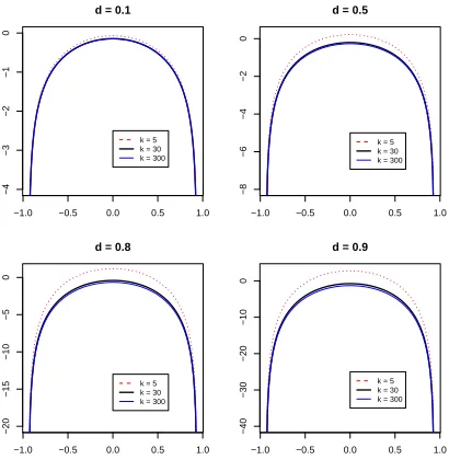
E log|Qt+1| ≈log|Q|= E log

(A−1)1−1d

= 1

1−dlog

a∗₁₁a∗₂₂−(a∗₂₁)2 .

(1.4)

Approximation (1.4) reveals that the expectation of the log-determinant of Qt+1 is a

non-linear function of a∗₂₁. We can also derive this relationship by using an autoregression (AR)

representation. Specifically, A&M’s setting implies that Qt+1 = kQd/t 2A−1/2Ξ

−1

t A−1/2Q d/2

t ,

by which we obtain

log|Qt+1|= log|kA−1|+dlog|Qt|+ log|Ξ−t1|

=

t X

j=0

log k2|A−1|

·djlog |Ξ_t−j|−1

+dt+1log|Q0|,

whereΞt

iid

∼Wm(k,I) and Q0 =I by assumption. It follows that

E log|Qt+1|=

t X

j=0

2 logk+ log|A−1|

− t X

j=0

djE log|Ξ_t−j| t→∞

= 1

1−d

2 logk−

ψ(k) +ψ(k−1) + log

a∗₁₁a∗₂₂−(a∗₂₁)2 ,

(1.5)

where ψ(·) is the digamma function. It is known that ψ(x) is asymptotically equivalent to

logx and the rate is actually very fast, e.g., when x is merely 10, we have ψ(10) = 2.25 and

log 10 = 2.30. As a result, generally,kshall be large enough such that logk≈ψ(k)≈ψ(k−1).

Taking this digamma-logarithm approximation into (1.5), the following can be derived

E log|Q| ≈ 1

1−dlog

(16)

−1.0 −0.5 0.0 0.5 1.0

−4

−3

−2

−1

0

a21

d = 0.1

k = 5 k = 30 k = 300

−1.0 −0.5 0.0 0.5 1.0

−8

−6

−4

−2

0

a21

d = 0.5

k = 5 k = 30 k = 300

−1.0 −0.5 0.0 0.5 1.0

−20

−15

−10

−5

0

d = 0.8

k = 5 k = 30 k = 300

−1.0 −0.5 0.0 0.5 1.0

−40

−30

−20

−10

0

d = 0.9

k = 5 k = 30 k = 300

Figure 1.1: E log|Qt+1|vs. a∗21

which is exactly (1.4). Figure 1.1 shows this relationship under different combinations ofdand

k. Here a∗₁₁= 0.916 and a∗₂₂= 0.953, which are taken from A&M’s result for Nikkei and Hang

Seng. Also notice that the positivity of A−1 implies that a∗₂₁ ≤ a∗₁₁a∗₂₂. It is clear that a∗₂₁

affects the expectation of the log-determinant of the covariance matrix via a nonlinear channel.

This implies that, when fitting the model, we should pay more attention to the explanation of the relationship between the return covariances/correlations and the intertemporal sensitivity

parameter. We will see this again later.

The conclusion above also applies to P&G’s WIC model. To see this, we can use a similar

argument. In the setting (1.1), for botht andν large enough, we have

Σ−∞1 ≡Σ−1 =A1/2Σ−dA1/2,

whereA1/2 is defined by Cholesky decomposition. A valid solution to this equation is

Σ=A− 1

(1−d)_,

(17)

1.2.2 Intertemporal Parameter and Correlations

Approximation (1.3) also implies how correlation structures are related to the intertemporal

sensitivity parameter. Here we illustrate the mechanism using the simplest 2×2 case. Again,

starting with A&M’s model, for a 2×2 matrix parameterA−1, by definition we can derive its

eigenvalues

λ1 =λ1(a∗₂₁) = a

∗

11+a∗22

2 +

1 2

q

(a∗₁₁−a∗₂₂)2_{+ 4(}_a∗

22)2,

λ2 =λ2(a∗₂₁) = a

∗

11+a∗22

2 −

1 2

q

(a∗₁₁−a∗₂₂)2_{+ 4(}_a∗

22)2,

and the eigenvectors

v1 =v1(a∗21) = (−a

∗

21, a

∗

11−λ1)T,

v2 =v2(a∗21) = (−a∗21, a∗11−λ2)T.

Hence, by spectral decomposition, we have the expression

A−1 1

1−d ₌

2

X

j=1

λ−_j(1−d)vjvjT

= λ

−(1−d) 1

kv1k2

a∗₂₁2 a∗₂₁(λ1−a∗₁₁)

a∗₂₁(λ1−a∗11) (λ1−a∗11)2

!

+λ

−(1−d) 2

kv2k2

a∗₂₁2 a∗₂₁(λ2−a∗₁₁)

a∗₂₁(λ2−a∗11) (λ2−a∗11)2

!

.

Now, using approximation (1.3), we can write the correlationρ as a function of a∗₂₁:

ρ≡ _p [Q]2,1

[Q]1,1[Q]2,2

(a∗₂₁)≈

L1(λ1−a∗11) +L2(λ2−a∗11)

(L1+L2)

L1(λ1−a∗11)2+L2(λ2−a∗11)2

, (1.6)

where [.]i,j is the (i, j)th entry of the matrix inside the bracket, and

L1 =L1(a∗21) =

λ−₁(1−d)

kv1k2

(a∗₂₁), L2 =L2(a∗21) =

λ−₂(1−d)

kv2k2

(a∗₂₁).

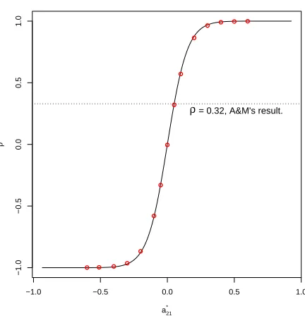
From (1.6), it is readily seen that a∗₂₁ governs the correlation structure in a nonlinear way.

Approximation (1.6) is important and useful, as it directly connects the correlation and the

intertemporal sensitivity parameter for a bivariate model. To verify this, we conduct a simula-tion study. Still, borrowing the results from Table 7(a) of A&M, we set the true parameters

d= 0.8, k = 30, A−1 = 0.916 a

∗

21 a∗₂₁ 0.953

!

.

(18)

−1.0 −0.5 0.0 0.5 1.0

−1.0

−0.5

0.0

0.5

1.0

a21

*

ρ

● ● ● ● ●

● ●

● ● ● ●

ρ = 0.32, A&M's result.

Figure 1.2: Average correlation levels vs. a∗₂₁

t= 1,2, ..., T = 500,using A&M’s WIC specification. Then, we obtain the correlation matrices

Pt by applying the standardization procedure given in A&M’s formula (4). Finally, for each

a∗₂₁,we calculate the mean sample correlations

¯ ˆ

ρ= 1

T

T X

t=1

[Pt]2,1.

The relationship implied by (1.6) can therefore be verified by comparing the theoretical and the sample values. Figure 1.2 shows the simulation results. The red circles are the mean sample

correlations and the solid curve is the theoretical ρ given by (1.6). We can see that the red

circles are all located on the curve, which means that the relationship between the correlation and the intertemporal sensitivity parameter can be well explained by (1.6). From Figure 1.2 we

can also observe that, whena∗₂₁ = 0.05,all the parameters are approximately the same as the

model estimates in Table 7(a) of A&M; in this case, the mean sample correlation is about 0.3, which coincides the average level of the correlation estimates given in Figure 3 of A&M. This

further verifies the plausibility of (1.6). Since all the above results can also be derived from

P&G’s setup in a parallel manner, equation (1.6) also applies to P&G’s WIC model.

One should also notice that, in the WIC model, due to the nonlinear relationship, a small

(19)

to be very careful in explaining the estimation results. For instance, in Figure 1.2, a∗₂₁ = 0.05

implies a modest correlation (which equals to 0.3). Whena∗₂₁ is changed from 0.05 to 0.1, this

increment looks small and we might think it makes no difference; however, in fact, it leads the

correlation to jump from 0.3 to 0.5, which can be regarded as a fairly strong correlation.

1.2.3 Model Parameters vs. Correlation

For the WIC models, the model form does not clearly reveal the relationship between the parameters and the correlations. To study the question, in this section we conduct a visual

analysis using A&M’s model with two-dimensional simulated data. For each parameter we set two very different values so that by contrast we can observe how the correlation behavior is

governed by the parameters. Specifically, the data generating process (DGP) are given by

h1,t+1= 0.98h1t+η1t,

h2,t+1= 0.95h2t+η2t,

η1t

η2t !

∼N

"

0

#

,

"

0.1662 ₀

0 0.2602

#!

, and vt= (v1t, v2t)0 ∼N(0,Pt),

where Pt, as defined previously, is the correlation matrix obtained by standardization of Qt.

For the correlation level, let A−1₂_,₁=a∗ and set the parameters of interest as

a∗_H = 0.10, dH = 0.95, kH = 100;

a∗_L= 0.02, dL= 0.05, kL= 5.

It is obvious that the difference in the settings ofdandkare large, whereas for a∗ it may seem

small. However, recall in last section we have shown that the mean level of the correlation

is highly nonlinear in the off-diagonal elements of A−1, and therefore the difference between

a∗ = 0.02 and a∗ = 0.10 shall be large enough to simulate very different correlation patterns.

As each parameter has two levels, we have 23 = 8 combinations in total. For one combination

we simulate a sample of sizeT = 500. Figure 1.3 shows the simulated data.

It is quite clear that the correlation patterns are so different under different settings. Let’s

begin with the role ofa∗, which is explored in detail in Section 1.2. We can find that, givendand

k held equal, a∗ determines the average level of the correlation. This is particularly apparent

in the bottom four graphs of Figure 1.3 where the correlations appear to be constant. When

a∗= 0.1, the mean correlation is approximately 0.1, whilea∗ = 0.02, the mean correlation level

goes down to as low as 0. This pattern is consistent with what we showed in last section. Next,

(20)

0 200 400 600 800 1000

0.0

0.4

0.8

a* = 0.1 , d = 0.95 , k = 100

0 200 400 600 800 1000

−0.5

0.0

0.5

1.0

a* = 0.1 , d = 0.95 , k = 5

0 200 400 600 800 1000

−0.3

0.0

0.2

0.4

a* = 0.1 , d = 0.05 , k = 100

0 200 400 600 800 1000

−1.0

0.0

1.0

a* = 0.1 , d = 0.05 , k = 5

0 200 400 600 800 1000

−0.5

0.0

0.5

a* = 0.02 , d = 0.95 , k = 100

0 200 400 600 800 1000

−1.0

0.0

1.0

a* = 0.02 , d = 0.95 , k = 5

0 200 400 600 800 1000

−0.3

0.0

0.2

a* = 0.02 , d = 0.05 , k = 100

0 200 400 600 800 1000

−1.0

0.0

1.0

a* = 0.02 , d = 0.05 , k = 5

Figure 1.3: Model parameters vs. Correlations in A&M’s WIC model.

correlations. Finally, we can obviously see that d controls the persistence of the correlations

across time, which has been well explained in P&G and A&M.

1.3 MCMC Estimation

This section focuses on the MCMC implementation issue in the WIC models. Some general problems are explored. The first is the efficiency, a major concern when applying MCMC

methodology. We show that, although looking complicated, the posterior densities of the per-sistence parameter and the df parameter are log-concave. Consequently, instead of using ARMS,

we can apply ARS to draw samples in each MCMC sweep. There are two advantages of using

(21)

to perform the Metropolis step, and secondly, we can construct squeezing functions, which

may save function evaluations in each rejection step. Compared to grid sampler, ARS is more efficient and accurate. In addition to the improvement in sampling procedures, we suggest

exploiting SMW formula in updating the covariance matrices; later we will see that the use

of ARS together with SMW formula can significantly improve MCMC efficiency. The other concern in the WIC model is the choice of priors for the df parameter, as the posterior density

is diffuse and accordingly, the estimation would be sensitive to the prior. Finally, P&G and

A&M use different parameterizations for the scale matrix in the Wishart distribution. It is then natural to ask if one formulation is superior than the other. These questions are also studied

in this section.

1.3.1 Likelihoods and Joint Posteriors

In P&G’s model with setting (1.1), the likelihood function is given by

L(A, d, ν|y)∝ T Y

t=1

Wp(Σ−t1|ν,St−1)Np(yt|Σt)

∝ T Y

t=1

|Σ−_t1|1/2exp

−1 2y T tΣ −1

t yt

×|S −1

t−1|

ν

2|Σ−1

t | ν−p−1

2

2νp2 Γ_p(ν)

exp

−1

2tr S

−1

t−1Σ

−1

t

,

where y = {yt} and Γp(ν) =

Qp

i=1Γ [(ν−i+ 1)/2] with Γ(·) being the gamma function. On

the other hand, for A&M’s model where the independent SV equations are introduced, the estimation requires little more effort. A&M proposed a two-stage estimation procedure. In the

first stage, for the ith series, the errors t are obtained by the standardization t = V

−1/2

t yt,

and in the second stage, we then have the similar likelihood function forA,d, and k:

L(A, d, k|)∝ T Y

t=1

Wp(Q−t1|k,St−1)Np(t|Pt)

∝ T Y

t=1

|P_t−1|1/2_exp

−1

2

T tPt−1t

×|S −1

t−1|

k

2|Q−1

t | k−p−1

2

2kp2 Γ_p(k)

exp

−1

2tr S

−1

t−1Q

−1

t

,

where = {t} and Γp(k) has the same definition as the above. Since the joint posterior is

(22)

−1.0 −0.5 0.0 0.5 1.0 −20000 −10000 d log poster ior

p = 2

−1.0 −0.5 0.0 0.5 1.0

−3.0

−2.0

−1.0

d

2nd Order Diff

erence

Maximum = −0.87

−1.0 −0.5 0.0 0.5 1.0

−60000

0

d

log poster

ior

p = 3

−1.0 −0.5 0.0 0.5 1.0

−150

−100

−50

0

d

2nd Order Diff

erence

Maximum = −0.5

−1.0 −0.5 0.0 0.5 1.0

−1e+05

0e+00

d

log poster

ior

p = 4

−1.0 −0.5 0.0 0.5 1.0

−400

−200

0

d

2nd Order Diff

erence

Maximum = −0.82

Figure 1.4: logp(d|·) and the second order difference.

1.3.2 Log-concavity of the Full Conditional of d

The conditional posteriorp(d|·) in P&G’s model is of exactly the same form as that in A&M’s.

Here we adopt A&M’s notation. Given a uniform (-1,1) prior, the posterior density has the form

p(d|·)∝exp

ζd−1

2tr

A−1C−1(d)

I(−1,1)(d),

where ζ = −(k/2)PT

t=1log

Q−_t₋1₁

and C−1(d) = k PT

t=1Q

d/2

t−1Q

−1

t Q d/2

t−1. Before proving

log-concavity, we would like to examine the behavior of logp(d|·). Figure 1.4 shows the log posterior

density function ofdand its second order difference as a discrete approximation for _∂d∂22logp(d|·).

The data are simulated from d= 0.8, k = 10, and several arbitrarily chosen A−1. It is very

clear that, for each p, logp(d|·) presents a concave shape and the second order difference is

negative throughout the support (-1,1). This simulation provides convincing visual evidence

for concavity of logp(d|·).

Now, note that, in the log posterior density, the first termζ =−k₂PT

t=1log|Q

−1

(23)

of d. It vanishes after taking differentiation. The second order derivative is then given by

∂2

∂d2logp(d|·) =−

1 2

T X

t=1

trA−1(logQt−1)2Qd/_t−21Q

−1

t Q d/2

t−1

+ 2A−1/2(logQt−1)Qd/t−21Q

−1

t Q d/2

t−1(logQt−1)A−1/2

+Qd/_t₋2₁Q−_t1Qd/_t₋2₁(logQt−1)2A−1

.

(1.7)

Our task boils down to showing that (1.7) is non-positive. SinceA−1/2(logQt−1) is non-singular

andQd/_t₋2₁Q_t−1Qd/_t₋2₁is symmetric and positive definite, the middle term of the summand in (1.7)

is positive definite and thus has a positive trace. Next we would like to explain why the first and the third terms of the summand have nonnegative traces. Since the third term is just the

transpose of the first one, we only need to show that the first matrix product is of nonnegative

trace.

Intuitively, we may want to show that it is positive or nonnegative definite; unfortunately,

this is a stronger result and could be very difficult to prove. A heuristic way is to apply the

expectation equation

EQd/_t₋2₁Q_t−1Qd/_t₋2₁=A,

and by substitution we obtain

Rt≡tr

A−1(logQt−1)2Qd/_t−21Q

−1

t Q d/2

t−1

≈trA−1(logQt−1)2A = tr

(logQt−1)2 >0,

(1.8)

since (logQt−1)2 is positive definite.

In addition to the expectation argument, we may verify the trace nonnegativity from an

eigen decomposition point of view. To see this, taking a simple 2×2 case as an example,

suppose that

A−1 = 1 c

c 1

!

; (1.9)

apparently, forc= 0, the matrixA−1 is an identity and thus both its two eigenvalues are equal

to 1. In this case,Rt is reduced to tr

(logQt−1)2Qd/_t−21Q

−1

t Q d/2

t−1 ≥0 since the product of two

real-symmetric positive definite matrices has a nonnegative trace.

For another extreme case where c→ ±1, the matrixA−1 will be nearly singular; therefore,

the larger eigenvalue will dominate the other. Our argument is, by letting cchange from−1 to

1, we are in fact going over all possibilities of A−1 from one extreme, the identity matrix, to

another, which is a nearly singular matrix. Consequently, if under all these situations Rt ≥0,

(24)

thus (1.7) is positive.

With simulation, Figure 1.5 presents graphic explanations of the expectation argument

stated in (1.8) and the eigen decomposition argument. The sample size is T = 1000, and the

parameters d= 0.8, k= 10; the matrixA−1 is set according to the form given by (1.9).

Top-left, top-right, and bottom-left are the time-series plots for the element c=−0.99, 0, and 0.99,

respectively, where the grey line is the plot ofRt= tr

A−1(logQt−1)2Qd/t−21Q

−1

t Q d/2

t−1 and the

black line is tr(logQt−1)2 . It is readily seen that the two traces are actually positive for allt,

and the mean levels ofRtand of tr

(logQt−1)2 are indeed about the same, althoughRtis more

volatile. As c marches away from zero, i.e. A−1 gets nearly singular,Rt and tr

(logQt−1)2

become more positive. On the other hand, when c = 0, which means A−1 is an identity, the

two traces are both small positive numbers. In any case, it is evident that mean Rt ≈ mean

tr

(logQt−1)2 ≥0. This verifies the plausibility of using (1.8) to hypothesize trace positivity.

Bottom-right is the plot of meanRtover allc∈(−0.99,0.99). The curve is above 0 for every

c, which is a strong evidence of nonnegativity ofRt. Also, the smile shape reflects the fact that

we just mentioned: as A−1 becomes nearly singular, the trace Rt will be more positive, and

vice versa. The reason whyRtis guaranteed to be nonnegative is complicated and unclear, and

this is why it is demonstrated numerically. One may argue that, it is possible that Rt <0 for

some time pointst, but we have to point out that, we never see this happen empirically. Even

if someRt<0, though never happened to us, it will not change positivity of the summand in

(1.7) since the trace sums upRtover allt. The majority ofRt>0 will offset those negativeRt,

if any. Moreover, remember that in (1.7), the second term of the summand is strictly positive,

(25)

0 200 400 600 800

0

500

1000

1500

Time c = −0.99

0 200 400 600 800

0

5

10

20

30

Time c = 0

0 200 400 600 800

0

500

1000

Time c = 0.99

●

● ● ● ●_● ●●●

●●●●●●●●●●●●●●●●●●●●●●●●●●●●●●●●●●●●●●●●●●●●●●●●●●●●●●●●●●●●●●●●●●●●●●●●●●●●●●●●●●●●●●●●●●●●●●●●●●●●●●●●●●●●●●●●●●●●●●●●●●●●●●●●●●●●●●●●●●●●●●●●●●●●●●●●●●●●●●●●●●●●●●●●●●●●●●●●●●●●●● ●●● ● ● ● ●

−1.0 −0.5 0.0 0.5 1.0

0

100

300

500

c

Mean T

race

c∈∈(−0.99, 0.99)

Figure 1.5: trA−1(logQt−1)2Qd/_t−21Q

−1

t Q d/2

t−1 and tr

(logQt−1)2 forp= 2.

1.3.3 Log-concavity of the Full Conditional of k

The full conditionals ofkin P&G and in A&M merely differ in the prior part. We can observe

that the prior used in A&M is a special case of that in P&G with the location parameter α

chosen to be 1. In practice, we shall choose α ≥ 1 so that the mass of the density will not

gather up close to zero. To give a unified discussion, we start with the gamma prior having the form:

π(k) = exp(α−1) logk−βk , α≥1, k > p.

(26)

the posterior density ofk is then

p(k|·)∝exp

(α−1) logk−βk+T kp

2 log(k/2)−

T k

2 log|A| −T

p X

j=1

log Γ

k+ 1−j

2 ×exp k 2 T X t=1

logQ

d/2

t−1Q

−1

t Q d/2

t−1

−

1

2tr

A−1C−1(k)

.

where C−1(k) = kPT

t=1Q

d/2

t−1Q

−1

t Q d/2

t−1 is the same as C−1 defined previously. In deriving

log-concavity of the full conditional of k, the main difficulty lies in the gamma function. For

the gamma component, letzj ≡ k+1₂−j, we have

d2

dk2 log Γ(zj) =

1

4ψ1(zj),

where ψ1(zj) is the trigamma function. Using the fact that the trigamma function is strictly

decreasing in its argument and k₂ ≥zj,forj= 1, ..., p, we obtain

ψ1

k

2

≤ψ1(zj).

Therefore, the second order derivative of the log conditional posterior is

d2

dk2logp(k|·) =

1 4T p2 k− p X j=1

ψ1(zj)−

α−1

k2

≤ 1

4T p

2

k−ψ1

k

2

− α−1

pk2

.

To complete the proof, we need to show that 2/k−ψ1(k/2)≤0. Takingx=k/2>0,and

applying the inequality (Choi and Wette, 1969)[6]

1

x < ψ1(x),

the result immediately follows. Figure 1.6 is the plot of logp(k|·), which is generated from

simulated data with the mode equal to 30. Figure 1.7 shows the second order derivatives of

(27)

0 20 40 60 80 100

−1000

−500

0

k

log poster

ior

Figure 1.6: The plot of logp(k|·).

0 20 40 60 80 100

−257.7

−257.5

−257.3

p = 2

k

0 20 40 60 80 100

−235.6

−235.4

−235.2

p = 3

k

0 20 40 60 80 100

−219.6

−219.4

−219.2

p = 4

k

0 20 40 60 80 100

−207.1

−206.9

−206.7

p = 5

k

(28)

1.3.4 Use of Sherman-Morrison-Woodbury Formula

In the estimation for the WIC model, we need to update the covariance matrices in each

iteration. The conditional posterior of the inverted covariance matrix is proportional to a

Wishart distribution with the scale matrix

˜

St−1 = St−−11+xtx0t −1

, t= 1, ..., T,

wherextis the mean-corrected return vector in P&G’s model, while in A&M’s model, it denotes

the series filtered by the univariate stochastic volatility equations.

If we apply SMW formula, the scale matrixS˜t−1 is calculated by

S_t−₋1₁+xtx0t −1

=St−1−

St−1xtx0tSt−1

1 +x0_tSt−1xt

.

Since in each sweep,St−1is known from previous iteration, we can obtainS˜t−1by rank-1 update

rather than by matrix inversion from scratch. Obviously, this is computationally cheaper and hence should be incorporated into the MCMC algorithm.

1.3.5 Hyperparameter Assessment for the Degrees of Freedom

Choosing priors for df is important in the WIC model. We find that, from empirical experience,

the conditional posterior density of df is generally diffuse. We have seen the log posterior of k

in Figure 1.6. It is not hard to see that the density is quite diffuse. Therefore, the inference

is easily affected by the priors. P&G suggest a gamma prior, while A&M adopt the

exponen-tial distribution. However, both P&G and A&M do not mention how to choose reasonable hyperparameters, which is, as a matter of fact, really essential in the model estimation.

As discussed in Section 1.3.3, for the gamma prior used in P&G, we should chooseα≥1 for

practical purposes. The problem is then simplified to the shape. Since the inference is sensitive to the prior distribution, we may want to choose a vague prior to avoid the dominance from

subjective information. This means that we should set hyperparameters regarding the shapes

which can give reasonably flat priors. Our experience suggests that, for β in P&G and λ0 in

A&M, 0.1 to 0.5 would be a reasonable range for these hyperparameters.

1.3.6 The Scale Matrix of the Wishart Distribution

A&M point out that we can possibly use the parameterization

St=

1

k(A

1/2₎₍_Q−1

t−1)

(29)

Table 1.1: Mean absolute error of correlation estimates using different specifications.

DGP

Spec. A&M P&G

A&M 0.1680 0.1727

P&G 0.2027 0.1976

Table 1.2: Mean absolute error of VaR using different specifications.

DGP

Spec. A&M P&G

A&M 0.2204 0.2217

P&G 0.2156 0.2182

where A1/2 is defined by Cholesky decomposition. Actually, this is the specification adopted

in P&G’s model. Some questions arise here: what if the “true” DGP is from one specification

but we use the other to fit the data? Does one specification outperform the other under all circumstances? These questions are the main interests in this section.

We compare the two specifications (1.2) and (1.8) using the setting below

h1,t+1= 0.98h1t+η1t, ση1 = 0.166,

h2,t+1= 0.95h2t+η2t, ση2 = 0.260,

A−1 = 1.0 0.1

0.1 1.0

!

, d= 0.8, k = 30.

Two datasets, each with 1000 observations, are generated using (1.2), A&M’s specification,

and (1.8), P&G’s, respectively. Following A&M, the comparison is effected according to two

performance measures based on mean absolute errors (MAE), namely MAEρ and MAEVaR,

which are also defined in A&M Section 3.4. Table 1.1 shows MAEρ results. We can see

that the model with A&M specification has smaller MAE no matter what the true DGP is.

However, as shown in Table 1.2, when MAEVaR is used as the criterion, the model with P&G

specification performs better for both true DGPs. Moreover, we can observe that the mean

(30)

1.4 Empirical Study

This section presents a real data application as an illustration of our findings. The dataset,

obtained from Yahoo Finance, contains four series of stock market index returns, namely Dow Jones Industrial Average (DJIA), Hang Seng Index (Hang Seng, HSI), Korea Composite Stock

Price Index (KOSPI), and Taiwan Weighted Stock Index (TAI). The sample period for all series

is 2 July 1997 to 9 November 2009, giving a total T = 452 observations. Following A&M, the

return series are defined as 100×(logPit−logPi,t−1), where Pit is the closing price on week

t for stock market i. The data are fitted with A&M’s model and the study is conducted as

follows.

1.4.1 Improving MCMC Efficiency

The primary interest of this empirical study lies in whether ARS together with SMW formula

can improve MCMC efficiency. First, we estimate the model using ARS plus SMW formula. We denote this by “ARS + SMW.” Then, on the other hand, the model is estimated using

ARMS and usual matrix inversion. This combination is denoted by “ARMS + No SMW. By

comparing these two schemes, we know how much time is saved. For each combination, we run the estimation procedures two times and then take the average time consumed. The OX[8]

programs are run with OX Console version 5.10 on Windows Vista platform, on a machine

equipped with an Intel Core2 Duo 8400 3.0 GHz central processing unit (CPU) and 8 gigabytes random access memory.

Table 1.3 shows the average time used in each combination. We see that, time used in

ARMS + No SMW is more than that in ARS + SMW by 380.12 seconds, which equals to a 12% difference. Evidently this is a considerable improvement. Moreover, as one can expect,

using SMW formula will be more advantageous as the dimension of data increases since the

complexity of usual matrix inversion is growing faster than O(p2_).

Next, we examine the MCMC estimates from the combinations ARS+SMW and ARMS

+ No SMW. Notice that here we do not show the fitting results of the univariate stochastic

volatility models since they are not of the main interest. The number of iterations isN =M+L.

The first M draws are discarded and the remaining L are kept for inference. We output the

posterior means, the numerical standard errors (NSE) of the posterior means, the 95% intervals, the relative numerical efficiency (RNE), and the p-values of the convergence diagnostic (CD)

statistics introduced by Geweke (1992)[10]. The NSEs and RNEs are calculated by the function

“numEff” of the R package “bayesm” developed by Rossi, Allenby, and McCulloch (2005)[35],

which use a Bartlett window with a bandwidth of 0.1·L. The 95% intervals are obtained by

the (2.5th, 97.5th) percentiles of the L draws. To be consistent with the NSEs and RNEs,

(31)

the analysis, we use N=20,000 andM=10,000, producing a final sample of size L=10,000. As

mentioned in Section 1.3.3, since the posterior of the df parameter is diffuse, we choose the

hyperparameter λ0 = 0.2. The MCMC estimation results are shown in Table 1.4 and Table

1.5, respectively. First note that the estimated d is about 0.4 with significance, implying a

time-varying correlation structure. We can see that the estimation results are quite similar,

with some minor differences inA. In summary, for the two schemes generate similar estimates,

we would prefer ARS+SMW since it is more efficient.

Table 1.3: Comparison results of ARS+SMW v.s. ARMS+No SMW.

Combination Time Elapsed (Sec.)

ARS+SMW 3248.64

(32)

Table 1.4: Output of ARS + SMW .

Parameter MEAN NSE 95% Interval RNE CD

a11 1.470 0.11433 (0.796, 2.232) 858.259 0.088

a12 -0.313 0.01210 (-0.452, -0.220) 441.382 0.110

a13 -0.155 0.01019 (-0.283, -0.072) 361.562 0.254

a14 -0.050 0.00379 (-0.137, 0.020) 95.852 0.598

a22 1.108 0.03025 (0.896, 1.308) 674.911 0.052

a23 -0.250 0.01134 (-0.372, -0.155) 409.336 0.124

a24 -0.236 0.00684 (-0.319, -0.160) 273.265 0.154

a33 1.224 0.08610 (0.626, 1.739) 848.412 0.054

a34 -0.269 0.00945 (-0.389, -0.184) 350.349 0.132

a44 1.073 0.03162 (0.859, 1.408) 575.371 0.146

d 0.445 0.01626 (0.308, 0.582) 509.448 0.168

k 11.646 0.30471 (9.548, 14.577) 490.044 0.134

Table 1.5: Output of ARMS + No SMW.

a11 0.792 0.03435 (0.569, 1.079) 636.497 0.060

a12 -0.288 0.01762 (-0.433, -0.165) 542.064 0.256

a13 -0.129 0.00425 (-0.196, -0.079) 191.593 0.372

a14 -0.056 0.00365 (-0.114, -0.006) 179.123 0.300

a22 1.683 0.06430 (1.312, 2.206) 647.406 0.058

a23 -0.271 0.01778 (-0.438, -0.139) 512.682 0.208

a24 -0.242 0.01241 (-0.387, -0.135) 378.197 0.148

a33 0.989 0.03705 (0.800, 1.437) 580.692 0.094

a34 -0.233 0.00993 (-0.357, -0.158) 402.822 0.124

a44 0.861 0.03718 (0.597, 1.125) 629.172 0.098

d 0.407 0.02789 (0.207, 0.621) 630.867 0.068

(33)

1.4.2 Marginal v.s. Joint Behaviors

In this section, we examine the marginal bivariate model estimations. Table 1.6 gives the

Pearson correlations of the four stock market return series. We can observe that, among the

selected Asian markets, HSI has the highest correlation with DJIA. Hence, the DJIA-HSI pair can be used as the representative for studying American-Asian stock markets. Also, in the

Asian markets, the HSI-KOSPI pair has highest correlation and hence we use it to study Asian

markets. The bivariate models for the two pairs are estimated using MCMC method with

N = 20000 iterations. The first 8000 draws are discarded and the next 12000 are recorded.

The estimates for the two models are given in Table 1.7 and Table 1.8. First of all, notice

that, since in the bivariate case we can study the relationship between A−1 and the mean

sample correlations, we output the estimates fora∗_ij = [A−1]ij instead of the estimates for aij.

From Table 1.7 and 1.8, we find it interesting that, for the DJIA-HSI model, the persistence parameter is approximately 0 (the 95% interval widely covers 0), which indicates a constant

correlation by the WIC model implication. This result is different from those shown in Table

1.4 and 1.5, where a dynamic correlation structure is revealed. Moreover, the estimate for the

df parameter k also varies quite a bit in different cases. For the DJIA-HSI bivariate model, k

is merely 8, while for the HSI-KOSPI pair, k has been doubled to 16. More interestingly, the

estimate for k from the full model is in between the two bivariate models. This phenomenon

is different from the discovery in A&M, in which the estimate ofk is larger for the full model

than for all marginal bivariate models. Our explanation is that, the full model is a joint of the

marginal models; consequently, what it presents is the compromise among all different bivariate relationships.

We are also interested in the relationship between the average sample correlations and the

intertemporal sensitivity parameter matrixA−1. These relationships are shown in Figure 1.8.

In the left-hand side plots, the black curves are the function values ofρ(a∗₁₂) given by (1.5) and

the red circles are the “predicted” correlations given the estimates of a∗₁₂. On the right hand

side are the mean sample correlations. We can see that, for the DJIA-HSI bivariate model,

the black curve is a little bit convex, as dis slightly negative (however, we have to emphasize

that it is not statistically different from 0). It is then obviously seen that, because of the zero

persistence, the correlations are shown to be constant. The red circle is exactly located on the black curve, which means that the behavior of the correlations is well captured by equation

(1.5). More importantly, we find that, for the estimate ofa∗₁₂= 1.13, the “predicted” correlation

ρ(a∗₁₂) is about 0.55, which approximately equals to the mean level of the sample correlations

between DJIA and HSI.

On the other hand, for the HSI-KOSPI model, the black curve is slightly concave since

(34)

0.0 0.5 1.0 1.5

0.0

0.2

0.4

0.6

0.8

1.0

a₂₁*

ρρ

((

a21

*))

DJIA − HSI pair

●

Time

0 100 200 300 400

0.0

0.2

0.4

0.6

0.8

Dow Jones v.s. Hang Seng

0.0 0.2 0.4 0.6 0.8

0.0

0.2

0.4

0.6

0.8

1.0

a₂₁*

ρρ

((

a21

*))

HSI − KOSPI pair

●

Time

0 100 200 300 400

0.0

0.2

0.4

0.6

0.8

Hang Seng v.s. KOSPI

Figure 1.8: Dow Jones v.s. Hang Seng and Hang Seng v.s. KOSPI

aggregate, the correlations present a constant pattern, but with a careful examination, it is not

hard to find that, actually, the correlations mildly change over time. Like the DJIA-HSI case,

the red circle is perfectly located on the black curve; this again supports the plausibility of

equation (1.5). Likewise, we can observe that, for the estimate of a∗₁₂ = 0.51, the “predicted”

correlation ρ(a∗₁₂) is 0.6, which is about the average level of the sample correlations between

HSI and KOSPI.

The results from the DJIA-HSI and the HSI-KOSPI bivariate models provide empirical

evidence supporting the plausibility of equation (1.5). This also suggests the importance and

practical usefulness of (1.5). We can use this relationship between the correlations and A−1

implied in the marginal bivariate models as a diagnostic check for model adequacy. Specifically,

if the model is fitted correctly, then the values ofρ(a∗₁₂) obtained from the estimateda∗₁₂ should

(35)

Table 1.6: Pearson correlations of the four return series.

DJIA HSI KOSPI TAI

DJIA 1.000

HSI 0.553 1.000

KOSPI 0.420 0.566 1.000

TAI 0.370 0.531 0.486 1.000

Table 1.7: DJIA-HSI bivariate model estimates.

a∗₁₁ 1.491 0.205 (0.654, 3.633) 769.739 0.134

a∗₁₂ 1.130 0.094 (0.500, 2.219) 553.129 0.232

a∗₂₂ 2.178 0.209 (0.863, 4.652) 701.532 0.082

d -0.194 0.076 (-0.592, 0.353) 862.296 0.129

k 16.231 1.513 (6.282, 34.595) 427.914 0.294

Table 1.8: HSI-KOSPI bivariate model estimates.

a∗₁₁ 0.636 0.021 (0.448, 0.878) 408.424 0.434

a∗₁₂ 0.505 0.040 (0.233, 0.967) 516.407 0.260

a∗₂₂ 1.476 0.153 (0.729, 3.220) 631.708 0.102

d 0.138 0.050 (-0.294, 0.566) 548.086 0.134

(36)

1.5 Conclusion

In this paper we give a general discussion of the WIC model proposed by P&G and A&M.

We first derive the relationships between the intertemporal sensitivity parameter A−1 and

the covariance/correlation structures in the bivariate cases. This reveals the fact that the

off-diagonal entries ofA−1affect the covariances/correlations through a nonlinear channel. We then

show log-concavity of the univariate posterior densities of the persistence parameter and the df parameter. With log-concavity being assured, we can use ARS as a more efficient sampling

scheme for the MCMC inference. Moreover, we suggest adopting SMW formula in the update of

correlation matrices. This also helps improving MCMC efficiency. Also, we suggest reasonable

values for the hyperparameters α and β for the prior distributions of the df parameter. The

final topic is about the parameterizations used by P&G and A&M. Our simulation study shows that it does not matter which parameterization to use. Both are equally reasonable.

We give an empirical data analysis as a demonstration of our findings. In this study we show

that ARS together with SMW can considerably improve sampling efficiency and hence should be used in the estimation of the WIC model. Marginal bivariate models are also discussed. The

results show that the joint behavior of the series in the full model may be different from the

(37)

Chapter 2

On Random Wishart Matrices

2.1 Introduction

Asset correlations are well known to be unstable over time. Therefore, in financial modelling, capturing the dynamic covariance and correlation structure has become a central issue. In the

literature of Multivariate Stochastic Volatility (MSV), several recently proposed models suggest

using Wishart processes to characterize the evolution of covariance matrices. For example, Philipov and Glickman (2006)[32] and Asai and McAleer (2009; henceforth A&M)[3] adopt an

inverse Wishart specification for the covariance matrices, so that statistical inference and model

estimation can be effected through Bayesian Markov chain Monte Carlo (MCMC) methods. Following A&M, this class of models is termed the “Wishart Inverse Covariance” (WIC), and

the Wishart distribution is denotedWp(k,S), wherekis the degrees of freedom (df) parameter,

S is the scale matrix, andp is the dimension ofS.

Since the WIC model for time series data is built upon latent variables and its estimation

relies on MCMC approaches, the computation is expensive. To deal with this type of model, OX[8] would be an ideal choice, as it is fast and it has extensive and well developed packages for

Bayesian inference. A problem arises here: in A&M’s model settings, k is not restricted to be

integer-valued; it could be fractional (non-integer). However, the generation of random Wishart

matrices with a fractionalkis not available in OX. The existing OX function “ranwishart” will

simply take the floor value of any fractional kas the input argument and thus the matrix that

has been sampled is in fact from a Wishart distribution with a integer-valued k, which is not

correct. In such cases, our simulation studies in this chapter show that the estimation will be

seriously misled. To fix the problem in OX, we develop the Wishart package, “WishPack”, in

which fractional df are considered.

One thing to emphasize here is that, by the fact known as Gyndikin’s theorem (see, e.g.,

(38)

and non-integer; nevertheless, most existing statistical software packages set the restriction that

k≥p, which is not appropriate and does not cover all possibilities. There is one more drawback

implied in this restriction. Whenkis integer-valued and 0< k < p, the Wishart matrix is known

to be almost surely singular (Uhlig, 1997)[40] and is still well defined. The singular Wishart

matrix can be generated via fairly simple procedures and has shown to be useful in practical

problems, e.g. Konno (2009)[23]. However, with the restriction k ≥ p, generating singular

Wishart matrices becomes impracticable. In summary, according to Gyndikin’s theorem, it is

valid to generate random Wishart matrices with anykbelonging to the Gyndikin set{1,2, ..., p−

1} ∪(p−1,∞), but unfortunately, existent statistical packages such as Matlab “MCMC”[38],

OX, R “MCMCpack”[29], SAS[36], etc., do not treat the generation of random Wishart matrices

in this manner and are therefore incomplete. To correct these mistakes, Wishpack is developed based on Gyndikin’s theorem. This feature has not yet been seen in other statistical packages.

In the recent past, there has been a number of studies of singular Wishart distributions.

The probability density function with respect to Lebesgue measure on an appropriate space is explicitly given by Srivastava (2003)[39]. Practical uses of singular Wishart distributions are

discussed in Uhlig (1997)[40] and Kubokawa and Srivastava (2008)[24], among others. In

re-sponse to those needs, Wishpack also takes into account the singular Wishart densities. Finally, as a parallel product, Wishpack also provides an inverse Wishart generator with fractional df,

and the density function of the inverse Wishart distribution.

The rest of the chapter is organized as follows. In Section 2.2 we motivate the generation

of Wishart matrices with fractional df. The generation of the singular Wishart matrix is also

discussed. Section 2.3 illustrates the algorithm for generating Wishart random matrices with

fractional df by applying Bartlett’s decomposition. A short discussion of another popular

variant, namely the Odell-Feiveson’s (1966)[30] algorithm, is given as well. Some concluding

remarks are summarized in Section 2.4.

2.2 Motivation

Gyndikin’s Theorem (the real matrix case):

Following Graczyk et al. (2003)[16], letV be a positive definite matrix of sizep×pand Θbe

an appropriate symmetricp×pmatrix. Suppose we have i.i.d. random vectorsXi ∼Np(0,V),

then the scatter matrixW = 1₂Pk

i=1XiXiT has the Laplace transform

Ehetr(ΘW)i= [det(Ip−VΘ)]−k.

The set of values ofksuch that [det(Ip−VΘ)]−kis the Laplace transform of a positive measure

(39)

Thus, one can generate random Wishart matrices with any dfk belonging to the Gyndikin set. However, unfortunately, almost all existent statistical packages do not generate random

Wishart matrices according to this theorem and hence do not consider all possible situations.

In this section we will examine these problems.

2.2.1 Problems in Existing Statistical Packages

According to Gyndikin’s theorem, any real number k∈(p−1,∞) can be valid df for a p× p

Wishart matrix; nonetheless, as mentioned in the introduction given in Section 2.1, the

gener-ation of random Wishart matrices with fractionalkis not available in OX. The problem of this

insufficiency is addressed here by a simulation exercise.

Let Wp(·,·) be the Wishart distribution. A&M set the following Wishart process:

Q−_t1|k,St−1∼Wp(k,St−1), whereSt−1=

1

kQ

−d/2

t−1 AQ

−d/2

t−1 ,

whereQtis a positive definite matrix, by standardizing which we obtain the correlation matrix

of interest, andkandSt−1are the df and the time-varying scale matrix of the Wishart

distribu-tion, respectively. The matrixAis the intertemporal sensitivity parameter which is symmetric

and positive definite, anddis the persistence parameter, which accounts for the memory of the

matrix process{Qt}. The matrix Q−_t−d/12 is defined by the spectral decomposition.

In the MCMC estimation procedure, the full conditionals ofQ−_t1 andAare proportional to

the Wishart densities with fractional df ˆkand ˆγ, respectively. To demonstrate why “fractional”

does matter, we begin with the simulation example 3.3 in A&M, in which the sample size

T = 500 and the true parameters are

A= 1 0.3

0.3 1

!−1

= 1.10 −0.33

−0.33 1.10

!

, d= 0.8, k= 10.

Let df denote the set{k,ˆ ˆγ}. Table 2.1 shows the results of the MCMC estimation when df is

taken to be integer-valued and to be fractional, respectively. The 95% intervals are obtained

using the (2.5th, 97.5th) percentiles. Note that for the integer df case, the OX “ranwishart”

function is used, while for the fractional df, we apply WishPack. The MCMC simulation is

conducted with only 1000 iterations since a systematic collapse will occur very soon in the

integer df case. The first 400 draws are discarded and the remaining 600 are kept. Here we

have to emphasize that the purpose of this simulation study is to illustrate the problem, not to

(40)

totally misleading for the integer-valueddf. As a result, a systematic failure will happen in this

case due to the repeated incorrect updates. On the other hand, if a fractional df is adopted,

then the MCMC estimation procedure will provide a fairly good result.

Table 2.1: MCMC results using the integer and the fractional df parameters, respectively.

Integer df Fractionaldf

Parameters Mean 95% Interval Mean 95% Interval

a11 0.100 (0.072, 0.148) 1.010 (0.940, 1.092)

a12 -0.027 (-0.053, -0.014) -0.374 (-0.581, -0.255)

a22 0.103 (0.069, 0.155) 1.161 (1.090, 1.239)

d 0.797 (0.728, 0.858) 0.763 (0.638, 0.831)

k 4.955 (4.179, 5.842) 7.574 (5.667, 9.533)

Figure 2.1 shows the trace plots of the entire chains of k and |A|under different types of

df. Here| · | denotes the determinant operator. It is readily seen that, in the integer df case,

|A|goes down to nearly zero within the first 300 iterations and never moves back. This finally

leads us to a systematic error. On the contrary, for the fractionaldf, after the burn-in period,k

and |A|both stay stable around their true levels. This simple simulation clearly demonstrates

the need for the Wishart generator with fractional df in real applications.

From a theoretical point of view, it is of interest to know, how far a Wishart distribution

with integer df is away from the one with fractional df. To measure the difference between the

two distributions, here we calculate the Hellinger distance, as it can be normalized to a 0-1 scale.

The distance can also be viewed as a measure of the effect of misspecifying the df. LetF1andF2

be the Wishart distribution functions with integer and with fractional df, respectively. Also, let

the corresponding probability densities be f1(U) =Wp(U|k, S) and f2(U) =Wp(U|k+α, S),

withα∈[−0.5,0.5].The Hellinger distance can be calculated by

H(F1, F2) =

"

1 2

Z s

dF1 dλk

− s

dF2 dλk

2

dλk #

1 2

=

"

1 2

Z p

f1(u)−pf2(u)

2

du

#1₂

= (1−ρ)12,

(2.1)

Essays on Multivariate Stochastic Volatility Models Using Wishart Processes: A General Discussion and Dimension Reduction by Latent Factor Structures.

Abstract

Biography

Acknowledgements

Table of Contents

List of Tables

List of Figures

Chapter 1

Modeling Dynamic Correlations in

Wishart Multivariate Stochastic

Volatility Models

1.1

Introduction

1.2

Model Implication

1.3

MCMC Estimation

1.4

Empirical Study

1.5

Conclusion

Chapter 2

On Random Wishart Matrices

2.1

Introduction

2.2

Motivation