ABSTRACT
AHMED, MD MANSUR. Essays on Non-Farm Labor Supply Effects of Farm Mechanization, Commodity Market Linkages, and Trade Effects of Exchange Rate Uncertainty. (Under the direction of Dr. Barry K. Goodwin.)
This dissertation includes three essays. The first essay investigates what role the
adoption of agricultural mechanization plays in the decision to participate in off-farm activities
using a longitudinal data set from Bangladesh. This paper uses an agricultural household model
to establish the link between labor-saving technology adoption decisions and off-farm
participation decisions. To control for potential endogeneity between these decisions, we use
the bivariate probit model (BPM), the endogenous switching probit model (SPM), and the
endogenous treatment effects (ETE) model. The results from the BPM and the SPM confirm
that farm households with mechanized farming technology tend to participate more in the
non-farm sector. The results from the ETE model also confirm that the non-farm households that adopt
labor-saving technology supply more labor hours in the rural non-farm sector.
The second essay investigates the dependence structure among international food grain
markets using nonlinear copula models. This essay examines how volatility and skewness
spillovers work in international food grain markets. This essay uses the copula approach to
study the comovement of prices for three most traded food grains: rice, wheat, and corn. The
results suggest that the food grain markets are clustered based on geographical proximity.
While there is a strong dependence on food grain markets in the Americas, the dependence
between food grain markets in the Americas and the rice market in Thailand is feeble. Thus, the shocks in one region’s food grain markets should not affect the food grain markets in
that the dependence structure can be better captured through the use of non-Gaussian copulas
than through the use of conventional Gaussian copula.
The third essay deals with exchange rate volatility and its impact on trade volume. This
study introduces a novel and superior measure of exchange rate volatility to the literature.
While the use of a backward-looking measure of exchange rate volatility based on a time series
model is common in literature, this research uses a new forward-looking measure of exchange
rate volatility, called here “options implied volatility,” to evaluate its impact on trade flows.
Using a panel fixed-effects model, the study finds that a negative exchange rate volatility has
effects on trade volume only for developing countries, not for advanced economies. The results
imply that traders in advanced economies can hedge the exchange rate risk through exchange
rate options. The study also finds that the trade effects of exchange rate volatility vary across
sectors; manufacturing, chemical & machinery trade are adversely affected by exchange rate
© Copyright 2016 by Md Mansur Ahmed
Essays on Non-Farm Labor Supply Effects of Farm Mechanization, Commodity Market Linkages, and Trade Effects of Exchange Rate Uncertainty
by
Md Mansur Ahmed
A dissertation submitted to the Graduate Faculty of North Carolina State University
in partial fulfillment of the requirements for the Degree of
Doctor of Philosophy
Economics
Raleigh, North Carolina
2016
APPROVED BY:
_______________________________ _____________________________
Dr. Barry K. Goodwin Dr. Mehmet Caner Chair of Advisory Committee
_______________________________ ______________________________
DEDICATION
BIOGRAPHY
Mansur Ahmed was born in Brahmanbaria, Bangladesh in 1981. He received his Bachelor of
Social Science degree in Economics from the University of Dhaka, Bangladesh. He also
received his Masters of Social Science degree in Economics from the same university. Mr.
Ahmed received another Masters of Science (MS) in Economics degree from the North
Carolina State University in 2012. After his graduation from University of Dhaka, he worked
at the South Asian Network on Economic Modeling (SANEM) and the Bangladesh Institute
of Development Studies (BIDS) as a Research Associate. He also served as Visiting Faculty
at the ASA University of Bangladesh, Dhaka, Bangladesh. Mr. Ahmed has been working as
consultant at the World Bank Headquarters in Washington DC since 2014. Earlier, he also
worked at the UNDP as consultant in the summer of 2013. His research interests include
agriculture and rural development, poverty and inequality, international trade and
ACKNOWLEDGMENTS
My deepest gratitude is to my adviser, Dr. Barry K. Goodwin, for his insightful advices and
guidance provided at various stages of the research. His continuous support helped me
completing this dissertation. I would also like to thank the other members of my dissertation
committee: Dr. Mehmet Caner, Dr. Ivan Kandilov, and Dr. Sujit Ghosh for their insightful
comments and feedbacks. I am grateful to late Dr. Mahabub Hossain for allowing access to his
longitudinal panel surveys, generally known as “62-village survey”. I acknowledge with
gratitude the support I received from Dr. Madhur Gautam of the World Bank since the summer
of 2014. I am also indebted to Dr. Binayak Sen for continuous encouragement and moral
support.
I would like to express my appreciation and thanks to my friend Iftekharul Haque for his
support accessing data and his comments on earlier results. I am thankful to Emrah Er and
Omer Kara for their support in early years of my graduate study. My sincere appreciation also
goes to Mohammad Ilias who helped me stay sane through these difficult days.
I am deeply grateful to my (late) grandmother, maternal grandmother, (late) father, mother,
brothers, and sister for their unconditional love, support, and patience throughout this
endeavor. My mother, to whom this dissertation is dedicated to, has been a constant source of
support and strength throughout my life.
Finally, and most importantly, I would like to thank my beloved wife Siddika Mishu for her
encouragement, sacrifice, patience, and love throughout these years. She has cherished with
TABLE OF CONTENTS
LIST OF TABLES ... vi
LIST OF FIGURES ... vii
CHAPTER 1: AGRICULTURAL MECHANIZATION AND NON-FARM LABOR SUPPLY OF FARM HOUSEHOLDS ...1
1.1. Introduction ...1
1.2. Theoretical Model ...9
1.3. Econometric Methodology...14
1.4. Data and Summary Statistics ...20
1.5. Results and Discussion ...29
1.5.1. Participation Equation ...29
1.5.2. Labor Supply Equations ...41
1.6. Concluding Remarks ...45
1.7. References ...47
CHAPTER 2: COPULA-BASED MODELING OF DEPENDENCE STRUCTURE AMONG GLOBAL FOOD GRAIN MARKETS ...52
2.1. Introduction ...52
2.2. Specifications and Methodology...62
2.2.1. Copulas ...62
2.2.2. The Marginal Model: GARCH Process ...69
2.3. Data Source and Descriptive Statistics ...70
2.4. Results and Discussion ...76
2.4.1. Marginal: GARCH Process...76
2.4.2. Copula Results ...79
2.4.2.1. Gaussian Copula ...80
2.4.2.2. Non-Gaussian Copula ...82
2.4.2.3. Multivariate Copulas: The C-Vine and the D-Vine ...84
2.4.3. Robustness Checks...86
2.5. Concluding Remarks ...93
2.6. References ...94
CHAPTER 3: THE EFFECT OF EXCHANGE RATE UNCERTAINTY ON TRADE FLOWS: EVIDENCE FROM IMPLIED OPTIONS VOLATILITY ...99
3.1. Introduction ...99
3.2. Measuring Exchange Rate Volatility ...103
3.3. Econometric Specifications ...105
3.3.1. Panel Fixed Effects Model ...105
3.3.2. Panel-Unit Root Tests ...107
3.4. Data and Descriptive Statistics ...108
3.5. Results and Discussions ...112
3.6. Concluding Remarks ... 120
3.7. References ...122
APPENDICES ...126
Appendix A: Appendix to the Chapter 1 ...126
LIST OF TABLES
Table 1 Transition between work statuses ...24
Table 2 Descriptive Statistics of the covariates ...29
Table 3 IV estimates and the results of the tests of validity of the instruments ...31
Table 4 Bivariate probit model (BPM) marginal effects estimates ...36
Table 5 Endogenous Switching Probit Estimates ...40
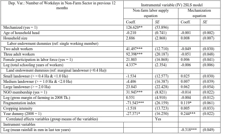
Table 6 IV Model estimates of Labor Supply of Farm Households ...42
Table 7 Endogenous Treatment Effects Model ...44
Table 8 Time Series Properties of the Prices ...72
Table 9 Summary Statistics of the Prices Returns (in Percent) ...73
Table 10 Spearman and Pearson’s Correlation Coefficients for the Prices Changes ...74
Table 11 GARCH (1,1) Results ...77
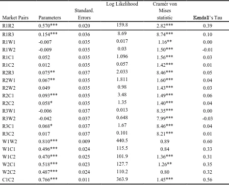
Table 12 Parameter Estimates and Kendall’s Tau of Gaussian Copula ...81
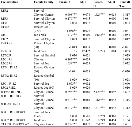
Table 13 Parameter Estimates, Kendall’s Tau and Tail Dependence Estimates of Selected Copula Family ...83
Table 14 C-Vine Copula Model Parameter Estimates ...85
Table 15 D-Vine Copula Model Parameter Estimates ...86
Table 16 Parameter Estimates, Kendall’s Tau and Tail Dependence Estimates of Selected Copula Family ...88
Table 17 Parameter Estimates, Kendall’s Tau and Tail Dependence Estimates of Selected Copula Family ...90
Table 18 Co-Movements of Extreme Price Changes ...92
Table 19 List of Sample Countries ...109
Table 20 Summary Statistics ...111
Table 21 Panel Unit Root Test – Im, Pesaran and Shin (IPS) ...112
Table 22 Hausman Test: Fixed vs. Random ...113
Table 23 Fixed Effects Panel Regression Results (Total Trade) ...115
Table 24 Fixed Effects Panel Regression Results (Disaggregated) ...117
Table 25 Fixed Effects Panel Regression Results with Historical Volatility (Total Trade) ..119
Table 26 Fixed Effects Panel Regression Results with Historical Volatility (Disaggregated) ...120
Table A1 Linear Probability Model (LPM) and Probit Model (including CRE Variables) 126 Table A2 Bivariate probit marginal effects estimates (including CRE Variables) ...127
Table A3 Endogenous Switching Probit Estimates (including CRE Variables) ...128
Table A4 Linear Regression Model of Labor Supply (including CRE Variables) ...129
Table A5 Endogenous Treatment Effects Model (Including CRE Variables) … ...…130
Table A5 Endogenous Treatment Effects Model (Robustness Check excluding top 10%) 131 Table C1 Hausman Test: Fixed vs. Random (Quarterly Data) ...140
Table C2 Fixed Effects Panel Regression Results (Quarterly data) ...140
LIST OF FIGURES
Figure 1 Households' transition to and from the use of labor-saving agricultural technology
between 2000 and 2008 ...26
Figure 2 Scatterplots of Gumbel and Gaussian copula (simulated data, tau=0.5, N=500) ....68
Figure 3 Contour plots of different copulas ...69
Figure 4 Food grain prices (USD/Ton).………...….………...74
Figure 5 Food grain prices (log prices) ...75
Figure 6 Returns of food grain prices (change in log prices) ...75
Figure 7 Scatterplot matrix and correlation among log price changes ...76
Figure 8 Scatterplot matrix and correlations among standardized residuals ...78
Figure 9 Scatterplots and correlations when residuals were transformed into uniform CDF ...79
Figure 10 Scatter and tau for current rice price and lagged price changes for other crops ...89
Figure 11 Scatter and tau for lagged rice price and current price changes for other crops....91
Figure B1 C-vine tree plots among the market pairs ...132
Figure B2 D-vine tree plots among the market pairs ...133
Figure B3 Observed and simulated data are plotted (using bivariate copulas) ...134
Figure B4 Original uniform CDFs data ...138
Figure B5 Simulated data from C-Vine copulas ...138
CHAPTER 1: AGRICULTURAL MECHANIZATION AND NON-FARM LABOR SUPPLY OF FARM HOUSEHOLDS
1.1. Introduction
Economic opportunities in the non-farm sector have long been recognized as an integral
part of rural livelihoods in developing countries (see Lanjouw & Lanjouw, 2001; Lanjouw &
Feder, 2001). The non-farm sector is an important source of employment in many countries,
and it has been a key driver of overall economic development in many East Asian economies
(Lin & Yao, 1999; Lanjouw & Lanjouw, 2001; McCulloch, Timmer, & Weisbrod, 2007). It is
also evident that non-farm income is critical to the welfare of rural households in developing
countries (Rosenzweig, 1988). In many developing countries, a considerable portion of farm
households earn income from non-farm sources, and income from the non-farm sources
constitutes between 20% and 70% of total household earnings (Adams, 2002; Newman &
Gertler, 1994; Reardon, Taylor, Stamoulis, Lanjouw, & Balisacan, 2000; Rizov, Mathijs, &
Swinnen, 2000). One need not be a skilled worker to engage in non-farm economic activities;1
unskilled labor is the primary source of non-farm earnings for the poorest subsistent African
farmers, who often earn a significant share of their income from non-farm sources (Barrett,
Reardon, & Webb, 2001; Reardon, 1997).
The importance of the non-farm sector as a source of rural employment, and as a driver
of rural economic growth and poverty reduction, is growing all over the developing world. For
example, in Bangladesh, growth in rural non-farm income accounted for 40% of poverty
reduction between 2000 and 2005, while growth in farm income contributed only about 21%
in the same period (World Bank, 2013). In Bangladesh, the rural non-farm sector is no longer viewed as “residual” sector, and it remains a persistent employment source of half of the rural
workforce since the mid-1980s (Sen, 1996; World Bank, 2016). The extremely narrow scope
for expanding agricultural land, the growing educated labor force, and the increasing demand
for non-farm goods and services all imply that future economic development policies in
densely populated developing countries will focus on ensuring robust growth of the rural
non-farm sector.
Despite the structural changes in most developing economies, the labor force has not
moved out of agriculture as rapidly as expected, although successful movement of surplus
labor from agriculture to the advanced sector has long been considered to be an important
feature of economic development. Labor migration from the rural farm sector to the advanced
urban sector has been analyzed for many countries and at many points of time (see Lewis,
1954; Harris & Todaro, 1970). However, extraordinary agricultural growth following the “green revolution” and the development of physical infrastructure (e.g. roads, highways, and
bridges) and communication technology (e.g. cell phones, the Internet, etc. ) have expanded
the non-farm sector significantly beyond urban areas. The clear demarcation between the urban
advanced sector and the rural farm economy is disappearing fast in many developing countries.
Thus, farm household members can work both in the farm sector and the non-farm sector
simultaneously; working in the non-farm sector no longer requires the farm household to move
its working members to urban areas, either permanently or temporarily. A farm household may
either part-time or full-time. As an agricultural economy experiences significant shocks and
readjustment, the relocation patterns of a farm household’s labor endowment are critical
characteristics of the rural labor market development, and this issue has drawn attention from
many economists (see Sumner, 1982; Huffman, 1991).
Much theoretical and empirical literature has investigated how a farm household may
allocate its labor hours between farm and off-farm uses through optimization behavior
(Sumner, 1982; Huffman, 1991; Mishra & Goodwin, 1997; and Goodwin & Holt, 2002). Much
earlier literature on the off-farm labor supply of farm households has, however, focused on
modeling and examining the off-farm labor supply effects on farming efficiency and farm
income volatility. A similar question involves the extent to which the off-farm labor supply of
farm households may change in response to agricultural mechanization, or the adoption of
labor-saving technology. Despite its importance to the development process, the economic
literature has not devoted sufficient attention to the joint analysis of farm households’ decisions
about labor supply to the non-farm sector in relation to the technology adoption decision.
The poverty outcomes and agricultural productivity outcomes of agricultural
modernization have been studied extensively in the literature on agricultural mechanization
(see David & Otsuka, 1994; deJanvry & Sedoulet, 2002; Evenson & Gollin, 2003; Minten &
Barrett, 2008). Despite some earlier studies focused on the effects of agricultural
mechanization on employment and wage earnings of poor and tenant farmers (Binswanger &
Braun, 1991; The Nuffield Foundation, 1999; Minten & Barrett, 2008), the general labor
market responses of farm households to agricultural mechanization have been overlooked.
soybeans by farm households has positive effects on off-farm income. However, the
herbicide-tolerant soybeans are not a labor-saving technology in the strict sense; they simply reduce
management time. Ahituv and Kimhi (2002) find that farm capital investment reduces the farm households’ participation in the off-farm employment opportunities, implying that family labor
and farm capital are complements in agricultural production.
Over the last few decades, agriculture in most developing countries has undergone a
significant structural transformation. Developing nations (except the nations in sub-Saharan
Africa), have adopted labor-saving agricultural technologies at an unprecedented level.
Intensification of production systems has created power bottlenecks around \ land preparation,
harvesting, and threshing operations, even in the densely populated Asian countries; these
power bottlenecks are alleviated with the adoption of labor-saving agricultural technology,
which in turn raises agricultural productivity and reduces the per-unit cost of crop production
(Pingali 2007). Tractors number in India rose from 0.19 per 1000 hectares in 1961 to 9 per
1000 hectares by 2000 (Pingali, 2007). Mandal (2002) estimates that, in Bangladesh, around
150,000 power tillers have been imported annually since liberalized import policies were
implemented in the mid-1990s.
Mechanization has often been considered by the critics as detrimental for densely populated “labor surplus” countries, because of the negative effects of mechanization on
agricultural employment in terms of displacement of labor and tenant farmers. If that argument
is true, then what are the rationales of rapid mechanization of power-intensive operations even
in Asian countries with high population densities and low wages, such as India, Bangladesh
instead that the mechanization of power-intensive operations (water lifting, tillage, milling,
etc.) have minimal labor displacement effects (Pingali 2007). Hormozi, Asoodar, & Abdeshahi
(2012) find a strong positive correlation between agricultural mechanization and the technical
efficiency of rice producers in Iran. The productivity effects of agricultural mechanization can
come from three sources: yield changes, area expansion, and labor savings. The evidence
presented in the literature indicates that, for power-intensive operations, generally no significant yield difference exists between animal draft and tractor tillage (Herdt, 1983;
Binswanger, 1978). If we find no yield differences between animal draft and tractor farms, we
must conclude that the transition to tractor-drawn plows is rarely motivated by improvement
in tillage quality. Area expansion and/or labor saving must be the driving forces for such a
transition. In densely populated countries, the ability to expand the area under cultivation is
extremely narrow, which is clearly indicated by the tiny amount of arable land per agricultural
worker (for example, 0.26 hectare per worker over 2006–2011 in Bangladesh, according to the
Food and Agriculture Organization [FAO]).
The evidence presented in the literature indicates that, for power-intensive operations, the productivity benefits of mechanization consist mainly of labor savings. Pingali, Bigot, and
Binswanger (1987) reviewed 24 studies on labor use of farm households, and 22 of the 24
studies reviewed reported lower total labor use per hectare of crop production for tractor farms
compared to draft animal farms. Twelve studies reported reductions in labor use of 50% or
more. The greatest reduction in labor use was for land preparation, which was reduced by 50%
through agricultural mechanization been put? The answer to this issue has been hypothesized
in the relevant literature to be non-farm use.
Excellent non-farm employment opportunities may induce farm households—even
those in densely populated countries with land scarcity—to mechanize farm operations.
Cultivators became prevalent in Japan during the late 1950s, when agricultural wages rose
sharply in response to high labor demand from post-war industrialization (Ohkawa, Shinohara,
& Umemura, 1965). In recent decades, fast-growing south Asian countries like Bangladesh
and India have shown a similar trend, experiencing significant rural labor market tightening
with a pronounced increase in rural real wages (Hnatkovska & Lahiri, 2013; Hossain, Sen, &
Sawada, 2013). The use of labor-saving technology (e.g. tractors, threshers, etc.) in agriculture,
and the rapid expansion of the non-farm sector have enabled farm households to reallocate
their underemployed agricultural labor time toward more highly productive off-farm work in
the non-farm sector.
This chapter examines whether agricultural mechanization could induce farm
households to participate in, and to supply more labor hours in, the non-farm sector. Existing
literature about farm households holding multiple jobs has mainly studied the United States
and other developed countries (see Goodwin & Holt, 2002; Goodwin & Mishra, 2004).
Research on farmers in low-income countries holding multiple jobs is scarce. Moreover, there has been little research into how farm households’ adoption of labor-saving technology affects
the off-farm labor supply. This chapter uses a unique longitudinal survey data set from rural
Bangladesh to investigate the role of the labor-saving technology adoption in farm production
is used to establish the relationship between labor-saving technology adoption and the off-farm
labor supply decisions of farm households through the elasticity of substitution between labor
and capital in agricultural production.
The increase of market-based rentals of agricultural technology in Bangladesh brings
the benefit of modern technology within the reach of subsistence farm households. For
example, about 89% of farm households use tractor or power tillage for land preparation in
agricultural production, while only 5% farm households own a tractor/power tiller. This
structural shift has changed the input ratios used in farm production. A tractor/power tiller is
regarded as labor-saving technology, and the use of tractor/power tillage reduces the labor
requirement in land preparation, thus releasing extra labor hours. Thus, the joint analysis of
agricultural households’ decisions regarding the adoption of labor-saving technology and their
off-farm labor supply will add additional knowledge to the relevant literature. The adoption of
mechanized technology raises agricultural productivity, which in turn increases returns to time
employed in farming. Thus, an income effect could increase the farm operator’s leisure time,
while a substitution effect could raise the amount of time used in farm production. Because
most farming in developing countries is subsistence farming, and because of extremely low
arable land per capita, the ability for most farm households to raise work hours in the farm
sector is somewhat limited. Thus, the farm operator may instead supply labor hours in the
non-farm sector as long as returns from the non-non-farm sector are higher than the opportunity cost of
leisure time. Through this dynamic, the adoption of mechanized technology in farming could
The population density in Bangladesh is the highest in the world, and the challenge to
agricultural livelihoods is clearly indicated by the tiny amount of arable land per agricultural
worker (0.26 hectare per worker over 2006–11, according to FAO). Certainly, rural farm
households need to diversify their income sources and livelihood strategies, both to manage
risks and to ensure more rapid income growth. The evidence suggests that such diversification
is well underway in Bangladesh (Sen, 2003; World Bank, 2016). While absolutely and
functionally landless households depend on the rural non-farm economy for their survival,
farm households are also increasingly engaging in non-farm economic activities, both to
diversify the risks of farm income volatility from price shocks and production loss, and to
smooth consumption in the lean season.
The main objective of this study is to explore the impact of agricultural mechanization
on the labor supply behavior of farm households. Specifically, it examines the off-farm
participation effects of the adoption of labor-saving farm technology. This chapter looks at the
joint decisions of off-farm labor supply and the labor-saving technology adoption of farm
households using primary data obtained from a nationally representative longitudinal survey
data for the years of 2000 and 2008.2
The rest of the chapter is organized as follows. Following the introductory discussions
in Section 1.1, Section 1.2 outlines the conceptual and theoretical framework. Section 1.3
describes the econometric model employed for estimation; Section 1.4 presents and discusses
data sources, sampling strategy, and summary results; and Section 1.5 presents the results of
econometric models and the analysis of the results. The chapter ends with concluding remarks
and policy implications in section 1.6.
1.2. Theoretical Model
The chapter uses the agricultural household model, developed by Singh, Squire, and
Strauss (1986) and modified by Sadoulet and deJanvry (1995), to establish the relationship
between the labor-saving technology adoption decision and the off-farm labor supply decision
through the elasticity of substitution between labor and capital in farm production. Goodwin
and Holt (2002) and Farnandez-Cornejo et al. (2005) modified this agricultural household
model to study the off-farm labor supply decisions of farm households in Bulgaria and the
United States, respectively. We use the Goodwin and Holt (2002) and Farnandez-Cornejo et
al. (2005) version of the agricultural household model, introducing the agricultural technology
adoption decision into the production techniques, to identify the off-farm labor supply function
of farm households. The significant difference between this study and the earlier works of
Goodwin and Holt (2002) and Farnandez-Cornejo et al. (2005) is that we treat the farm
household as an economic agent instead of a farm operator. This is because the independence
among individuals within the same household could not be assumed; household members’
economic decisions are jointly determined. The labor supply decisions of rural farm
households in developing countries are governed by the household’s utility maximization
problem, which is subject to constraints on total time endowment, income, and farm production
technology. Households’ members are assumed to receive utility from a vector of members’
leisure and non-economic activities at home (l), a vector of purchased goods (q), and a vector
exogenous to the household’s decisions. Farm households maximize utility (U) subject to
income, technology, and time constraints. The agricultural household utility function can be
modeled as
𝑈 = 𝑈(𝑞, 𝑙; 𝑧) (1.1)
where U is assumed to have the usual regularity properties of a utility function, such as
twice differentiability, quasi-concavity, and increasing in 𝑞, 𝑙, and z. Farm households generate
utility from consumption of good 𝑞; from leisure 𝑙, which also includes home time; and from
other household characteristics 𝑧, such as human capital, age, household size, and so on. The
model assumes that marginal utility of consumption good and leisure approaches infinity as
consumption goes to zero, which ensures that a positive amount of consumption good and
leisure are always consumed.
The objective of the farm household is to maximize utility from the consumption of
goods and leisure subject to the farm production, income, and time constraint. The income,
farm production technology, and time constraints can be represented as
𝑝𝑐𝑞 + 𝑟𝑋(𝑇) = 𝑝𝑓𝑄 + 𝑤𝑀 {Income constraint} (1.2)
𝑄 = 𝑄{𝑋 (𝑇), 𝐹(𝑇), 𝐷)} {Technology constraint} (1.3)
𝐻 = 𝑀 + 𝐹(𝑇) + 𝑙 {Time constraint} (1.4)
in X. M denotes the labor time spent in off-farm work. Unlike Goodwin and Holt (2002) and
Farnandez-Cornejo et al. (2005), we exclude income from other sources (e.g. capital gains,
interest income, etc.) in our income constraint, as income from other sources is rare among
Bangladeshi farm households. Farm income depends on the price of agricultural output, 𝑝𝑓; on input prices, r; and on the amount of time spent on farm works, F.
Equation (1.3) represents a household’s technology constraint, where F is labor time
devoted to the farm and 𝑇 stands for the farm household’s labor-saving technology adoption
decision. The adoption of labor-saving technology reduces the labor requirement in farm
production. Thus, the adoption of agricultural technology should be incorporated into the
production technology implicitly, not as a shifter of the production function. D is a vector of
exogenous factors that shift Q. The production technology is assumed to have all the regularity
conditions, such as twice differentiable, increasing in inputs, etc.
Equation (1.4) is the time constraint of the agricultural household. Each household has
a fixed amount of time, H, which is allocated among farm work, off-farm work, and leisure.
This agricultural household model assumes that marginal productivity of farm labor
approaches to infinity while on-farm work is zero, implying interior solution of the model, 𝐹 >
0. However, off-farm labor works, M, could be zero as well, 𝑀 ≥ 0.
Plugging (1.3) into (1.2), we combine the technology and the income constraint into
the following constraint:
Now we can solve the agricultural household model, given the differentiable utility
function and given 𝜆 𝑎𝑛𝑑 𝜇 as the Lagrange multipliers of the income and the time constraints,
respectively:
𝐿 = 𝑈(𝑞, 𝑙, 𝑑) + 𝜆[𝑝𝑓𝑄(𝑋(𝑇), 𝐹(𝑇), 𝐷) + 𝑤𝑀 + 𝐴 − 𝑝𝑞 − 𝑟𝑋(𝑇)] + 𝜇[𝐻 − 𝑀 −
𝐹(𝑇) − 𝑙].
The Kuhn-Tucker first-order conditions are:
𝜕𝐿
𝜕𝑞 = 𝑈𝑞− 𝜆𝑝 = 0 (1.6)
𝜕𝐿
𝜕𝑙 = 𝑈𝑙− 𝜇 = 0, (1.7)
𝜕𝐿 𝜕𝑇 = 𝜆 [𝑝𝑓 {( 𝜕𝑄 𝜕𝑋) ∗ ( 𝜕𝑋 𝜕𝑇) + ( 𝜕𝑄 𝜕𝐹) ∗ ( 𝜕𝐹 𝜕𝑇)}] − 𝑟 ( 𝜕𝑋 𝜕𝑇) − 𝜇 ( 𝜕𝐹
𝜕𝑇 ) = 0 (1.8)
𝜕𝐿
𝜕𝑋 = 𝜆[ 𝑝𝑓 𝜕𝑄
𝜕𝑋 – 𝑟] = 0 (1.9)
𝜕𝐿
𝜕𝐹 = 𝜆 𝑝𝑓 𝜕𝑄
𝜕𝐹 – 𝜇 = 0 (1.10)
𝜕𝐿
𝜕𝑀 = 𝜆𝑤 − 𝜇 ≤ 0, 𝑀 (𝜆𝑤 − 𝜇) = 0 (1.11)
𝜕𝐿
𝜕𝜆 = 𝑝𝑓𝑄(𝑋(𝑇), 𝐹(𝑇), 𝐷) − 𝑤𝑀 + 𝐴 − 𝑝𝑞 − 𝑟𝑋 = 0 (1.12)
𝜕𝐿
Given the positive amount of labor supply to off-farm work, an interior solution occurs
and equation (1.10) and (1.11) hold with equalities. From equation (1.10) and (1.11), we can
reach a familiar condition:
𝑝𝑓 𝜕𝑄
𝜕𝐹 = 𝑤 (1.14)
The marginal value of the farm labor must be equal to the off-farm wage rate. Solving
equations (1.6), (1.7), and (1.11) would give us another familiar condition:
𝑈𝑞
𝑈𝑙 =
𝑝
𝑤 (1.15)
The condition in (1.15) implies that the marginal rate of substitution between
consumption and leisure should be equal to the ratio between the price of consumption good
and the wage rate.
When an interior solution occurs, equations (1.9) and (1.10) can be solved
independently to obtain farm labor demand as optimal consumption, and production decisions can be separated because the value of the household’s time is determined by the off-farm wage
rate: ( 𝑤 = 𝜇
𝜆 ) (Huffman, 1991).
Solving the model, we could find following on-farm labor demand functions and input
demand functions:
F* = F( r, w, 𝑝𝑓,T, D) (1.16)
Substituting these optimal input demand functions into the technology constraint (1.3)
would give us optimal output, as follows:
Q* = Q( r, w, 𝑝𝑓, T, D) (1.18)
Solving jointly equations (1.6), (1.7), (1.12), and (1.18), a household’s optimal amount
of leisure demand and consumption good can be derived as follows:
𝑙 * = 𝑙 ( r, w, 𝑝𝑐, 𝑝𝑓, 𝑇, 𝐷) (1.19)
q* = q( r, w, 𝑝𝑐,𝑝𝑓, 𝑇, 𝐷) (1.20)
Plugging optimal leisure hours and on-farm labor demand into the time constraint, the
derived supply of off-farm labor (Huffman, 1991) is as follows:
𝑀∗ = 𝐻 − 𝐹∗− 𝑙∗
= M( r, w, 𝑝,𝑝𝑓, 𝑇, 𝐷, 𝑧) (1.21)
Equation (1.21) implies that, given a constant total amount of labor endowment of a
farm household, the adoption of labor-saving technology in agricultural production would
result in a higher level of labor supply to the non-farm sector.
1.3. Econometric Methodology
The goal of this chapter is the estimation of the off-farm labor supply decisions of farm
household.3 Therefore, we follow a simple reduced-form model of off-farm labor supply to
estimate the effects of agricultural mechanization on the off-farm labor supply decisions. The
theoretical framework for the model of off-farm labor supply decisions suggests that all
observable farm household characteristics that affect wages, prices, production, and utility
should be included in the estimation of off-farm labor supply decisions.
To estimate the non-farm participation effects of the adoption of labor-saving
agricultural technology, we use following regression specification based on the theoretical
background given in the preceding section:
𝑃𝑖𝑡 = 𝛼 + 𝛽𝑋𝑖𝑡 + 𝛿𝑍𝑖𝑡 + 𝜌𝑡+ 𝜀𝑖𝑡 (1.22)
𝑃𝑖𝑡 denotes the participation/labor supply of ith household in the rural non-farm (RNF) sector at year t. 𝑋𝑖𝑡 is a vector that includes number of variables representing households’ and workers’ characteristics. 𝑍𝑖𝑡 attributes a household’s agricultural technology adoption status.
Year-specific effects are represented by 𝜌𝑡, while 𝜀𝑖𝑡 stands for idiosyncratic normally distributed error terms.
Two separate versions of the model (1.22) need to be used to estimate the effects of the
adoption of labor-saving technology adoption by farm households on their off-farm labor
supply decisions. The first version models the participation decision and the second set models
the magnitude of labor supply to the off-farm work. An ordinary least square (OLS) estimation
of linear probability model (LPM) or the maximum likelihood estimation of probit of equation
(1.22) can estimate the impact of the technology adoption on the non-farm participation
decision. Similarly, an OLS, or the maximum likelihood estimation of endogenous treatment
effects (ETE) of equation (1.22), can estimate the impact of technology adoption on the extent
of non-farm labor supply. The participation decision model of equation (1.22) can be presented
as follows:
𝑃𝑖𝑡∗ = 𝛼 + 𝛽𝑋𝑖𝑡+ 𝛿𝑍𝑖𝑡+ 𝜌𝑡+ 𝜀𝑖𝑡 (1.23)
Where 𝑃𝑖𝑡∗ ≥ 0 if 𝑃𝑖𝑡 = 1
𝑃𝑖𝑡∗ < 0 if 𝑃𝑖𝑡 = 0
Where 𝑃𝑖𝑡stands for the non-farm participation (NFP) decision (probit). 𝑃𝑖𝑡∗ is a latent
variable that is unobserved if 𝑃𝑖𝑡∗<0.
The labor supply decision model of equation (1.22) can be presented as follows:
𝑃𝑖𝑡 = 𝛼 + 𝛽𝑋𝑖𝑡+ 𝛿𝑍𝑖𝑡+ 𝜌𝑡+ 𝜀𝑖𝑡 (1.24)
Here, 𝑃𝑖𝑡stands for the labor supply decision.
Estimating the impact of technology adoption on the participation and the labor supply
behavior of farm households, however, presents some difficulties. When the unobserved households’ characteristics (e.g. skill and abilities of workers) are correlated with both the
off-farm work decision and the technology adoption decision, spurious correlations might be
produced, which might give biased estimates of the effects of technology adoption on the
non-farm sector can adopt labor-saving technology to substitute the foregone labor hours that
are supplied to the non-farm sector. Thus, the OLS regression of the off-farm work decision
on the technology adoption decision might be capturing the positive "effect" of reverse
causality. Though the workers’ schooling may capture their capacity and skill to some extent,
it is, in general, not possible to control for all such potential confounding factors in a regression
specification, and thus regression results that do not account for endogeneity may be
misleading. To control for the possible endogeneity between the technology adoption decision
and the off-farm labor supply decision, an instrumental variable (IV) approach is used to
estimate the relevant models of equation (1.23) and (1.24).
For the participation equation, the study follows three standard econometric methods:
the instrumental variable (IV) approach, the bivariate probit model (BPM), and the endogenous
switching probit model (SPM). While the IV approach with a binary dependent variable may
encounter the limitations of a linear probability model (LPM), the IV version of the LPM model
facilitates several tests that examine the validity of the relevant instruments, and we expect that
the validity tests of instruments will be untroubled by the limitations of LPM in the IV model.
However, the main results regarding the non-farm participation effects of labor-saving
technology adoption are drawn from the BPM and the SPM, which are particularly designed
for dealing with a binary dependent variable with endogenous dummy treatment variables.
Both the BPM and the SPM rely on normality assumptions. The SPM, however, is more
efficient, as it relaxes the participation equation’s assumption of equality of coefficients in two
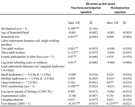
regimes. We have estimated both models for two reasons. First, the BPM provides average
marginal effects (hereafter, AME) of all the covariates in the participation equation, as well as
effects for all the covariates is a cumbersome process in the SPM. Second, the SPM provides
regime-specific coefficients for all the covariates, which offers insight into the regime-specific
role of covariates; in contrast, the BPM assumes equality of coefficients in the participation
equation across the regimes. Moreover, estimating both models helps us to check the
robustness of the estimates of ATE.
For the same reasons, we also follow the two standard econometric approaches (the IV
approach and the ETE model) with the labor supply equation. Although the use of a linear IV
model with an endogenous dummy regressor is inefficient, we use this model to check the
validity of instruments. Given the binary nature of the endogenous regressor that represents
the labor-saving technology adoption decision, the ETE model is the most efficient one for
estimating the labor supply effects of the technology adoption in farm production. The ETE
model also allows censoring the sample for which the non-farm labor supply is not observed.
Given the longitudinal nature of the data set used for this chapter, the use of the
fixed-effects model would be ideal. But the fixed-fixed-effects model suffers the “incidental parameter problem” and excludes the variables that do not vary over time. However, Mundlak (1978) has
shown that, for balanced panel data, the fixed-effect estimator can be generated from pooled
OLS estimators by adding the time means of the covariates as additional explanatory
covariates. Wooldridge (2013) extends the work of Mundlak (1978) to unbalanced panel data
and nonlinear panel data models. Thus, we follow correlated random effects (CRE) estimation
for each specification to avoid the incidental parameter problem and to get the fixed-effects
1.3.1. Identification Strategy
The initial challenge to establishing the causal impact of the technology adoption
decision on non-farm participation decisions is the possibility of unobserved characteristics of
farm households that simultaneously affect their non-farm participation decisions and their
technology adoption decisions. For example, farm households with educated working
members may participate in the non-farm sector to diversify their earning sources, and may
adopt modern agricultural production technology to substitute their foregone labor hours. A
simple comparison between the percentages of non-farm participation among the
technology-adopting farm households and the non-technology-adopting farm households would overstate the non-farm
participation effects of the adoption of labor-saving technology. Alternatively, small or
marginal farm holdings, which may not be appropriate for the use of labor-saving technology,
may forego participation in the rural non-farm sector because of labor constraints, which might
lead to a spurious negative relationship between farm households’ non-farm participation
decision and technology adoption decision. Therefore, the direction of selectivity bias is
theoretically uncertain.
We therefore follow the IV approach to reduce selectivity bias. We use village-level
average rainfall in the previous 10 years, the presence of operating land with clay loam soil,
and operating land with a very high level of elevation as instruments for the likelihood of a household’s adoption of tractor or power tiller for land preparation in farm production. Higher
rainfall makes the tillage process easier, inducing farm operators to rely less on mechanized
tillage and more on family labor and cattle/bullocks for land preparation. Heavy rainfall also
loam soil is difficult to till, thus inducing farm operators to use mechanized tillage. A
household with clay loam soil is 3% more likely to use mechanized tilling than a household
without clay loam soil. Land with high elevation is close to homestead land and thus induces
households not to use hired mechanized tillage, and to instead use family labor and
cattle/bullocks for tilling. Farm households that operate land with high elevation are less likely
to adopt mechanized tillage. Thus, the use of rainfall, soil quality, and land elevation are valid instruments for a household’s mechanization decision.
Our identification strategy is that all these instruments, apart from their influence on
the households’ tractor/power tiller use, do not affect the non-farm participation decision of a
farm household. Instrumental variable estimation relies on this exogeneity assumption. Thus,
the validity of the instruments is crucial for reliable estimates. One potential threat is that
rainfall in a village might influence farm productivity, which in turn affects the non-farm
participation decision, which in turn affects the technology adoption decision. Considering this
possibility, we control for the farm productivity by incorporating gross margin in farm
production of each farm household. The validity of the instruments has been checked as well,
and the instruments have passed all the relevant tests for weak identification and
overidentification.
1.4. Data and Summary Statistics
The data for this study are drawn from a unique longitudinal survey of a nationally
representative sample of rural households in Bangladesh. The survey spanned about two
by the Bangladesh Institute of Development Studies (BIDS) in 1988.4 It included 1,240 rural
households from 62 villages in 57 out of 64 districts in Bangladesh and studied the impact of
technological progress on income distribution and poverty in Bangladesh (Hossain, Quasem,
Jabbar, & Akash, 1994; Rahman & Hossain 1995). The households were revisited in 2000,
2004, and 2008. However, we could access only data for 2000 and 2008; therefore, this study
limits its analysis to the 2000 and 2008 data. The sample size in the repeat surveys of 2000 and
2008 were 1880 and 2010, respectively. The information was collected through a
semistructured questionnaire designed to gather information on demographic details, land use,
costs of cultivation, livelihoods, farm and non-farm activities, commodity prices, ownership
of non-land assets, income, expenditure, and employment. In addition to these data, the dataset provides extensive details of the farms’ characteristics, including details on soil type, elevation,
irrigation sources, and tenurial arrangements, among others.
To study the off-farm labor supply effects of agricultural technology adoption using a
panel survey, the problem of the splitting of households needed to be addressed, as household-splitting makes it difficult to compare the households’ performances over time. Splitting of
households is a very common scenario in rural Bangladesh, especially after the death of the
household head, typically the father. Thus, the splitting of the household has serious
implications for land and other non-land asset endowments. Among the original 1880 sample
households that were surveyed in 2000, 1598 households (about 85%) remained intact
4 The benchmark survey used a multistage random sampling method. The sample size has been adjusted in each round of
throughout the period of 2000–2008. Thus, household splitting and attrition from migration
occurred at a rate of nearly 1.9% per year for the period of 2000–08. Among the 1598 intact
households, we use 852 sample households in our analysis; the rest of the households were not
involved in farm production in either 2000 or 2008.5
The main advantage of the 62-village panel survey over repeated cross sections (such
as Household Income and Expenditure Survey (HIES) or Labor Force Survey (LFS)) is the
ability to track the employment status of the same household over time. Looking at the multiple
cross-section surveys (for example, HIES and LFS), there is little movement of rural labor
forces between the farm sector and the non-farm sector. Between 2000 and 2010, according to
the Bangladesh Bureau of Statistics (BBS), the share of the RNF sector in total rural
employment has increased by only 1%, from 44.5% in 2000 to 45.5% in 2010 (BBS, 2013).
This number, which is based on the repeated cross-section surveys, shows that the net
movement of the rural workforce between farm and non-farm activities often fails to capture
the ultimate employment dynamics in rural Bangladesh. Analysis of labor supply decisions of
farm households based on longitudinal data is thus not just about capturing employment trends;
it enables us to look beyond mere statistical aggregates and shed light on causalities of
long-term employment patterns. The panel waves capture the decisions of the same households over
time. This leads to better understanding of the possible policy support necessary to further
support the movement of the rural workforce toward better non-farm opportunities.
5The inclusion of the ‘‘split households’’ creates difficulties in estimating changes in the asset base of the household, an
The panel nature of the data allows us to identify several dynamic-employment groups
on the basis of their diverse movements in and out of the non-farm sector. For the purpose of
analyzing employment dynamics, we have generated two groups of households based on their
work status. Sample farm households that remain exclusively in farming (all the working
members of a household are involved in agricultural activities only) are categorized as “farm only,” while the farm households that also engage in non-farm activities (any of the working
members of the household are involved in any kind of non-farm activities)6 are considered as
“non-farm participants.” Patterns of participation in the non-farm sector and transformation
over time are presented in Table 1.
Table 1 reveals a strong mobility between the farm sector and the non-farm sector
throughout the period of 2000–2008. A significant portion of sample households moved back
and forth between the farm-only status and the non-farm participant status; from 2000 to 2008,
there were 338 households (39.7% of the total sample of 852 households) that retained
farm-only status, while 212 households (24.9% of the total sample) remained non-farm participants
(Table 1). The other two categories indicate the changing employment patterns: one group
initiated participation in non-farm activities, while the other pulled themselves out of non-farm
activities and returned to farm-only status. In the same period, 133 households (15.6% of 852
households) initiated participation in non-farm economic activities and 169 households (19.8%
of the total sample) moved out of non-farm activities.
6Farm activities include farming, fishing, poultry and livestock rearing, forestry, and agricultural wage labor. Non-farm
Two immediate observations follow from the above discussion. First, gross movements
of the rural workforce between farm and non-farm activities are much larger than the net
changes in the sectoral employment trends over time reveal. Second, it is important to study
the drivers of change underlying the movements of rural households between farm and
farm activities to understand better the causes of movements of rural workforce toward
non-farm economic opportunities. Studying these movements provides deeper insights into the
mechanisms that boost the participation of rural households in the non-farm sector than merely
studying the characteristics of the non-farm participants over time, and may provide avenues
for attacking the underemployment of family labor in farm production in developing countries.
Table 1: Transition Between Work Statuses
Work status in 2008 Worked only
on-farm
Worked
off-farm Total
Work status in 2000
Worked only on-farm N 338 133 471
Percent 39.67 15.61 55.28
Worked off-farm N 169 212 381
Percent 19.84 24.88 44.72
Total N 507 345 852
Percent 59.51 40.49 100
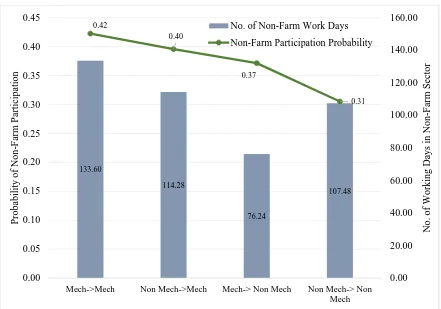
Table 1 relates the labor-saving technology adoption decision to the non-farm
participation decision of farm households. The probability of participating in the rural
non-farm sector is the highest (0.42) for households that remained users of agricultural technology
throughout the period between 2000 and 2008; the probability is lowest (0.31) for households
of farm participation is also higher for households that changed their status from
non-adopters of agricultural technology in 2000 to users in 2008 than in households that remained
non-users in 2008. The bar chart also shows that households that adopt labor-saving
agricultural technology work more in the non-farm sector than do households that do not adopt
the labor-saving agricultural technology. Farm households that remained users of agricultural
technology between 2000 and 2008 worked, on average, 133 days in the rural non-farm sector; households that didn’t adopt the labor-saving land-preparation technology in the same period
worked, on average, 107 days in the rural non-farm sector. Households that moved from being
non-users of agricultural technology for land preparation to being users of this technology
between 2000 and 2008 worked, on average, 114 days in the rural non-farm sector. On the
other hand, households that were technology users in 2000 and were not technology users in
Figure 1. Households' transition to and from the use of labor-saving agricultural technology between 2000 and 2008.
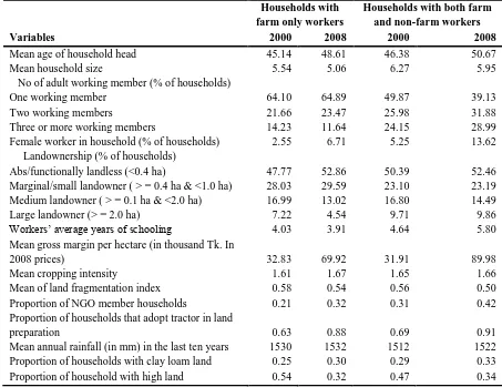
Summary statistics of the key variables are provided in Table 2. As Table 2 shows, the
mean age of household head increases over time regardless of the sector of employment.
Households with more working members, higher family size, and greater female labor force
participation are more inclined to participate in the rural non-farm sector. These statistics imply
that households with more working members are more likely to diversify their employment
out of agriculture. As expected, schooling helps rural households to move out of farming and
to get into non-farm sector opportunities. For households working only on-farm, the average
number of years of school attended was around four between 2000 and 2008; for households
133.60 114.28 76.24 107.48 0.42 0.40 0.37 0.31 0.00 20.00 40.00 60.00 80.00 100.00 120.00 140.00 160.00 0.00 0.05 0.10 0.15 0.20 0.25 0.30 0.35 0.40 0.45
Mech->Mech Non Mech->Mech Mech-> Non Mech Non Mech-> Non Mech No . o f W o rk in g Day s in No n -Far m Secto r P ro b ab ilit y o f No n -Far m P ar ticip atio n
Households' Trasition in terms Labor-Saving Technology Adoption between 2000 and 2008
that participated in the non-farm sector during the same period, the figure was around five
years of school.
The likelihood of non-farm participation of rural farm households is found to be
sensitive to the initial asset position, e.g. the amount of land owned (Table 2). For the period
from 2000 to 2008, the proportion of households that participated in the non-farm sector
remained almost stagnant for the categories of marginal/small and large landowners; it
declined for the medium landowner category; and it increased for the absolutely/functionally
landless households. The propensity of NGO membership was higher among the non-farm
participant households than the farm-only households; the difference was about 10% between
2000 and 2008. The returns from agricultural land and family labor (proxied by gross margin
of farm production) were slightly lower in 2000 for households with non-farm participation
than the households with farm only status. However, the gross margin of agricultural
production for the non-farm participant households was 30% higher in 2008 thanthat of the
farm-only households. Land fragmentation often is to blame as a source of inefficiency in
farming; high land fragmentation requires more labor time, as it is time-consuming to travel
between plots. Here we find that land fragmentation was higher among the farm households
that remained exclusively in farming in both years.7
Table 2 also presents summary statistics for the instruments used in the estimation. The
rainfall was usually lower for households that participated in the RNF sector. The proportion
7 The land fragmentation index is constructed following the formula of Simpson’s concentration index as follows:
𝑆 = 1 − [∑ ( 𝑎𝑖 ∑ 𝑎𝑖)
2 𝑛
𝑖
]
of farm households with clay loam land was higher among the participant households than
non-participant households. The likelihood of having land with high elevation was greater
among the farm-only households than the non-farm participant households in 2000; this was
reversed in 2008.
The age of the farm household head may represent a general experience that increases
the marginal value of time in each activity, and younger household heads are expected to
participate more in the non-farm sector. The sign of the age variable is thus expected to be
negative. Having more than one working member in the family may have a positive effect on
non-farm labor participation. Larger household size may have either positive or adverse effects
on non-farm labor participation. Female labor force participation is expected to have a positive
effect on non-farm labor participation. Farm operators’ educational qualifications may
positively affect non-farm labor participation. Land ownership may be negatively related to
non-farm labor participation, because having less land may require less labor in farming, which
in turn may induce the farmer to work in the off-farm sector. Both land fragmentation and the
gross margin from farming are expected to have adverse effects on non-farm labor
participation.
The propensity of households to participate in the non-farm sector is also found to be associated with households’ technology adoption, as non-farm participant households are more
likely to adopt the technology. The adoption rates are 63% and 88% among the households
with farm-only status in 2000 and 2008, respectively; among the non-farm participant
Table 2: Descriptive Statistics of the Covariates
Households with farm only workers
Households with both farm and non-farm workers
Variables 2000 2008 2000 2008
Mean age of household head 45.14 48.61 46.38 50.67
Mean household size 5.54 5.06 6.27 5.95
No of adult working member (% of households)
One working member 64.10 64.89 49.87 39.13
Two working members 21.66 23.47 25.98 31.88
Three or more working members 14.23 11.64 24.15 28.99
Female worker in household (% of households) 2.55 6.71 5.25 13.62
Landownership (% of households)
Abs/functionally landless (<0.4 ha) 47.77 52.86 50.39 52.46
Marginal/small landowner ( > = 0.4 ha & <1.0 ha) 28.03 29.59 23.10 23.19
Medium landowner ( > = 0.1 ha & <2.0 ha) 16.99 13.02 16.80 14.49
Large landowner (> = 2.0 ha) 7.22 4.54 9.71 9.86
Workers’ average years of schooling 4.03 3.91 4.64 5.80
Mean gross margin per hectare (in thousand Tk. In
2008 prices) 32.83 69.92 31.91 89.98
Mean cropping intensity 1.61 1.67 1.65 1.66
Mean of land fragmentation index 0.58 0.54 0.56 0.50
Proportion of NGO member households 0.21 0.32 0.31 0.42
Proportion of households that adopt tractor in land
preparation 0.63 0.88 0.69 0.91
Mean annual rainfall (in mm) in the last ten years 1530 1532 1512 1522
Proportion of households with clay loam land 0.25 0.30 0.29 0.33
Proportion of household with high land 0.54 0.32 0.47 0.34
1.5. Results and Discussion
1.5.1. Participation Equation
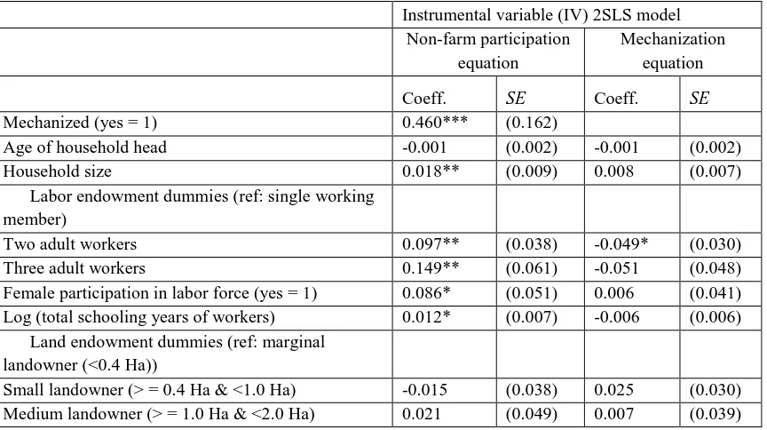
This section presents the results from the estimation of the participation equation. First,
an instrumental variable (IV) model is used, despite its limitation with the use of binary
outcome variables, to examine the validity of the relevant instruments. The estimates from both
the first and second stages of IV, along with many other test statistics, are reported in Table 3.
Durbin’s score statistics and the Wu-Hausman test reject the hypothesis that the technology
adoption decision of a farm household is exogenous to the off-farm participation decision of
that household. For the validity of instruments for an endogenous regressor, instruments must
pass the orthogonality condition (that instruments are orthogonal to the outcome variable). All
three instruments pass Sargan’s orthogonality test, because the test statistics fail to reject the null hypothesis of the instruments’ orthogonality to the non-farm participation decision.
Besides being orthogonal to the outcome variable, instruments also must be correlated with the
endogenous regressor. In likelihood-ratio (LR) IV redundancy tests, the null hypothesis of an instrument’s redundancy has been rejected for each instrument. The instruments pass all the
necessary tests (e.g. underidentification test, weak identification test, and overidentification
test), indicating that they are valid instruments of the endogenous regressor.
Although the explanatory variables from the outcome equation are mostly statistically
insignificant in the first-stage regression of determining the technology adoption decision, all
the instruments are statistically significant. One percent more rainfall reduces the probability
of the technology adoption by 0.3. All the relevant tests (Hausman, Wu-Hausman, and Durbin’s score) confirm the presence of endogeneity between the non-farm participation
decision and the technology adoption decision of farm households. The F-stat at the first-stage
regression also passes the “more than 10” rule of thumb, implying that the excluded
instruments are valid and significantly relevant. We have implemented the Montiel-Pflueger
robust weak instrument test, as the large values of effective F statistics in this test correspond
All instruments pass the test, because the effective F statistic at 5% confidence level
(17.5) is well above the generalized two-stage least square (TSLS) critical value at 5%
worst-case bias (13.42).Thus, the use of rainfall, soil quality, and land elevation as instruments for
the adoption of tractor/power tiller in land preparation does not suffer the usual weak
instrument problems.
The results in the second stage indicate that the adoption of labor-saving tillage systems
raises the probability of non-farm participation by 0.46. Thus, the impact of technology
adoption on the non-farm participation of farm households is quite high. As we are aware of
the limitations of LPM, we should use these results with caution. Although all predicted
probabilities remained within the band of unity, the disturbances were not homoscedastic.
Thus, the coefficients that are presented in Table 2 are unbiased but not consistent. To
overcome this consistency problem, we use a probit model with robust standard errors.
Table 3: IV Estimates and the Results of the Tests of Validity of the Instruments
Instrumental variable (IV) 2SLS model Non-farm participation
equation
Mechanization equation
Coeff. SE Coeff. SE
Mechanized (yes = 1) 0.460*** (0.162)
Age of household head -0.001 (0.002) -0.001 (0.002)
Household size 0.018** (0.009) 0.008 (0.007)
Labor endowment dummies (ref: single working member)
Two adult workers 0.097** (0.038) -0.049* (0.030)
Three adult workers 0.149** (0.061) -0.051 (0.048)
Female participation in labor force (yes = 1) 0.086* (0.051) 0.006 (0.041)
Log (total schooling years of workers) 0.012* (0.007) -0.006 (0.006)
Land endowment dummies (ref: marginal landowner (<0.4 Ha))
Small landowner (> = 0.4 Ha & <1.0 Ha) -0.015 (0.038) 0.025 (0.030)
Table 3: Continued
Large landowner (> = 2.0 Ha) 0.105 (0.067) 0.062 (0.054)
NGO membership (yes = 1) 0.121*** (0.027) -0.014 (0.022)
Log (gross margin of farming in 2008 Tk.) 0.006 (0.015) -0.004 (0.012)
Fragmentation index -0.124 (0.079) 0.119** (0.061)
Cropping intensity 0.019 (0.041) 0.005 (0.033)
Year dummy (2008 = 1) -0.173*** (0.049) 0.244*** (0.022)
Correlated effects Yes Yes
Instrument variables
Log (mean rainfall in mm in last ten years) -0.318*** (0.049)
Any cultivated land with clay loam soil? (yes = 1) 0.032 (0.021)
Any cultivated land with very high elevation?
(yes = 1) -0.058*** (0.020)
Constant 0.369*** (0.121) 2.73*** (0.368)
Wald chi2(21) 186.45***
F( 23, 1667) 10.40***
R-squared 0.0211 0.135
Observations 1691
Underidentification tests (Ho: Model is underidentified)
Anderson canon. corr. likelihood ratio stat Chi-sq(3) = 58.17 (p = 0.000) Weak identification statistics: (Ho: Instruments are weak)
Cragg-Donald (N-L)*minEval/L2 F-stat = 119.77 (p = 0.00) Partial R-squared of excluded instruments: 0.0344
Test of excluded instruments: F(3, 1667) = 17.51 (p = 0.000) Tests of overidentifying restrictions
Sargan (score) chi2(2) = 1.20 (p = 0.55) Basmann chi2(2) = 1.19 (p = 0.55)
Tests of endogeneity: (H0: mechanization is exogenous) Durbin (score) chi2(1) = 5.2 (p = 0.02)
Wu-Hausman F(1,1668) = 5.3 (p = 0.02)
C statistic (exogeneity/orthogonality of suspect endogenous variable) Chi-sq(1) = 5.24 (p = 0.022) LR IV redundancy tests for instruments: (Ho: Instrument is redundant)
Rainfall: sq(1) = 37.66***; Soil Quality: sq(1) = 2.85*; and Land elevation: Chi-sq(1) = 7.56**
Sargan’s Orthogonality tests for instruments: (Ho: Instrument is orthogonal to the outcome variable) Rainfall: Chi-sq(1) = 1.21; Soil Quality: Chi-sq(1) = 0.24; and Land elevation: Chi-sq(1) = 0.81 IV heteroscedasticity test(s) using levels of Its only: (Ho: Disturbance is homoscedastic)
Pagan-Hall general test statistic: Chi-so(23) = 39.09 (p = 0.04) Note. Standard errors are in parentheses.
* p < 0.10, ** p < 0.05, *** p < 0.01
As the IV estimation of the probit model is not a valid approach with an endogenous