A new method for the estimation of embedded length of pile is developed using (a) a newly
developed signal processing methodology (Experimental Wave Number Analysis) and (b)
inversion based on the Flexural Wave Model incorporating the effect of soil. The key idea in
the experimental wave number analysis is to make use of the theoretical wave number for an
infinite beam and compare it with the finite case for which the wave number is obtained from
the phase of the response. This comparison gives an estimate for the length and material
properties and can be used as the initial value in the optimization process. The inversion
process is based on optimizing the difference between the experimental response and the model response to obtain the length and young’s modulus of the pile. A Bernoulli-Euler one
dimensional dynamic beam model is chosen for this analysis. The effect of soil is incorporated
as translational and rotational springs, for which the stiffness is calculated by solving the
two-dimensional elastodynamic equations using the Helmholtz decomposition. The effect of soil is
significant at low ranges of frequency, with the range decided by the properties of the soil and
pile. The soil has a positive effect on the experimental wave number analysis as the soil
attenuates the evanescent modes faster and gives smoother curves and better results. The proposed method gives us more accurate and consistent results for the length and the young’s
modulus than the previous methods which are shown through various synthetic examples based
© Copyright 2015 by Vivek Samu
by Vivek Samu
A thesis submitted to the Graduate Faculty of North Carolina State University
in partial fulfillment of the requirements for the degree of
Master of Science
Civil Engineering
Raleigh, North Carolina
2015
APPROVED BY:
_______________________________ _______________________________
Dr. Murthy Guddati Dr. Shamimur Rahman
Committee Chair
BIOGRAPHY
Vivek Samu was born and brought up in the city of Chennai, Tamil Nadu in India, son of Samu
Shanmugasundaram and Sornavalli Nageswaran. He joined undergraduate in Civil
Engineering in National Institute of Technology, Tiruchirapalli in 2008 and received Bachelor’s in Technology degree in August 2012. Upon completion of his undergraduate, he
joined North Carolina State University to pursue his Masters in Science in Civil Engineering
with specialization in Structural engineering and this thesis is a result of the research conducted
TABLE OF CONTENTS
LIST OF TABLES………vi
LIST OF FIGURES……….vii
1 INTRODUCTION ... 1
2 EXPERIMENTAL WAVENUMBER ANALYSIS ... 5
2.1 Dispersion Relation ... 5
2.2 Experimental Wavenumber ... 7
2.2.1 Experimental Wavenumber Analysis – Bar ... 8
2.2.2 Experimental Wavenumber Analysis – Beam ... 14
2.3 Pile Foundation – Embedded Length Estimation ... 16
2.4 Numerical Examples ... 17
2.5 Discussion ... 23
3 EFFECT OF SOIL ON FLEXURAL WAVE PROPAGATION AND PREDICTION OF LENGTH AND YOUNG’S MODULUS ... 25
3.1 Introduction ... 25
3.2 Dispersion Relation ... 27
3.3 Modified Flexural wave model ... 29
3.3.1 Stiffness Matrix Method to capture the effect of Soils ... 30
3.4 Derivation of soil stiffness ... 33
3.4.1 Rotational Stiffness from Antiplane Shear Deformation ... 33
3.4.2 Translational Stiffness for Plane-Strain Deformation... 37
3.5 Effect of soil on dispersion relation ... 42
3.6 Inversion ... 45
3.7 Numerical Examples ... 46
3.7.1 Experimental Wavenumber Analysis – Comparison between free, fully embedded and partially embedded pile... 48
3.7.2 Inversion to find the length and material parameters ... 50
3.7.3 Effect of Soil in Inverting for the length ... 52
3.8 Conclusion... 53
4 CONCLUSION ... 55
LIST OF TABLES
Table 2-1: Prototype Pile Properties ... 17
Table 2-2: Length Estimation and Error for Example 1 ... 19
Table 2-3: Length and Young’s Modulus, Estimation and Error for Example 2 ... 20
Table 2-4: Length Estimation and Error for signal with Gaussian SNR 103 ... 23
Table 2-5: Length Estimation and Error for signal with Gaussian SNR 102 ... 23
Table 3-1: Prototype Pile Properties ... 47
Table 3-2: Comparison of Free, Fully Embedded and Partially embedded cases ... 49
Table 3-3: Minimum and Error for Length and Young’s Modulus ... 52
LIST OF FIGURES
Figure 2.1: Bar Set up ... 8
Figure 2.2: Theoretical vs Experimental Wave Number - Bar with L1=3m, L2=6m, c=1m/sec ... 10
Figure 2.3: Dispersion Plot for a bar attached to half space on one end and perfectly fixed on other end... 13
Figure 2.4: Prototype Pile Properties ... 17
Figure 2.5: Ricker Pulse of 100 Hz forcing frequency ... 18
Figure 2.6: Experimental wave number plot for Free-Fixed Pile example 1... 19
Figure 2.7: Experimental wave number plot for Free-Fixed Pile example 2... 20
Figure 2.8: Noise with SNR (a) 103(b) 102 ... 21
Figure 2.9: Experimental Wave number plot for signal with SNR (a) 103(b) 102 ... 22
Figure 3.1: Differential Beam element with translational and rotational springs ... 29
Figure 3.2: Beam element with nodal forces ... 31
Figure 3.3: Unit Rotation of the Pile ... 35
Figure 3.4: Unit Translation of the Pile ... 38
Figure 3.5: Soil Stiffness as a function of frequency (a) Rotational Soil Stiffness (b) Translational Soil Stiffness ... 41
Figure 3.6: Dispersion Relation with dotted lines showing the embedded pile and solid lines representing the free pile for reference for a pile of radius .178m and soil with young’s modulus 45MPa and Poisson’s ratio .3 (a) Real Part (b) Imaginary Part ... 43
Figure 3.7: Dispersion Relation with dotted lines showing the embedded pile and solid lines representing the free pile for reference for a pile of radius .178m and soil with young’s modulus 200MPa and Poisson’s ratio .3 (a) Real Part (b) Imaginary Part ... 44
Figure 3.8: Prototype Pile Properties ... 47
Figure 3.9: Ricker Pulse of 100 Hz forcing frequency ... 48
Figure 3.10: Experimental Dispersion relation (a) Fully Embedded Pile (b) Partially Embedded Pile (c) Free Pile ... 49
Figure 3.11: Objective function as a function of length L ... 50
Figure 3.12: Objective function as a function of length L and Young’s modulus E ... 51
Figure 3.13: Objective function as a function of length L and L/C ... 51
1 INTRODUCTION
Pile Foundations are the most common type of deep foundations and are used for various
conditions which include loose soil, huge loads from structure, lack of space for shallow
foundation and many others. The bearing capacity of a pile foundation is directly related to the
embedded length and reduction in the effective depth of the foundation may cause significant
reduction in strength and thus compromises the safety of the structure. Hence it is beneficial
to evaluate the effective embedded length of pile using Non-Destructive Evaluation (NDE).
The analysis of unknown foundation has been a long addressed problem. Several methods have
been developed for finding the unknown depth of the already installed pile foundation. The
idea of using lateral impact inducing flexural waves, rather than the conventional longitudinal
waves from the impact echo method, was apparently first conceived by Holt and Douglas [1].
Longitudinal waves generally contain the least of the total energy imparted from impact and
are non-dispersive in nature. Surface and bending waves contain most of the energy imparted
from impact and are dispersive in nature. The analysis of non-dispersive waves is much easier
compared to dispersive waves, but the pile tip reflection might not be seen due to low energy
of the longitudinal waves. Also, the top of the pile is inaccessible to produce longitudinal waves
in an existing pile. Thus flexural wave based NDT is chosen, due to the higher energy and ease
of creation of the wave.
Short kernel method (SKM) was developed for processing the response of the flexural waves,
as they are dispersive in nature, to obtain the travel time information using which the embedded
generally the dominant frequency and obtaining a cross correlation between the kernel and the
signal. The plot of the cross correlation is known as the short kernel plot. This plot contains
the information about that particular frequency (frequency of the kernel) from the signal and
the time difference between consecutive peaks are used to obtain the velocity of wave
propagation. Two wave trains are generated on impact, one upward propagating and one
downward propagating. The first peak in the plot is when the downward propagating wave
passes the accelerometer. The second peak is when the upward propagating wave gets reflected
from the top and propagates downwards, reaching the accelerometer. The length from the top
of the pile to the accelerometer is known and with the time of travel calculated from the first
two peaks, the wave velocity is computed for the free part of the pile. This velocity obtained
was used for the embedded part of the pile, along with the travel time calculated from the next
peak to find the embedded length of the pile. A similar procedure was followed to calculate
the wave velocity between two accelerometers, which was then used to calculate the embedded
length using the time of travel for the reflected wave. This approach is completely based on
the time of travel and does not take into account the effect of the soil and changes in wave
velocity for the free and the embedded parts.
The work by Wang [2] and Lynch [3] employs a fully three dimensional guided wave approach
and the three dimensional elastodynamic equations are solved for the fully embedded and the
free cylinder cases. They have also experimentally confirmed that the predominant mode of
Bernoulli- Euler beam bending. This serves as a major motivation in the assumption of a 1D
flexural wave model in this work.
Hilbert Huang Transforms was used in the work done by Farid [4]. Hilbert Huang transform
is a signal processing technique in which the time domain signal is converted to phase plot,
using which the travel time is estimated. Subhani, et al [5] used a combination of SKM and
continuous wavelet transform (CWT), which is a time frequency analysis technique, to
estimate the embedded lengths of electricity poles and observed significant error margins in
both the cases, even up to 43% in some cases. It has been concluded that the application of
CWT is more straightforward than SKM and SKM requires more experience with the user.
There are some commercially available techniques to evaluate the length of an unknown
foundation from Pile Dynamics Incorporated (PDI). They offer an induction based approach
for steel piles known as Length Inductive Test Equipment (LITE) which requires boring a PVC
lined hole within 18in from the pile. They also offer the Pile Integrity Testing (PIT) testing, a
low strain Non-Destructive integrity test method for foundation piles. The evaluation of PIT
records is conducted either according to the Pulse-Echo (or Sonic Echo – a time domain
analysis) or the Transient Response (frequency domain analysis) Procedure.
The Major disadvantages of the existing methodologies are, (1) Error due to the signal
processing technique used and (2) Error due to ignoring the effect of soil on the wave
propagation in the pile. Most of the approaches developed so far are based on travel time and
velocity of the wave determined using the travel time. Also the effect of soil is taken to be
impact tests. The affected frequency ranges are dependent on the relative properties of the pile
and soil. This work is focused on improving the analysis techniques on both the above
mentioned disadvantages. A newly developed signal processing technique called Experimental
wavenumber analysis is presented in this work, which extracts the length information from the
dispersion relation. A modified flexural wave model, which includes the resistance offered by
the soil in the translational and rotational directions, has also been developed to include the
2 EXPERIMENTAL WAVENUMBER ANALYSIS
The standard dispersion relation of a Bernoulli-Euler beam has an inherent assumption that the
beam is infinitely long. This can be used as an advantage to compute the length of the pile if
we can find the dispersion relation that includes the effect of beam boundaries, and compare it
with the standard dispersion relation. To this end, we introduce so-called experimental
wavenumber and compare it with the actual wavenumber and develop an algorithm to estimate
the length of the beam.
2.1 Dispersion Relation
The standard dispersion relation relates the wavenumber or wavelength to the frequency of a
physical system, which can be used to obtain phase and group velocities. The dispersion
relation for a bar and beam are described below.
The governing equation of a one dimensional bar without any external force is given by,
2 2
2 2 2
1
0
u u
x c t
2.1
where c E is the bar wave velocity. The general solution of the governing equation is
given by
ikx i t
ue 2.2
k c
2.3
A Bernoulli-Euler beam model is considered for wave propagation in the beam. Assuming a beam with Young’s modulus E, Density , Moment of Inertia I and cross sectional area A, the fourth order equation governing wave propagation without any external forces is given by
4 2
4 2 0,
y y
EI A
x t
2.4
where y is the transverse displacement. The general solution for the equation is given by
ikx i t
ye 2.5
where is the frequency and k is the wavenumber. Substituting equation 2.5 in the governing equation, the dispersion relation can be obtained.
4 2
0
EIk A 2.6
k cr
2.7
where c E is the bar wave velocity and r I Ais the radius of gyration.
Phase velocity is defined as the ratio of the frequency to wavenumber, and the group velocity
point in the dispersion curve, phase velocity is given by the secant and group velocity is the
tangent to the curve. They are given by the following expressions for a Bernoulli-Euler beam,
phase
C rc
k
2.8
2
group
d
C rc
dk
2.9
It can be observed from the above expressions that the phase and group velocities are functions
of the frequency and thus are dispersive in nature, i.e. each frequency travels at a different
velocity. This causes distortion of the initial waveform making direct application of travel time
based approach not viable, thus requiring some signal processing technique to analyze the data.
2.2 Experimental Wavenumber
Experimental wave number is an approximation of the actual wave number from the
experimental data and is newly developed in this work. The experimental wavenumber is
defined as the imaginary part of the ratio of the response in the frequency domain obtained at
two accelerometer locations in a nondestructive test. AssumingU t1( )and U t2( )are the responses, and their Fourier transforms are given by u1( ) and u2( ) respectively, the experimental wavenumber is defined as follows.
2 exp
1
( ) Imag log
( ) u k
u
The wavenumber calculated using the above relation is called as the experimental wave
number (note that this is not really wavenumber, but phase). It turns out that the experimental
wavenumber is periodic at two different scales related to spacing between the two
accelerometers and length. In the remainder of the section, we illustrate that this information
can be effectively used to estimate the unknown length.
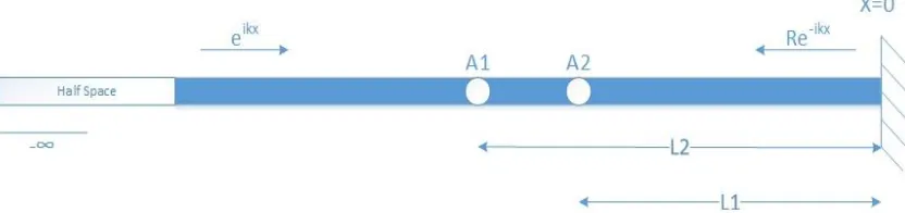
2.2.1 Experimental Wavenumber Analysis – Bar
We first illustrate the idea of experimental wavenumber in the simpler context of wave
propagation in a bar, truncated on the right and unbounded on the left.
A time-harmonic wave propagating forward from -∞ is represented by ikx
e and the reflected
wave is of the form ikx
Re where R is the reflection coefficient on the right (here time-variation of i t
e is implicitly assumed). The reflection coefficient R depends on the boundary condition on the right, and varies between 1 when completely free to -1 when completely fixed.
Thus the total displacement in the bar is given by
Re
ikx ikx
ue 2.11
The response at the accelerometer locations at distances L1 and L2 from the fixed end are given by
1 1
1 2
( ) ikL e ikL
u L u e R 2.12
2 2
2 1
( ) ikL e ikL
u L u e R 2.13
Substituting the above two expressions in equation 2.10 , the experimental wavenumber can
be computed. The plot of frequency versus experimental wavenumber is referred to as
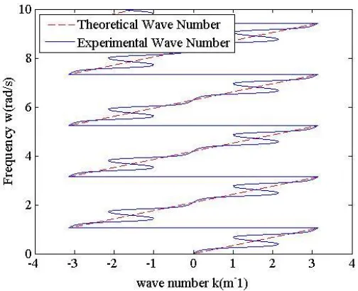
experimental dispersion curve. Figure 2.2 shows the theoretical and experimental dispersion curves for a bar with representative properties. Given the periodic nature of the definition of
experimental wavenumber in equation 2.10 the theoretical wave number is consistently
Figure 2.2: Theoretical vs Experimental Wave Number - Bar with L1=3m, L2=6m, c=1m/sec
It can be clearly seen from the above plot that the experimental wave number is periodic in
nature and contains wiggles, and can be explained by examining the expression for the
experimental wavenumber derived below.
We start with the ratio of the two displacements:
1
2 1 2
2
( )
2 2 1
R R
ikL
ik L L ikL
u e
e
u e
Taking logarithm of the ratio to find the experimental wavenumber, 1 2 2 2 2 2 1 1
log ( ) log( ikL R) log( ikL R)
a b
u
ik L L e e
u 2.15
To find the imaginary part of the equation 2.15, a and b are expanded separately as follows.
1
2
log( ikL R)
a e log cos(2
kL1) R isin(2kL1)
2.16Thus the imaginary part of a is the phase angle in the bracketed term:
1 1
1
sin(2 ) ( ) tan
cos(2 ) kL Imag a kL R 2.17
Similarly the imaginary part of b is given by
1 2
2
sin(2 ) ( ) tan
cos(2 ) kL Imag b kL R 2.18
Therefore the experimental wavenumber is given by
1 1 1 2
exp 2 1
1 2
1
2 3
sin(2 ) sin(2 )
( ) tan tan
cos(2 ) cos(2 )
kL kL
k k L L
R kL R kL
c c c 2.19
The periodic nature of kexpcan be explained using the terms c1, c2 and c3. In wavenumber
accelerometers. The period of c2and c3are dependent on lengths L1 and L2 respectively and are given by
1 2 ( ) Period c L 2.20 2 1 ( ) Period c L 2.21 3 2 ( ) Period c L 2.22
It can be seen from equation 2.19 that the slope of the experimental dispersion relation is
governed by c1 and the wiggles are jointly governed by c2and c3. The period of repetition of the group of wiggles is named as the cycle frequency and the period of the wiggles is named
as the wiggle frequency. Special case of R=-1 gives more insight into the experimental wavenumber.
1 1 1 2
exp 2 1
1 2
1 1
2 1 1 2
2 1 1 2
sin(2 ) sin(2 )
( ) tan tan
1 cos(2 ) 1 cos(2 )
( ) tan cot( ) tan cot( )
( )
2 2
0
kL kL
k k L L
kL kL
k L L kL kL
k L L kL kL
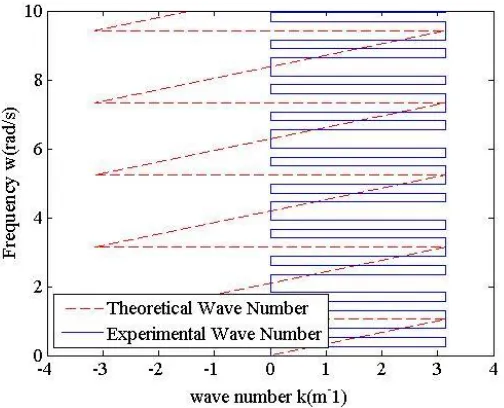
This result is evident, as there is absolute phase change of 180o at a perfectly fixed end. Figure
Figure 2.3: Dispersion Plot for a bar attached to half space on one end and perfectly fixed on other end
The cycle frequency and wiggle frequency can be obtained experimentally and they depend on
L
and L1,L2respectively. The cycle and wiggle frequencies are given by
Cycle frequencies = 2 L
2.23
Wiggle frequencies = LCM of
1
L
and
2
L
2.24
The above definition of the wiggle frequency is valid only for integer values of L1 and
2
L
. But nevertheless an estimate for the length can be found using the wiggle frequency
error. The other important observation is that, the number of wiggles in each cycle is constant,
i.e. for a given system the ratio of the cycle and wiggle frequency is a constant given by
Ratio of cycle and wiggle frequency = 2 L 2L
L L
2.25
The only unknown in equation 2.25 is the length L and an estimate can be obtained without
any need for the information about the material properties of the bar and this can be
advantageous for easy and quick nondestructive evaluation.
2.2.2 Experimental Wavenumber Analysis – Beam
The analysis becomes more involved for a beam due to the existence of evanescent modes of
waves. The solution for the governing equation for a beam given in equation 2.4 in frequency
domain is given by
1 1 2 2
1 2 3 4
( ) C ik x C ik x C k x C k x
y x e e e e 2.26
where k1,k1,ik2, i k2are the roots of equation 2.6. Thus the ratio of response at the two accelerometer locations is
1 1 1 1 2 1 2 1
1 2 1 2 2 2 2 2
1 2 3 4
1 2 3 4
C C C C
C C C C
ik L ik L k L k L
ik L ik L k L k L
e e e e
ratio
e e e e
2.27
There are two new terms corresponding to the evanescent modes along with the propagating
modes. The distance between the impact and the accelerometer can be chosen to damp out the
evanescent modes of the response, thus obtaining a response dominated by the propagating
the beam and the results can be extended. The following two conditions are ideal for using the
bar formulations for the beam analysis
Impact location is sufficiently far away from the accelerometer location so that the
evanescent modes are damped out.
The distance between the two accelerometers is small enough so that the wiggles are
periodic. If the two lengths (lengths to the accelerometers from the pile tip) are close
to each other, the length estimate from the period of the wiggles has less error.
The above two conditions are easy to achieve in pile foundation testing setup. The evanescent
modes are further damped to material damping as well as radiation of the waves into the soil
surrounding the pile. Even in cases in which the evanescent mode effects are significant, they
are confined only to the lower frequencies.
The dispersion relation for a beam i.e. the relation between and k is parabolic, but is linear for a bar. Thus the modified dispersion plot of wavenumber vs the square root of the frequency(
w ) is considered, which makes the relation linear and facilitates direct extension of the results obtained from the bar analysis. The wiggle frequency given in equation 2.24 can be
used to find the length scale of the system. The cycle frequency is used to obtain the material
2 w
L cr
2.28
2 2 24
w L
c
r
2.29
During certain experiments it is possible that even one full cycle cannot be captured and thus
cycle frequency is unknown. Characteristic material properties can be used in these cases to
find the length estimate from the wiggle frequency.
2.3 Pile Foundation – Embedded Length Estimation
Pile foundation can be modelled as a Bernoulli-Euler beam for nondestructive evaluation
purposes, due to its inherent slenderness and low impact.The beam experimental wavenumber
analysis results shown in section 2.5 can be used to estimate the length and young’s modulus
of the pile foundation.
This analysis technique does not take into account the soil effect and is purely based on
matching the dispersion relation. The estimated properties can be used as a starting point if an
inversion based technique is used, efficiency of which depends highly on the initial guess. Soil
can be beneficial in this analysis as it damps out the evanescent waves faster with the signal
2.4 Numerical Examples
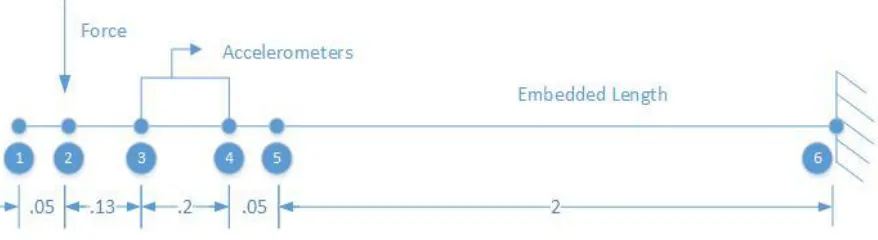
The properties of a prototype pile installed in Northwestern University for the work done by
Lynch [3] has been considered for all the theoretical analysis done in this work. The pile has
properties shown in Table 2-1 and the experimental setup is shown in Figure 2.4 below.
Table 2-1: Prototype Pile Properties
Pile C355-2430
Length (m) 2.43
Radius .178
Young’s Modulus (GPa) 35.7
Shear Modulus (GPa) 15.04
Density 2350
Poisson’s Ratio .20
Shear Wave Velocity 2530
Bar Wave Velocity 3900
Surrounding Soil Poisson’s ratio .3 Surrounding Soil Shear Modulus (GPa) .01719 Surrounding Soil Young’s Modulus (GPa) .04464
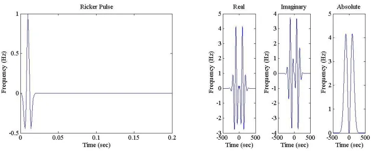
The Ricker pulse was chosen as the forcing function for the synthetic examples. The Ricker
pulse is controlled by the forcing frequency f0 and the start timet0 is given as1 f0. The expression is given by
2 2 20( 0)
2 2 2
ker 1 2 0 ( 0)
f t t ric
F f tt e 2.30
Figure 2.5 shows a Ricker pulse with a forcing frequency of 100Hz.
Figure 2.5: Ricker Pulse of 100 Hz forcing frequency
The experimental wave number is obtained from equation 2.10 and plotted against to find
the wiggle and cycle frequencies. The first of the two examples shows the results from the pile
with the same setup shown in Figure 2.4. The dispersion curve for this example is shown in
Figure 2.6 and the resulting length estimate and associated error are shown in Table 2-2. In the
accelerometers is increased to .5m. Figure 2.7 contains the dispersion curve and Table 2-3
contains the associated results. In both these examples, the experimental wave number analysis
works well, especially when the modulus is known.
Figure 2.6: Experimental wave number plot for Free-Fixed Pile example 1
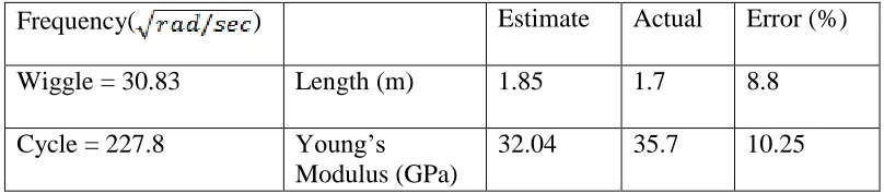
Table 2-2: Length Estimation and Error for Example 1
Frequency( ) Estimate (m) Actual (m) Error (%)
Wiggle = 27.495 Length 2.08 2 4
Figure 2.7: Experimental wave number plot for Free-Fixed Pile example 2
Table 2-3: Length and Young’s Modulus, Estimation and Error for Example 2
Frequency( ) Estimate Actual Error (%)
Wiggle = 30.83 Length (m) 1.85 1.7 8.8
Cycle = 227.8 Young’s
Modulus (GPa)
32.04 35.7 10.25
on the parameters needed to be estimated from testing, distance between the accelerometers
should be designed.
Gaussian noise with signal to noise ratio (SNR) 103 is added to the response from a setup same
as example 1. The polluted signal shown in Figure 2.8(a) is processed for the experimental
wave number, which is shown in Figure 2.9(a), which is understandably less periodic than
noise-free dispersion plot The results from this noise-laden dispersion curve is shown Table
2-4. Fortunately, the results are quite encouraging even in the presence of noise. However,
when the SNR is decreased to 102, the results are not encouraging (as shown in Figure 2.8(b),
Figure 2.9(b) and Table 2-5).Preliminary filtering techniques based in frequency windowing
were not successful and further effort is necessary in this direction.
(a)
(b)
Table 2-4: Length Estimation and Error for signal with Gaussian SNR 103
Frequency( ) Estimate (m) Actual (m) Error (%)
Wiggle = 27.52 Length 2.08 2 4
Table 2-5: Length Estimation and Error for signal with Gaussian SNR 102
Frequency( ) Estimate (m) Actual (m) Error (%)
Wiggle = 25.23 Length 2.27 2 13.5
2.5 Discussion
A new signal processing technique has been introduced to nondestructively estimate the
properties of bars and beams, which requires excitation of the system using an impact and
recording the response at two locations along the length which is to be determined. The
experimental wavenumber is obtained from the experimental response and compared with the theoretical wavenumber to estimate the length and young’s modulus. The technique is applied
for a pile foundation to estimate these two parameters from the response due to a lateral impact.
The distance between the accelerometers is the most important parameter in this technique, as
it governs the accuracy of the estimates and also the amount of information that can be obtained
from the data. Placing the accelerometers close to each other gives more accurate results for
the length, but most often does not contain information to evaluate the material property.
young’s modulus of the pile, but reduces the accuracy of the results. Having more
accelerometers would potentially increase the accuracy of the results, but requires further
development of the data analysis procedure. This proposed technique is still in its developing
3 EFFECT OF SOIL ON FLEXURAL WAVE PROPAGATION AND PREDICTION OF LENGTH AND YOUNG’S MODULUS
The pile and soil form a system with majority of the pile embedded in the soil. The soil
surrounding the pile has significant effect on the behavior of the pile at particular frequency
ranges. A large portion of the wave generated from impact is attenuated due to the presence of
soil, which can be both advantageous and disadvantageous. The attenuation reduces the
amplitude of the reflected wave and thus makes obtaining a signal with high signal to noise
ratio (SNR) difficult. At the same time modelling of soil is very important to improve the
efficiency of the model to represent the actual conditions and more so, when an optimization
based approach is implemented for NDE of the pile foundation. This chapter develops the soil
model which will be used to modify the Bernoulli-Euler beam model and the modified model
is used for optimization of the pile parameters.
3.1 Introduction
There have been multiple works trying to estimate the effect of soil in various conditions. The
dynamic modelling can be classified broadly under three methods [7], (a) Dynamic
Winkler-foundation approach (b) Elastic continuum methods and (c) Dynamic finite element
formulation.
The Winkler foundation based models are easy to implement of the three. They are based on
estimating the soil stiffness using linear horizontal and vertical springs, and dashpots. This
represents material and hysteretic damping. The earliest models of this type used static theory
introduced the first model that included the radiation damping effects, and this model assumed
that the tip of the pile is embedded in rigid bedrock and the soil around the pile is made of
infinitesimally thin, horizontal layers. This work has considered horizontal and translational stiffness offered by the soil and hasn’t considered the rotational effects. More sophisticated
analysis techniques using p-y curves have also been used to model the Winkler foundations
incorporating nonlinear springs [9-12]. All the analysis mentioned above has been mainly
developed for seismic response of the pile and not in the context of NDE. Since the impact is
in the elastic region, elastic modeling of the soil can still be used and more sophisticated
techniques are not needed.
The Elastic continuum methods consider soil as a continuous elastic or viscoelastic medium
and calculate the displacements from point load within the half space to obtain analytic solutions. The infinite extent of the continuum allows for closed form solutions for the Green’s
functions [13-19]. Boundary element method (BEM) uses boundary integral equations to
model soil behavior in the time or frequency domain [20-23]. Discretization of the pile-soil
boundary is required, and, depending on the type of Green’s functions that are used, sufficient
discretization of the free surface may also be needed. This analysis technique is more accurate
than the Winkler foundation model, but introducing layered soil or varying elastic moduli introduces significant complexity in finding the Green’s functions.
Finite element (FE) models are versatile and allow incorporation of nonlinear behaviors of the
soil properties and the interface between soil and pile [24-28]. Dynamic FE models require
Discretizing a huge volume of soil might become computationally intensive and inversion
using this model will subsequently become more difficult.
This work includes the effect of soil using an approximate analytical method, estimating both
translational and rotational resistance offered. Rotational resistance has not been considered
earlier and can have significant effect in low frequency. Though translational stiffness of soil
estimated using this technique has been used earlier, it has not been used in the context of
NDE. A typical impact test requires excitation of the pile from an impulse and the stresses
generated are much less than the yield stress of the material. Thus the elastodynamic analysis
results can be conveniently used for modeling. Also an inversion based optimization
methodology to find the pile parameters is introduced in this work.
3.2 Dispersion Relation
The dispersion relation relates the wavenumber to the frequency and can be used to obtain
phase and group velocities. Considering slender piles, we utilize Bernoulli-Euler beam model to obtain the dispersion relation. Assuming a beam with Young’s modulus E, Density , Moment of Inertia I and cross sectional area A, the fourth order equation governing wave propagation without any external forces is given by
4 2
4 2 0,
y y
EI A
x t
3.1
ikx i t
ye 3.2
where is the frequency and k is the wavenumber. Substituting equation 3.2 in the governing equation, the dispersion relation can be obtained.
4 2
0
EIk A 3.3
k cr
3.4
where c E is the bar wave velocity and r I Ais the radius of gyration.
Phase velocity is defined as the ratio of the frequency to wavenumber, and the group velocity
is defined as the derivative of the frequency with respect to wavenumber. Graphically at any
point in the dispersion curve, phase velocity is given by the secant and group velocity is the
tangent to the curve. They are given by the following expressions for a Bernoulli-Euler beam,
phase
C rc
k
3.5
2
group
d
C rc
dk
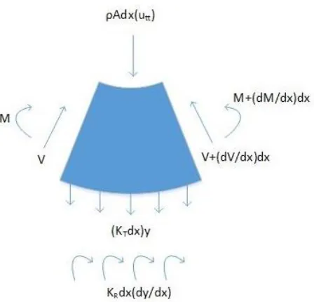
3.3 Modified Flexural wave model
The modified flexural wave model is obtained by adding the translational and rotational
stiffness offered by the soil. The differential element with the addition of the effect from the
soil is shown below.
Figure 3.1: Differential Beam element with translational and rotational springs
The governing equation has two new terms compared to the basic Bernoulli-Euler beam due
to the soil effects as follows.
4 2 2
4 R 2 T 2 0
y y y
EI K K y A
x x t
3.7
4 2 2
( ) 0
R T
EIk K k K A 3.8
which is used in Section 3.5 to examine the effect of soil on wave propagation characteristics,
and thus on prediction of embedded length.
3.3.1 Stiffness Matrix Method to capture the effect of Soils
Additionally, in section 3.6, we propose an optimization technique to predict the lengths that
depend on matching the measured responses. This is performed with the help of stiffness
matrix method that captures the soil effects. In this section, we derive an element stiffness
matrix of a beam element of length L shown in Figure 3.2. The solution takes the form,
3
1 2 4
1 2 3 4
ik x
ik x ik x ik x
yC e C e C e C e 3.9
where k k k k1, 2, 3, 4 are the four solutions of the dispersion relation in equation 3.8. Equation 3.9 can be written in a matrix form as
1 2 3 4
1 2 3 4 ik x
ik x ik x ik x
C C
y e e e e
C C
Figure 3.2: Beam element with nodal forces
The displacements and rotations at the two nodes are given by
1 0 2 0 3 4 ' ' x x x L x L y y y y y y y y 3.11 3
1 2 4
3
1 2 4
1 1
1 2 3 4
2 2
3 3
1 2 3 4
4 4
1 1 1 1
ik L
ik L ik L ik L
ik L
ik L ik L ik L
y C
ik ik ik ik
y C
e e e e
y C
ik e ik e ik e ik e
y C 1 T 3.12
3 3 0 2 0 1 0 2 1 0 3 2 3 2 2 2 0 0 x x x x L x R x L x L
x L x L
x L y EI x y y V F x EI x M M K V
F y y
EI M
M x x
y EI x 3.13 3
1 2 4
3
1 2 4
3 3
1 1
3 3
1 2 3 4
2 2 2 2
1 2 3 4
3 3 3 3
1 2 3
1 2
2 4 3
2 2 2 2
1
2 2 3 4 4
ik L
ik L ik L ik L
ik L
ik L ik L ik L
F C
M C
F C
M C
ik ik ik ik
k k k k
EI
ik e ik e ik e ik e
k e k e k e k e
2 T 3
1 2 4
1 2 1
2 3 4
3 4
1 2 3 4
0 0 0 0
0 0 0 0
ik L
ik L ik L ik
R L
ik ik ik ik
ik e ik e ik e i
C C K C k C e 3 T 3.14
Equation 3.12 can be rearranged to get
1 1
2 1 2
1 1
1 1 2
2 3
2 4
R
F y
M y
EI K
F y
M y
2 3 1
T T T
3.16
1 1
R
K EI K
T T2 1 T T3 1 3.17
The above expression gives the stiffness matrix of a beam with soil effects, which can in turn
be to model the soil pile system. The rotational and translational stiffness offered by soil is
derived in the next section.
3.4 Derivation of soil stiffness
The soil can be viewed as infinite domain, with a cylindrical hole created by the pile. Making
the assumption of homogeneity, the waves will follow the three-dimensional elastodynamic
equation. Considering that the length of the pile and the wavelength of flexural waves are large
compared to the diameter, we utilize plane elasticity assumption in the horizontal plane,
decoupling plane and in-plane components of the deformation. Soil resistance from
anti-plane deformation can be modeled through rotational springs, while in-anti-plane resistance can be
modeled through translational springs. The details are described below.
2 2 2
2 2 2 2
1 1
0
u u u u
r r r r t
3.18
Owing to the cylindrical geometry of the pile, the solution can be written as superposition of
wave modes,
( , , ) (r) cos( ) i t
u r t U e 3.19
which reduces the equation to
2 2 2 2 1 1 0 s U U U
r r r C r
3.20
where,Cs
is the shear wave velocity. Substitutingr r c
, the above equation reduces
to a standard Bessels equation with Hankel functions as solutions,
1 2
1 1
( )
s s
r r
U r AH BH
C C 3.21
Where, 1
( )
n
H z and 2
( )
n
H z are respectively the 1st and 2nd kind of Hankel functions of order n.
Applying radiation conditions at infinity, the solution takes the form
1 1
( )
s
r U r AH
1 1
( , , ) cos( ) i t
s
r
u r t AH e
C
3.23
Figure 3.3: Unit Rotation of the Pile
To obtain the rotational stiffness effect of the soil on the pile, we apply unit rotation of the pile
section and compute the overall resisting moment from the resulting traction on the circular
boundary:
Unit Rotation u R( , ) cos( ) 3.24
1 1
cos( ) cos( )
s
R AH
C
1 1 1 A s R H C 3.26
Therefore the final solution from equation 3.20 is,
1 1 1 1 cos( ) ( , ) s s r
u r H
C R H C 3.27
The stress acting at rRis given by
n r R u G r 3.28 1 0 1 1 1
cos( ) s
s s R H C G R R C H C 3.29
The resulting moment is given by the integral,
2
0
R cos( )
R n
K Rd
3.30Given that unit rotation is applied, the above expression for resisting moment is essentially the
rotational stiffness. Clearly, the rotational stiffness is a function of the soil properties and the
frequency.
3.4.2 Translational Stiffness for Plane-Strain Deformation
The In-plane wave equation in terms of scalar () and vector ( ) potentials governs the wave
propagation in the (r,) plane given by
2 22
2 d 0
dt
3.32
2 2 2 0 t ψ ψ 3.33where the scalar and vector potentials are defined as,
0 T
u ψ ψ 3.34The solution to Equation 3.32 is given by
1 2
1 1
( )
p p
r r
r AH BH
C C
3.35
where Cp 2
Similar to equation 3.21, applying radiation boundary conditions,
1 1
( ) cos( )
p
r
r A H
C
3.36
Using a similar procedure, we have the solution for the vector potential as
1 1
( ) sin( )
s
r H r
C
C
ψ 3.37
Applying unit translation at the pile-soil interface, we have,
1, 0
x y
u u 3.38
The polar representation of the displacement boundary condition is, cos( ) sin( ) r r R u u 3.39
which can be used to obtain the coefficients A and C in Equations 3.36 and3.37:
1 1
0 1
1 1 1 1 1 1
0 0 0 1 1 0
1 1 0 1 1 0 2 2 p s s s p s
s p s p s p
s
p
p p
s
C R R
H R C H
C C
A
R R R R R R
R H H C H H C H H
C C C C C C
C R R
H R C H
C C
C
R
R H H
C
1 1 1 1 1
0 p 1 0 s 1 0
p s p s p
R R R R R
C H H C H H
C C C C C
3.40
The stresses can be evaluated using the strain displacement relation and the constitutive
relation 2 ( ) 2 0 1 0 cos 1 1 0 sin 1 0 0 1 1 ( ) rr r r r r r r r r
r r r
3.41
cos( ) sin( )
rr r R
r r R
M N 3.42 where, 2
2 2 2
( 2 ) 2 2
r R
M
r r r r r r r
3.43 2
2 2 2
2 2 1
r R
N
r r r r r r r
3.44
The translational stiffness is the force at a distance R given by
2 2
0 0
cos( ) sin( )
T rr r
K R Rd R Rd
3.45Using equations 3.43 and 3.44, the above expression simplifies to
( )
T
K R MN 3.46
2
2 1 1
1 1 ( ) T p s K R r r
R AH H
C C C
3.47
which is the frequency dependent translational stiffness. As an example, the rotational and
(a)
(b)
At zero frequency, the rotational and translational stiffness represent the stiffness of the static
case. The rotational stiffness reaches a maximum value of G R at zero frequency and the translational stiffness has a value of zero at zero frequency. This counter intuitive behavior of
the translational stiffness is further studied using the static case and associated mathematical
proof and derivations can be found in appendix A.
3.5 Effect of soil on dispersion relation
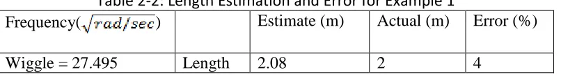
The effect of the soil is further illustrated in Figure 3.6 and Figure 3.7, where the dispersion
relations are compared for the cases with and without soil for a soft soil and stiff soil
respectively. The dispersion relation clearly shows the difference in the dispersion curves of
the free and embedded cases (solid and dotted lines respectively). The effect is most felt only
in the low frequencies typically up to maximum 5000Hz in very stiff soil profiles. The upper
limit of the effect depends on the relative properties of the soil and the pile. A pile embedded
in hard soil has soil effects running higher in the frequency range than that of the pile in a soft
soil. In a typical test in which a pile is impacted on the side, only low frequencies are excited.
This frequency content depends on the hammer head material, pile material and the impact
time. Thus effect of soil cannot be ignored in these tests and needs to be captured to the
(a)
(b)
Figure 3.6: Dispersion Relation with dotted lines showing the embedded pile and solid lines representing the free pile for reference for a pile of radius .178m and soil with
(a)
(b)
Figure 3.7: Dispersion Relation with dotted lines showing the embedded pile and solid lines representing the free pile for reference for a pile of radius .178m and soil with
3.6 Inversion
Inversion is a process of back calculating the unknown parameters of a system from the
response of the system. The main objective in our context is to find the length and Young’s
modulus of the pile using the response obtained from an impact test. Response obtained at the
accelerometer locations from the experiment is compared to that obtained from the flexural
wave model developed, to optimize for the length and Young’s modulus of the pile.
The objective or misfit function, incorporating both the model and experimental response is
minimized to find the optimum parameters. A one dimensional beam model developed in the
previous sections is used as the forward model. The signal from actual experiments will contain
noise that needs to be filtered before the optimization process. Frequency spectrum based
filters such as Butterworth filter can be used to smoothen the signal in the time domain.
The objective function is chosen as the Euclidian norm of the difference between the
experimental and model response and is given by
mod obj exact el
F u u 3.48
where, uexactis the experimental response and umodelis the model response.
The choice of parameters is important as the behavior of the objective function is dependent
on them. The main system information of interest from optimization, are the length and the Young’s modulus of the pile foundation. Two sets of parameters are chosen, (1) Length and
Young’s modulus and (2) Length and ratio of length to bar wave velocity c, which is the ratio
function of these parameters is studied. The low dimensional parameter space allows us to
inspect the objective function by plotting it as a function of the two parameters.
Two scenarios arise due to the experimental set-up and conditions based on the known
information from the testing as follows,
Forcing and response at both the accelerometer locations are known – The impact
device used in this method is capable of recording the force imparted during impact.
Only the response at both the accelerometer locations are known – The force
imparted from impact is not recorded.
The forward model has been developed in a matrix framework mainly because the response at
discrete locations along the length of the pile are sought after. This can be used as an advantage
in the case when the information on the forcing function is not available, the matrix formulation
can be rearranged to use the response at one accelerometer location to find the response at the
other accelerometer locations. Numerical examples for different cases are shown in the
following section.
3.7 Numerical Examples
The properties of a prototype pile installed in Northwestern University for the work done by
Lynch [3] has been considered for all the theoretical analysis done in this work. The pile has
Table 3-1: Prototype Pile Properties
Pile C355-2430
Length (m) 2.43
Radius .178
Young’s Modulus (GPa) 35.7
Shear Modulus (GPa) 15.04
Density 2350
Poisson’s Ratio .20
Shear Wave Velocity 2530
Bar Wave Velocity 3900
Surrounding Soil Poisson’s ratio .3 Surrounding Soil Shear Modulus (GPa) .01719 Surrounding Soil Young’s Modulus (GPa) .04464
Figure 3.8: Prototype Pile Properties
The Ricker pulse was chosen as the forcing function for the synthetic examples. The Ricker
2 2 2 0( 0)2 2 2
ker 1 2 0 ( 0)
f t t ric
F f tt e 3.49
Figure 3.9 shows a Ricker pulse with a forcing frequency of 100Hz.
Figure 3.9: Ricker Pulse of 100 Hz forcing frequency
3.7.1 Experimental Wavenumber Analysis – Comparison between free, fully embedded and partially embedded pile
The experimental wavenumber analysis described in the previous chapter is applied for three
cases, (1) free pile (2) fully embedded pile and (3) partially embedded pile, and the results are
compared. Soil has a positive effect on the analysis, as the evanescent waves are damped faster
(a) (b)
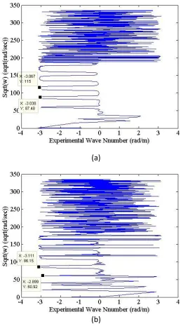
(c)
Figure 3.10: Experimental Dispersion relation (a) Fully Embedded Pile (b) Partially Embedded Pile (c) Free Pile
Table 3-2: Comparison of Free, Fully Embedded and Partially embedded cases Free Pile Fully Embedded Partially Embedded Wiggle Frequency
(rad/sec)
25.25 27.91 27.91
Estimated Length (m) 2.27 2.05 2.05
Actual Length 2 2 2
3.7.2 Inversion to find the length and material parameters
The behavior of the objective function defined in equation 3.48 with respect to the length, young’s modulus and the ratio of length to bar wave velocity are explored Figure 3.11, Figure
3.12 and Figure 3.13. Local minimas are observed but the solution at the global minimum
corresponds to the exact solution. Also it can be observed that the variation of the objective
function is smoother when L and L/C are considered as parameters.
Figure 3.12: Objective function as a function of length L and Young’s modulus E
Table 3-3: Minimum and Error for Length and Young’s Modulus
Parameters Minimum Exact Error (%)
Length L (m) 2 2 0
Length & Young’s Modulus
L (m) 2 2 0
E (Pa) 35.84e9 35.7e9 .39
Length & Ratio of Length and
Bar Wave Velocity
L (m) 2 2 0
L/C (sec) .512 .5131 .214
3.7.3 Effect of Soil in Inverting for the length
The effect of soil can be significant and can affect our inversion process, resulting in
completely wrong estimates of the parameters. Figure 3.14(a) and (b) shows the objective
function as a function of length, without adding soil effects and with soil effects respectively
and Table 3-4 shows the error between the global minima and the exact solution. Due to ignoring the soil effects, lot of local minima’s can be observed and the global minima occurs
at 2.8m, where the exact length is 2m. This trend is not observed when the soil effects are
included as the global minimum is the same as the exact solution. Thus ignoring soil effects
(a) (b)
Figure 3.14: Comparison of objective function with and without including soil effects
Table 3-4: Comparison of error with and without including soil effects
Minimum (m) Exact (m) Error (%)
Optimization without soil effects
(a)
2.8 2 40
Optimization with soil effects (b)
2 2 0
3.8 Conclusion
Effect of soil has been captured using translational and rotational springs, stiffness of which
has been calculated by solving the three dimensional elastodynamic wave equation using
Helmholtz decomposition. Helmholtz decomposition decouples the three dimensional wave
domain. It is important to note that the obtained stiffness is a function of frequency and the soil
properties.
Modified flexural wave model is developed to obtain the response at the accelerometer
locations, which includes the effect of soil on the wave propagation in the pile. Inversion based method has been explored to find the embedded length and Young’s modulus of the pile
foundation using the improved model. The theoretical results presented show less error in the
estimated parameters. In cases where the soil properties are not known to high accuracy,
representative properties can be used, based on whether the soil is dense or loose packed and
the location.
The model developed has been tested only on synthetic data and needs to be validated using
real data from lab experiments. Frequency spectrum based filters such as Butterworth filter can
be used to smoothen the time domain signal, which can improve the inversion process. More
rigorous analysis and effective noise handling techniques need to be explored. Also ideal soil
conditions are assumed and the model needs to be extended to saturated and more complex
soil conditions. The model has been developed for homogeneous soil but the results can be