University of Windsor University of Windsor
Scholarship at UWindsor
Scholarship at UWindsor
Electronic Theses and Dissertations Theses, Dissertations, and Major Papers
2013
Testing and improving local adaptive importance sampling in LJF
Testing and improving local adaptive importance sampling in LJF
local-JT in multiply sectioned Bayesian networks
local-JT in multiply sectioned Bayesian networks
Sonia Bhatti
University of Windsor
Follow this and additional works at: https://scholar.uwindsor.ca/etd
Recommended Citation Recommended Citation
Bhatti, Sonia, "Testing and improving local adaptive importance sampling in LJF local-JT in multiply sectioned Bayesian networks" (2013). Electronic Theses and Dissertations. 4725.
https://scholar.uwindsor.ca/etd/4725
TESTING AND IMPROVING LOCAL ADAPTIVE IMPORTANCE
SAMPLING IN LJF LOCAL-JT IN MULTIPLY SECTIONED BAYESIAN
NETWORKS
By
SONIA BHATTI
A Thesis
Submitted to the Faculty of Graduate Studies through the School of
Computer Science in Partial Fulfillment of the Requirements for the Degree
of Master of Science at the
University of Windsor
Windsor, Ontario, Canada
2012
TESTING AND IMPROVING LOCAL ADAPTIVE IMPORTANCE
SAMPLING IN LJF LOCAL-JT IN MULTIPLY SECTIONED BAYESIAN
NETWORKS
by
SONIA BHATTI
APPROVED BY:
______________________________________________ Dr.Yunbi An, External Reader
Odette School of Business
______________________________________________ Dr. Yung H.Tsin, Internal Reader
School of Computer Science
______________________________________________ Dr. Dan Wu, Advisor
School of Computer Science
______________________________________________ Dr. Hongxuan(Karen) Jin, Co-Advisor
School of Computer Science
______________________________________________ Dr. Imran Ahmad, Chair of Defense
School of Computer Science
Declaration of Originality
I hereby certify that I am the sole author of this thesis and that no part of this thesis has been
published or submitted for publication.
I certify that, to the best of my knowledge, my thesis does not infringe upon anyone’s
copyright nor violate any proprietary rights and that any ideas, techniques, quotations, or any
other material from the work of other people included in my thesis, published or otherwise,
are fully acknowledged in accordance with the standard referencing practices. Furthermore,
to the extent that I have included copyrighted material that surpasses the bounds of fair
dealing within the meaning of the Canada Copyright Act, I certify that I have obtained a
written permission from the copyright owner(s) to include such material(s) in my thesis and
have included copies of such copyright clearances to my appendix.
I declare that this is a true copy of my thesis, including any final revisions, as approved by
my thesis committee and the Graduate Studies office, and that this thesis has not been
Abstract
Multiply Sectioned Bayesian Network (MSBN) provides a model for probabilistic reasoning
in multi-agent systems. The exact inference is costly and difficult to be applied in the context
of MSBNs. So the approximate inference is used as an alternative. Recently, for reasoning in
MSBNs, LJF-based Local Adaptive Importance Sampler (LLAIS) has been developed for
approximate reasoning in MSBNs. However, the prototype of LLAIS is tested on Alarm
Network (37 nodes). But further testing on larger networks has not been reported. In this
thesis, LLAIS algorithm is tested on three large networks namely Hailfinder (56 nodes),
Win95pts (76 nodes) and PathFinder (109 nodes), to measure for its reliability and
scalability. The experiments done show that LLAIS without parameters tuned shows good
convergence for Hailfinder and Win95pts but not for Pathfinder network. However, when the
parameters are tuned the algorithm shows considerable improvement in its accuracy for all
the three networks tested.
Acknowledgment
First of all, I would like to thank my supervisor Dr. Dan Wu for advising and supporting me
throughout the thesis with his patience and knowledge. I have learned a lot under his
guidance, he always guided me in understanding the problem and giving me the way to find
its solution. I was naïve when he took me under his supervision but he taught me how to set
standards for myself so that I could improve myself. Dr. Karen H. Jin, Lecturer in
Department of Computer Science, University of New Hampshire, USA, who guided me in
spite of being outside the University of Windsor. She gave her valuable time and unselfish
support throughout the thesis work.
I offer my sincere gratitude to Dr. Dan Wu and Dr. Karen H Jin, without them my thesis
would never have been completed or written.
I would also like to thank my external reader, Dr. An, my internal reader, Dr. Tsin, and my
thesis committee chair, Dr. Ahmad, for making time to be in my thesis committee, reading
the thesis and providing valuable input. I appreciate all your suggestions, which have helped
improve the quality of this thesis.
In my daily work I have been blessed with a friendly and cheerful group of fellow students,
want to thank them for their friendship, kindness and moral support.
I would like to express my gratitude to my parents for their prayers and endless love, paying
my tuition fee and giving me the opportunity to study in University of Windsor and in the end
Table of Content
Declaration of Originality ... iii
Abstract ... iv
Acknowledgment ... v
List of Figures... viii
List of Tables ... x
1. Introduction ... 1
1.1 Motivation ... 1
1.2 Objective ... 4
1.3 Overview of Thesis... 6
1.4 Thesis Contribution ... 7
2. Background Study ... 9
2.1 Concepts in Probability... 9
2.1.1 Probability Theory ... 9
2.2 Probabilistic Graphical Models ... 11
2.3 Dependency Model ... 13
2.4 Bayesian Network - Definition and Example ... 14
2.5 Inference in Bayesian Networks ... 16
2.5.1 Exact Inference ... 17
2.5.2 Approximate Inference ... 20
2.6 Sampling in BN ... 23
2.6.1 Mathematical Foundation for Importance Sampling ... 25
2.6.2 Importance Sampling for BN ... 27
2.7 Multiply Sectioned Bayesian Network (MSBN) ... 30
2.8 Linked Junction Tree Forests (LJFs) in MSBNs ... 34
2.8.1 Initialization of LJF ... 36
2.9 Inference in MSBN... 38
2.9.1 Importance Sampling for LJF local-JT ... 40
2.10 Discussion ... 44
3. Adaptive Importance Sampling in Bayesian Network ... 45
3.1 Adaptive Importance Sampling in BN ... 45
3.1.1 Algorithm for AIS-BN ... 46
3.2 LJF Local Adaptive Importance Sampling ... 48
3.2.1 Algorithm for LLAIS ... 49
3.3 Discussion ... 50
4. Methods for Testing and Improving LLAIS ... 51
4.1 Motivation ... 51
4.2 Network Selection ... 52
4.3 Experiments for Testing LLAIS ... 53
4.3.1 Performance Measures ... 53
4.3.2 Example for Testing Procedure ... 55
4.3.3 Design of Experiment ... 60
4.4 Improving LLAIS by Tuning the Tunable Parameters ... 61
4.5 Method for Testing the Improved LLAIS... 65
4.5.1 Design of Experiment ... 65
4.5.2 Performance Measure ... 66
5. Experiment Results for Testing and Improving LLAIS ... 68
5.1 Testing of LLAIS ... 68
5.2 Experiment Results ... 69
5.2.1 Testing Results on Hailfinder BN ... 70
5.2.2 Testing Results on Win95pts BN ... 77
5.2.3 Testing Results on Pathfinder BN ... 85
5.3 Summary of Testing ... 93
5.4 Tuning the Parameters and Improving LLAIS ... 94
5.5 Experiment Results ... 95
5.5.1 Experiment Results for Improved LLAIS on Hailfinder BN ... 95
5.5.2 Experiment Results for Improved LLAIS on Win95pts BN ... 97
5.5.3 Experiment Results for Improved LLAIS on Pathfinder BN... 99
5.6 Summarizing the Experiments in terms of Time Taken ... 101
5.7 Discussion ... 104
6. Conclusion ... 105
6.1 Thesis Summary ... 105
6.2 Future Work ... 107
Bibliography ... 108
Vita Auctoris ... 113
List of Figures
Figure 2.1: The Asia Travel Network-simple BN ... 16
Figure 2.2: The Graph G in (a) is sectioned into and in (b) ψ in (c) is a hypertree over G ... 34
Figure 2.3: (a) A BN (b) A small MSBN with three subnets (c) the corresponding MSBN hypertree ... 36
Figure 2.4: An MSBN LJF shown with initial potentials assigned to all the three subnets.. ... ….37
Figure 2.5: Inter-agent message passing ... 39
Figure 2.6: Sampling local JT with {abc} as root... 43
Figure 4.1: Procedure for testing LLAIS... 59
Figure 5.1: Steps for testing LLAIS on larger networks ... 69
Figure 5.2: Structure of Hailfinder Network with 56 nodes and 66 edges... 70
Figure 5.3: Performance comparison of approximate importance function and exact importance function on Hailfinder network with 9 evidence nodes ... 71
Figure 5.4: Performance comparison of approximate importance function and exact importance function on Hailfinder network with 11evidence nodes ... 72
Figure 5.5: Performance comparison of approximate importance function and exact importance function on Hailfinder network with 13 evidence nodes ... 73
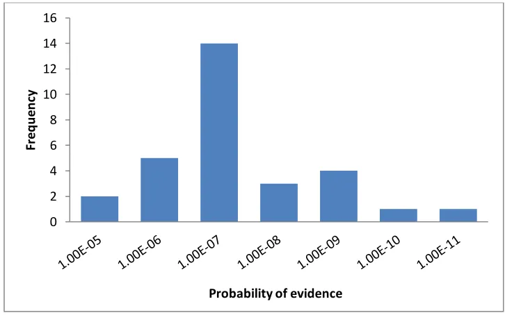
Figure 5.6: Frequency distribution of P(E) in Hailfinder network ………...74
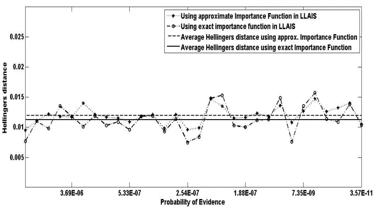
Figure 5.7: Performance comparison of approximate and exact importance function combining all the 30 test cases generated in terms of Hellinger's distance for Hailfinder network ... 75
Figure 5.8: Performance comparison of approximate and exact importance function combining all the 30 test cases generated in terms of Mean Square Error for Hailfinder network. ... 77
Figure 5.9: Structure of Win95pts network with 76 nodes and 112 edges ... 78
Figure 5.10: Performance comparison of approximate importance function and exact importance function on Win95pts network with 9 evidence nodes ... 79
Figure 5.12: Performance comparison of approximate importance function and exact importance function on Win95pts network with 13 evidence nodes ... 81
Figure 5.13: Frequency distribution of P(E) in Win95pts network ... 81
Figure 5.14: Performance comparison of approximate and exact importance function combining all the 30 test cases generated in terms of Hellinger's distance for Win95pts network ... 83
Figure 5.15: Performance comparison of approximate and exact importance function combining all the 30 test cases generated in terms of Mean Square Error for Win95pts network ... 84
Figure 5.16: Structure of Pathfinder network with 109 nodes ... 85
Figure 5.17: Performance comparison of approximate importance function and exact importance function on Pathfinder network with 9 evidence nodes ... 86
Figure 5.18: Performance comparison of approximate importance function and exact importance function on Pathfinder network with 11 evidence nodes ... 87
Figure 5.19: Performance comparison of approximate importance function and exact importance function on Pathfinder network with 13 evidence nodes ... 88
Figure 5.20: Frequency distribution of P(E) in Pathfinder network ... 89
Figure 5.21: Performance comparison of approximate and exact importance function combining all the 30 test cases generated in terms of Hellinger's distance for Pathfinder network ... 91
Figure 5.22: Performance comparison of approximate and exact importance function combining all the 30 test cases generated in terms of Mean Square Error for Pathfinder network ... 92
Figure 5.23: Performance comparison of original LLAIS and improved LLAIS for Hailfinder network.Hellinger's distance for each of the 30 test cases cases plotted against P(E) ... 96
Figure 5.24: Performance comparison of original LLAIS and improved LLAIS for Win95pts network. Hellinger's distance for each of the 30 test cases cases plotted against P(E) .... 98
Figure 5.25: Performance comparison of original LLAIS and improved LLAIS for Pathfinder network. Hellinger's distance for each of the 30 test cases cases plotted against P(E) .. 100
List of Tables
Table 4.1: Shows the comparison of values of various tunable parameters for Original LLAIS and Improved LLAIS ... 65
Table 5.1: Statistical Results for all the 30 test cases generated to test LLAIS for Hailfinder network in terms of Hellinger's distance ... 75
Table 5.2: Statistical Results for all the 30 test cases generated to test LLAIS for Hailfinder network in terms of Mean Square Error ... 76
Table 5.3: Statistical Results for all the 30 test cases generated to test LLAIS for Win95pts network in terms of Hellinger's distance ... 82
Table 5.4: Statistical Results for all the 30 test cases generated to test LLAIS for Win95pts network in terms of Mean Square Error ... 84
Table 5.5: Statistical Results for all the 30 test cases generated to test LLAIS for Pathfinder network in terms of Hellinger's distance ... 90
Table 5.6: Statistical Results for all the 30 test cases generated to test LLAIS for Pathfinder network in terms of Mean Square Error ... 91
Table 5.7: Statistical Results for all the 30 test cases generated to compare the performance of Original LLAIS with Improved LLAIS on Hailfinder network in terms of Hellinger’s
distance ... 96
Table 5.8: Statistical Results for all the 30 test cases generated to compare the performance of Original LLAIS with Improved LLAIS on Win95pts network in terms of Hellinger’s distance ... 98
Table 5.9: Statistical Results for all the 30 test cases generated to compare the performance of Original LLAIS with Improved LLAIS on Pathfinder network in terms of Hellinger’s
distance ... 100
Table 5.10: Comparison of the average time taken for ten test cases by approximate importance function and exact importance function in LLAIS in producing the posterior probabilities ... 102
Chapter 1
Introduction
1.1
Motivation
The Bayesian network is a directed acyclic graph (DAG) representing the probabilistic
relationship in a complex system. The Bayesian network model has been used over the
last 25 years as a tool for managing uncertainty using probability. It is basically used to
represent knowledge. As the computational power of Bayesian network is increasing day
by day so it is used as an effective tool to explore and explain complex problems. In the
last few years a lot of techniques have been developed in order to assess and solve belief
networks, various belief networks have been available today and are used by many
diagnostic reasoning systems, for example, MUNIN, ALARM, Pathfinder and QMR-DT.
In [1], the intelligent agent or computational system is the one that can sense the
surrounding and then take necessary actions according to the set targets, these agents
process local observations produce required decisions and later on make execution of the
chosen decisions and take actions. A probabilistic agent uses probabilistic knowledge
representations and reasons with regard to the state of the domain. In recent years the
systems involving the multiple agents have become quite prevalent. In the multi-agent
paradigm, a set of cooperative agents make use of their local knowledge and inter-agent
communication to collectively reason about the state of uncertain domain. For instance
with each other and coordinate in their actions so as to avoid any accident and safely pass
a four-way-stop intersection. So, the main challenge faced today is the adequate
utilization and extension of the current representation models and available inference
algorithms for the single agent paradigm to multi-agent settings.
Multiply Sectioned Bayesian Network (MSBN) is the model grounded on the idea of
cooperative multi-agent probabilistic reasoning. It is an extension of the traditional
Bayesian network model and provides us with solution to the probabilistic reasoning
under cooperative agents. From [2], these agents working in cooperation are assigned
many different tasks depending on the type of application; one of the common tasks is to
make estimation about the true state of the domain so that they can act accordingly. An
MSBN consist of a set of inter-related Bayesian subnets and each subnet encodes agent‟s
knowledge on sub domain. In order to make multi-agent inference, the existing methods
for inference in single-agent Bayesian network (BN) have been extended. The Multiple
agents [1] collectively and cooperatively reason about the problem domain on the basis of
their local knowledge, local observation and limited inter-agent communication.
Many existing inference calculations in MSBN are generally carried out in some
secondary structure which is known as linked junction tree forest (LJF). An LJF
constitutes local junction trees (JT) and linkage trees to make connections between the
neighboring agents.
also it is impractical to carry out the efficient calculation in case of MSBNs due to
excessive computational time and memory requirements. Though many efforts have
resulted to be advantageous in developing the approximate techniques for Bayesian
networks but still a lot of research has to be done in extending these solutions to MSBNs.
As discussed in [2], the probabilistic inference in MSBN is performed in distributed
fashion. The algorithms for multi-agent inference in MSBNs are the extension of methods
for inference in single-agent Bayesian network, for example message passing in junction
trees.
The important problem to approach is the issue of feasibility of probabilistic inference
when the size of practical models available today is increasing in size from few variables
to several hundreds of variables. The exact inference has been proved to be NP-hard [3],
so the approximate inference techniques are used to estimate the posterior probabilities.
The approximate algorithms belong to the family of stochastic sampling algorithms
which is also called stochastic simulation or Monte-Carlo algorithms. It is very important
to study the practicability and convergence properties of sampling algorithms on large
Bayesian networks.
Localized stochastic sampling:
To date there are many stochastic sampling algorithms proposed for Bayesian networks
and are widely used in BN approximation but this area is taken to be quite problematic.
Many attempts have been made in developing MSBN approximation algorithms but all of
these forgo the LJF structure and sample MSBN directly in global context. Also it has
and also leaks the privacy of local subnet [4]. Hence, sampling MSBN in global context
is not good idea as it analyzes only small part of the entire multi-agent domain space. So
in order to examine local approximation and to maintain LJF framework, the sampling
process is to be done at each agent‟s subnet. The LJF-based local adaptive importance
sampler (LLAIS) is an example of the extension of BN importance sampling techniques
to JT‟s. An important aspect of this algorithm is that it facilitates inter-agent message
calculation along with the approximation of the posterior probabilities.
1.2 Objective
Since the exact inference is considered to be expensive and difficult as the problem
domain becomes larger and complex, so the approximate inference algorithms are being
developed. The algorithm LLAIS is used for approximate reasoning in LJF local-JT in
MSBN. It is the application of adaptive importance sampling on LJF local-JT to produce
the posterior probabilities of local beliefs. The prototype of LLAIS has been tested on
smaller network consisting of 37 nodes (Alarm network). In MSBN, the size of local JTs
or subnets can vary so it is important to test the scalability and reliability of the algorithm
when the size of local JT goes beyond 37 nodes. One way of testing the efficiency and
reliability of approximate algorithms is to use them on the larger network.
The networks used for testing LLAIS are as follows:
(i) Hailfinder(56nodes) (ii) Win95pts(76nodes) and (iii) Pathfinder (109nodes).
Each network represents in itself the size of local JT in MSBN. Hence we limited
it is local adaptive importance sampling which is applied locally on the subnets or
local-JTs and therefore, to deal with this much big size of local JT will be quite appropriate as
the local JTs are formed after the sectioning of the large BN.
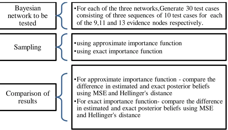
For experimentation, these networks are taken from the Genie and Smile [5]. The testing
of LLAIS will include comparing its sampling output (using approximate importance
function) with that from using exact importance function which is considered to be the
optimal one.
The comparison of performance using the exact importance function will help in knowing
how close the approximate importance function in LLAIS is able to reach the optimal
results. It is believed that computing the exact importance function will also affect the
running time of algorithm since it is the optimal and do not require updating and learning
of importance function as required by approximate importance function and hence saving
a lot of time.
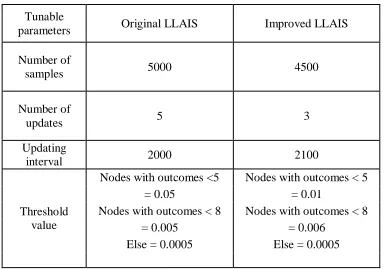
Further, there are various tunable parameters in LLAIS that will be discussed in chapter
4, we believe if the values of these tunable parameters are tuned properly it may lead to
the improvement in algorithm in terms of time efficiency and accuracy. Hence to
summarize the objective of this thesis is firstly, to test LLAIS algorithm for its scalability
and reliability by applying it on larger networks and secondly, tuning the various tunable
1.3 Overview of Thesis
The outline of the thesis is as follows:
Chapter 2: Background Study – In this chapter we will be giving a brief
introduction to the probability theory. Various concepts and notations will be concisely
discussed giving readers idea about the background of the probability theory. Section 2.2
discusses the probabilistic graphical models and why they are important to study. We will
also be giving gentle introduction to the Bayesian networks and inference in Bayesian
network including their mathematical and technical concepts. We will discuss major
exact and approximate inference techniques; focussing more on the approximate
inference in BN and hence discussing it in detail. This chapter will talk about the
multi-agent reasoning with MSBN and Linked Junction Forests (LJFs) and how inference is
done in LJF. Basically we tried to cover as much as possible the literature review of the
graphical models, BNs, MSBNs and reasoning in BN and MSBN, giving more emphasis
on the approximate algorithms for inference.
Chapter 3: Adaptive Importance Sampling in Bayesian Networks – This
chapter discusses the adaptive importance sampling applied in the context of Bayesian
networks and linked junction forests in MSBN. In this chapter we will be talking about
the algorithm LLAIS which is to be tested and explaining it in detail.
Chapter 4: Methods for testing and Improving LLAIS – This chapter
discusses the methods and experiments procedure followed in testing the scalability and
reliability of LLAIS. Further the improvement in LLAIS algorithm is also discussed by
Chapter 5: Testing and Improving LLAIS with Experiment Results – This
chapter discusses the experiment results of the testing of LLAIS on the larger networks.
The comparison of the results of LLAIS improved with original LLAIS will also be
discussed. On the whole this chapter include the graphs plotted for the experiments
results along with tables showing the information of comparisons made.
Chapter 6: Conclusion – This chapter includes the summarization of the thesis
with some directions for future research.
1.4 Thesis Contribution
As discussed so far the application of LLAIS is done on smaller network consisting of 37
nodes which is treated as local JT in LJF. LLAIS produced good estimates of local
posterior beliefs for this smaller network but its further application on larger networks is
not reported. So in this thesis, we tested LLAIS for its scalability and reliability on the
three larger networks treating them as local JTs in MSBN. It is important to test the
algorithm since the size of local JT can vary and go beyond 37 nodes network, on which
preliminary testing has been done. Our testing demonstrated that LLAIS is quite scalable
for the 56 and 76 nodes network but once it is applied to 109 nodes network its
performance deteriorates. The calculation of the exact importance function resulted in
saving a lot of time since it does not need updating and learning as required by the
approximate importance function, hence making the algorithm quite time efficient.
tuned properly it results in significant improvement in the performance of algorithm; the
improved LLAIS requires less number of samples and less updates than required by the
Chapter 2
Background Study
In this chapter, a brief introduction to the probabilistic graphs will be discussed, in
particular about the Bayesian network and Multiply Sectioned Bayesian network. The
inference including exact and approximate inference techniques will also be discussed.
2.1 Concepts in Probability
2.1.1 Probability Theory
The probability is the study of uncertainty. One of the most common notions of
probability theory is random variable. A random variable is a variable whose values are
outcome of a particular experiment. Just as the other variables random variables can take
any different values. From [1], all the possible outcomes of random variables are
mutually exclusive and collectively exhaustive. These outcomes together as a set form the
domain of the variables. The probability of a random variable is measured by a function
that maps each possible outcome, or instantiation, of this random variable into the
interval [0, 1].
Notations: Capital letters such as denote random variables. Bold capital
letters, such as X or Y, denote sets of variables and E usually denote the set of evidence
variables. Lower case letters, such as a and x denote particular instantiation of variable A
of sets X and Y respectively while the bold lower case letter e is used to denote the
observation for the set of variables E.
Given the set of random variables as * +, joint probability is defined as
a probabilities of all combinations of the possible outcome of each variable in .
Joint probability distribution or JPD is denoted as:
( ) ( )
( ),
where are the respective values which those variables may take.
The domain of is the cross join of the domains of all variables in * +;
further, each element from the domain of a set of variables is known as an instantiation of
these variables.
The Marginalization is defined as the process of summing out some variables from the
probability distribution. For example we can obtain the probability distribution of a
subset of by summing out all the variables in a set of excluding (which is
denoted as ).
Hence the Marginal Probability Distribution (MPD) of X from ( ) is denoted as :
( ) ∑ ( )
where ( ) is called the marginal probability distribution and can also be written as
It is to be noted that the probability distribution of some random variable is updated once
it observes the realization of another random variable or in other words we can say that
the probability distribution of random variables changes after receiving the information
that another variable has taken up some value. This is the relation of dependency and is
expressed as conditional probability distribution (CPD). Let and are two disjoint
subsets of , and let and be their instantiations (or values).
Then the CPD of given denoted as ( ) and also abbreviated as
( ) is formulated as:
( ) ( )
( ) (2.1)
where P( )
The conditional probability distribution of some variable with given evidence e, is
denoted as ( ) is also known as posterior probability distribution of
2.2 Probabilistic Graphical Models
The probabilistic graphical models provide ground to reason for uncertainties in real
world applications. These models use the knowledge given to them to make conclusions.
They play a key role in modeling uncertainties in the real world.
From [6] for example, sometimes a doctor might have to take information about the
patient- his name, symptoms, test results, personal characteristics to reach to the
conclusion what disease he might be suffering and what course of treatment has to be
affected by many factors, it is because due to large systems we are often not sure about
the true state of the system. It may be due to the fact that our observation is partial or it
may be due to that only some aspect of the world is being exposed to us. As a result, it
might happen that true disease of the patient is not observed directly or even the future
prognosis made by him is never observed. Further it has to be kept in mind that due to
lack of observation we are not clear about the true state of world, so we can say that
relationships are not deterministic; hence it can happen that there are very few diseases
where we can have true relationship between the disease and its symptoms and even
fewer such relationships between the disease and its prognosis. So there was a need for
reasoning system to take into account all the different possibilities about the state of
world.
The probability theory provides us with the formal framework where multiple possible
outcomes and their likelihood can be considered. So the probabilistic framework helped
in deterministic specification of the behavior of the complex system
The probabilistic graphical models are significant tool in helping the agent to reason
about its uncertain domain and taking the action accordingly. These models use graphical
representation to represent the complex probabilistic distribution. The graphical models
are described [7] as representation of probabilistic structure along with functions that are
used to derive the joint distribution. From [1], the probabilistic graphical models merge
graph theory where the data is modeled as a set of nodes which represent random
variables and the connecting arcs represent the dependencies between the variables.
2.3 Dependency Model
The probabilistic model for a set of random variables is defined by joint probability
distribution but in order to specify a probability model using full JPD is an impractical
task. Since the domain described by boolean variables requires a table of size ( )
and takes ( ) time to process that table, so to lower down this cost we have to take
into account the advantages of dependence and independence relationship among
variables.
Let be disjoint subsets of
and are unconditionally independent if the following conditions will hold:
( ) ( ) ( ) (2.2)
The above unconditional independency can be denoted as conditional independency
statement (CIS) ( )or ( ).
and are conditionally independent given if the following holds:
( ) ( ) ( ) (2.3)
The above conditional independency relation can be expressed as conditional
independency statement (CIS) I(X, Z, Y) or I(X, Y|Z).
We can conclude that dependency model is any model M of a set of variables denoted
as * +, from where we can decide whether I(X,Y|Z) is true or not
An easy and direct way to model dependency models is to use directed acyclic graphs
(DAG). DAG stands for directed acyclic graph consist of set of nodes as the random
variables, and a set of directed links between nodes but with no directed cycles. The
Bayesian network is represented in the form of DAG. To identify the independency
relationship in DAG, concept called d-separation is used.
Definition 2.1: D-separation
Let be a Directed Acyclic Graph and be disjoint set of nodes in . A path
between nodes and is closed by if one of the following two conditions
holds: (1) There exists that is either tail-to-tail or head-to-tail on There exists a
node that is head-to-head on and neither or any descendant of is in . If both
conditions fail, then is rendered open by .
Nodes and are d-separated by if every path between and is closed by ;
and are d-separated by if for every and , and are d-separated by
2.4 Bayesian Network - Definition and Example
The Bayesian networks have been seen as a powerful tool in Artificial Intelligence in
order to simulate and approximate real situations. They are defined as probabilistic
graphical model for reasoning under uncertainty [1]. It provides the coherent framework
for the various decision support systems which function using uncertain knowledge
available to them, such as in machine learning, bioinformatics, medical diagnosis and so
In [7], Bayesian networks also known as belief networks, causal probabilistic networks,
directed Markov fields or influence diagrams (given some additional structure). It is a
directed acyclic graph in which nodes represent random variables, and arcs represent
direct probabilistic dependence between directly connecting variables. Each node is
assigned probabilistic distribution conditioned on that node‟s parents. Then Joint
probability distribution determined from the factorization of CPD‟s assigned.
From [8], Bayesian Network is a triplet ( ) is a set of variables, is a
connected DAG whose nodes correspond to one-to-one to members of such that each
variable is conditionally independent of its non-descendants given its parents. Each
variable in is represented as a node in DAG, it is associated with CPD denoted by
which is defined as:
* ( ( )) +
Here the ( ) denote the parents of node in the DAG. The product of these CPD‟s
defines JPD given as:
( ) ∏ ( | ( ))
(2.4)
Equation 2.4 defines the factorization which is also known as Bayesian factorization
done in terms of CPDs. The DAG is commonly referred to as dependency structure of
Bayesian network.
Hence we conclude that Bayesian network models by providing the compact
representation of JPD also captures the independency among random variable.
Figure 2.1: The Asia Travel Network-simple BN.
The Asia Travel Bayesian network is DAG defined over the set of variables
where * +,
the corresponding set of CPDs is:
* ( ) ( ) ( ) ( ) ( ) ( ) ( ) ( )+,
These two components will now define Joint Probability distribution (JPD) and expressed
as:
( ) ( ) ( ) ( ) ( ) ( ) ( ) ( ) ( ), (2.5)
the CPD factorization in above Equation 2.5 gives the Bayesian factorization of ( )
2.5 Inference in Bayesian Networks
The assignment of values to the observed variables is known as evidence. The most
important form of reasoning used in Bayesian networks is called belief updating which
the value of their evidence is given. A lot of research is being done in the field of
reasoning. In [9], the Bayesian network is known to provide the efficient and natural way
for modeling the causal structures along with the computational basis for probabilistic
inference. The inference task in the Bayesian network is represented as ( )
where denotes the set of variables and denotes evidence set; while set of variables
is denoted as hidden variables and is represented by . Since we have joint
probability distribution defined over the random variables so probabilistic inference can
be performed by summing out the hidden variables using the sequence of multiply and
addition operations.
2.5.1 Exact Inference
The calculation of exact value of posterior probability is called exact inference.
The following Equation 2.6 calculates for the exact value for inference according to the
probability theory [1]:
( )
( )( ) = ( ) ∑ ( ) (2.6)
where is a normalization value ( ).
So, in order to calculate the value of ( ), we need to perform summation over all
variables except for the evidence variables in ( ) There are different ways to
process summation giving rise to different algorithms, only idea behind them is getting
the value of evidence using minimum number of computations. It is a combinatorial
optimization problem [7]. The Enumeration algorithm for computing the posterior
operations involved. So, many have been developed to make the inference approachable
and easy.
As asserted in [10], In 1980s, Pearl gave the algorithm for efficient message passing for
inference for polytrees but it was regarded as polynomial time complexity in number of
nodes, later he gave exact inference algorithm for multiply connected networks called
loop cutset conditioning. The loop cutset conditioning algorithm works by changing the
connectivity of the multiply connected graph rendering it singly connected graph and
instantiating the selected subset of nodes that are referred as loop cutset. The complexity
for this algorithm is calculated from the number of different instantiations that need to be
considered and resulting in its time complexity growing exponentially with the size of
loop cutset being ( ), where d is the number of values which random variables can
take and c giving the size of loop cutset so here it is required to reduce the size of loop
cutset in case of multiply connected networks but the problem of finding the minimum
loop cutset is known to be NP-hard.
The variable elimination (VE) algorithm works by eliminating variables other than the
queries one by one by summing out them. The complexity of VE can be measured by the
number of numerical multiplications and numerical summations it performs. An optimal
elimination ordering is one that results in the least complexity. The problem of finding an
optimal elimination ordering is NP-complete.
by Lauritzen and Spiegelhalter [11]. The inference task is performed on secondary
structure of BN which is junction tree. A junction tree (JT) is a graph which is formed by
the nodes that are subsets of the domain variables called clusters or cliques.
The following steps will elaborate in detail about the conversion of Bayesian network to
the junction tree:
Step 1. Moralizing the original graph: Moral graph is formed by connecting the pair of
nodes that have common child, that is, two nodes with same child are said to be married,
and then replacing the directed edges with undirected edges.
Step 2. Triangulating the moral graph: In a triangulated graph, for every cycle of length
greater than or equal to four, a link is drawn between two non-adjacent nodes on the
cycle. The problem for finding the optimal triangulation is NP-complete [12], but fast
triangulation algorithms that can produce high quality results are available [13] [14].
Step 3. Identifying the cliques: After the triangulation has been performed we identify the
cliques. A clique or cluster is nothing but a maximal complete subgraph. Every clique
corresponds to the node of junction tree.
The JT is constructed using an important property which is called running intersection
property [1] which says that if a variable belong to two distinct JT clusters, then it should
belong to every cluster on the path connecting the two clusters. So taking this property as
the basis the set of common nodes to a pair of neighboring clusters are defined as their
Separators. The construction of optimal JT is discussed in [15]. Once the junction tree is
It is product of all the conditional probability distributions which the clique has received.
If a clique has not received any CPD it will be initialized to 1. The initial potential of the
cluster does not represent cluster marginal so message passing has to be done so that the
information of probability distribution of each cluster is made consistent to the other
clusters.
The Hugin architecture [16] [17] and the Shenoy-Shafer architecture [18][19][20] are the
two major variations for the JT-based exact inference calculations. The clique tree
propagation works well with sparse networks but its performance gets affected as the size
of network increases. Its complexity is exponential to the size of the largest clique made
out from the undirected graph.
But unfortunately the problem of exact inference in Bayesian networks is NP-hard. So as
the researchers were faced with intractability of exact inference in large and complex
networks, so it led them to investigate to develop the approximate inference algorithms as
an alternative.
2.5.2 Approximate Inference
Today when the size of practical models is increasing to the size of hundreds of variables,
the problem of finding the feasibility of probabilistic inference becomes important. The
exact inference algorithms including the JT algorithm become impractical and [7] when
applied to larger and complex networks it require either prohibitive amount of memory or
Although the approximation algorithm to the desired precision is also shown to be
NP-hard [21] but they are the only alternative which can produce any result at all.
As discussed in [1] [7], the various approximate inference techniques developed so far
are:
Model Simplification: This method simplify the original structure of model in some way
and hence weakening the network dependencies and then exact methods can be applied to
the simplified network so as to obtain the approximation solution. These simplification
methods involve the reduction in the cardinality of the size of JT clusters [22], some
methods reduce the model complexity by annihilating small probabilities [10], Sarkar‟s
algorithm approximates the Bayesian network by finding the optimal tree-decomposable
representation which is closest to the actual network. Another most widely used method
is reducing the edges of an original network. Some simplification methods also involve
using the variational methods for fitting parameters to simple logistic function [23] [10].
Search Based Algorithms: Search based methods assumes that small fraction of joint
probability mass contain the majority of probability mass. It finds the high probability
instantiations with large probability mass in the joint probability distribution and uses
them to obtain reasonable approximations. These methods give good approximations of
the network with almost all extreme conditional probabilities. These include Henrion‟s
“Top-N” search based methods [24], Poole‟s search approach using conflicts [25] [26]
Loopy Belief Propagation: As discussed in [28], there has been a lot of research going
on the use of Pearl‟s polytree propagation in Bayesian network with loops. In [29]
researchers have analytically demonstrated that loopy belief algorithm can perform quite
well in error-correcting codes and computer vision. It performs well on the graphs with
loops but fail to give good convergence when the density of graph increases resulting in
poor results.
Stochastic Sampling Methods: The stochastic sampling algorithms also known as
Monte-Carlo algorithms are the most well- known and most commonly used simulation
methods. These algorithms generate randomly selected instantiations of the network as
per the probabilistic distributions of the model and then the frequencies of these
instantiations are calculated for nodes of interest as an approximation of the inference.
The accuracy of these algorithms depends upon the size of samples irrespective of the
topology of the network. The most important characteristic of the stochastic sampling
algorithm is its nice any-time property such that the computation can be interrupted at
any given time in order to yield an approximation [10].
The main idea behind the stochastic sampling algorithm which is the class of algorithm
under approximate inference is that these algorithms sample the probability distribution
and estimate the probability of queries depending upon the samples obtained by
calculating the frequencies of instantiations of interest. The advantage of using the
stochastic sampling is that the execution time is independent of the topology of network
such that their computation can be interrupted at any time with guaranteed results [7].
2.6 Sampling in BN
The sampling algorithms are the most common approximate inference technique used for
calculating the posterior probabilities. The main idea behind the sampling is to randomly
instantiate each node in Bayesian network in topological order and produce single
sample. These samples are generated a number of times and finally after some specific
number of times or after generating some specific amount of samples the posterior
probabilities are calculated for each node by counting the frequency of each possible
instantiation of every node in all the samples generated. Now we will discuss some of the
common sampling algorithms:
1. Forward Sampling: It is the simplest sampling algorithm. In this we start by
ordering the nodes in topological order, assign the values of evidence variables and
number of samples generated. The sampling will proceed by first sampling the parent
node and then the child node. The evidence nodes are instantiated to observed state and
so omitted from sample generation. The root node is randomly instantiated to one of its
possible states as per the prior probability of this node and child node is instantiated
depending upon the parent node instantiation, to one of its possible states according to the
conditional probability distribution. The procedure is followed a number of times, once
samples are generated, the posterior probability ( ) is obtained calculating the ratio
2. Likelihood Weighting: The LW sampling is same to the forward sampling but it
never discards the sample [43] [44]. It assigns weight to each sample generated. Suppose
we have Bayesian Network which has evidence nodes as that are
instantiated to respectively. Then the weight of the sample will be
calculated as ( | ( )) ( | ( )) ( | ( )).
In other words the weight of the sample is the product of the probability that each
evidence node will have the desired value given the value of its parents in the sample .
Once number of samples are generated the posterior probability is calculated for each
node and each possible value by summing out weight of sample in which is
instantiated to and divided by total weight of all samples.
It is most commonly used simulation method for Bayesian network inference. It is simple
and is able to increase the precision by generating more number of samples than the other
algorithms in the same amount of time. Its convergence deteriorates when the evidence is
very unlikely.
3. Importance Sampling: Importance sampling is same as the generic sampling
algorithm [44]. The importance sampling has two variants called self-importance (SIS)
and heuristic importance. Here the importance function is updated trying to revise the
conditional probability tables periodically in order to make the sampling distribution
gradually approach the posterior distribution. From [45], since the data used to update the
importance function and to compute the estimator, this process introduces bias in the
heuristic importance [44] [46] but promising direction in the work on sampling
algorithms has not been achieved yet. Now, we will be going through the theoretical roots
of importance sampling since it is the basic step to understand in order to learn about the
existing know-how of stochastic sampling algorithms for Bayesian networks which will
ground the basis of our thesis.
2.6.1 Mathematical Foundation of Importance Sampling
Let ( ) be the function of variables ( ) over a domain
such that computing ( ) for any is feasible. Consider the problem of approximate
computation of the integral
∫ ( ) (2.7)
Importance sampling approaches this problem by writing the integral (2.7) as
∫ ( ) ( ) ( ) (2.8)
where ( ) often called importance function, is a probability density function over Ω.
The samples can be generated from ( ) using importance sampling if the importance
function is zero only when the original function is zero, that is, ( ) ( )
Once the samples have been generated from n points as according
to the probability density function ( ), we can estimate the integral I by
̂
∑
( )( )
(2.9)
̂
( ̂
)
( )
∑
(
( )
( )
̂
)
(2.10)
The estimator thus obtained has the following properties:
1. ( ̂ )
2. ̂
3. √ ( ̂ ) → ( ( ))
( ) ∫ ( ( )
( ) ) ( )
4.
. ̂
( ̂
)/ ̂
( ̂
)
( )The variance ̂ is proportional to ( ) and inversely proportional to the number of
samples. To minimize the variance we can either increase the number of samples or we
can reduce ( ). Taking into consideration latter, [47] reports the following theorem and
corollary:
Theorem 2.6.1: The minimum of ( )is equal to
( ) (∫ ( ) )
And occurs when is distributed according to the following probability density function
( ) ( ) ∫ ( )
Corollary 2.6.1: If ( ) , then the optimal probability density function is
( ) ( )
In practice, sampling precisely from ( ) ( ) will happen very rarely but we still
expect that the functions close to it can help in reducing the variance effectively. Usually
the closer the shape of the function ( ) is to the shape of the function ( ), the smaller
is ( ) It is essential to put in more strength towards choosing the importance function
whose shape is as close as possible to that of ( ) than to apply the Brute-force method
of increasing the number of samples.
It is worth noting that when ( ) is uniform then the importance sampling becomes
general Monte-Caro sampling. One another property of importance sampling is that one
should avoid ( ) ( ) ( ) in any domain of sampling even if ( ) matches
well with ( ) , it is because in this case the variance can become very large or even
infinite. In order to adjust this we can make ( ) to be larger in unimportant regions of
the domain of
Till now we discussed about the importance sampling for continuous variables but the
results discussed remains valid for discrete variables where the integration is substituted
with summation.
2.6.2 Importance Sampling for BN
From [1], the family of stochastic sampling belongs to the BN approximate algorithm
class. The importance sampling is commonly used simulation technique which is used to
approximate the average over a set of numbers by an average over a set of sampled
numbers.
In order to evaluate the sum ∑ ( ) for some real function , samples are
generated from the importance function such that ( ) ( ) , we have
∑
( )
∑
( )( )
( )
0
( ) ( )1 (2.11)
By the definition of expected value we can estimate I as
̂
∑
(
)
(2.12)
where (
)
( )( )
,
is called sample weight or score.In order to compute the probability of evidence ( ) from a JPD ( )
∏ ( ( )) of a BN model, we have to sum over all the non-evidence nodes:
( ) ∑ ( ) (2.13)
= ∑ ∏ ( ( ) )
Let , we simplify the above equation 2.13 as:
( ) ∑ ( ) (2.14)
We can apply the principal of importance sampling.
Assume that our proposal distribution or sampling distribution Q is the importance
function such that ( ) ( ) .
Equation 2.14 can be re-written as:
(E ) ∑ ( )
( )
( )
By the definition of expected value, we have
∑ ( )
Equation 2.15 becomes:
( )
0
( )( )
1
, ( )-
(2.16)where ( ) denote the score of each sample and is calculated as:
( ) ( ) ( )
Suppose we sampled from Q and obtained a sample set ( ) then
̂( )
∑
( )( )
∑
(
)
(2.17)As the size of sample increases the expected value will approach the true average. It
means we can say that as ̂( ) ( ), thus such estimator is
unbiased.
In order to obtain the posterior probability ( ) we can separately compute the two
terms ( ) and ( ) and then combine them by the definition of conditional
probability.
̂(
)
̂( )̂( )
∑ ( ) ( )
∑ ( )
(2.18)
where ( ) if and only if the sample contains , Otherwise ( )
It is important to note here that two terms ( ) and ( ) can be
separately estimated unbiasedly, the estimation thus obtained by combining them through
Equation 2.18 is not an unbiased estimator [45].
The quality of importance function depends upon how close the sampling distribution is
to the true distribution. Many importance sampling algorithms have been developed so
far for Bayesian networks where choice of importance function may vary from the prior
distribution as in the likelihood weighting algorithm [6] to more refined choices such as
there exist algorithms that update the importance function through learning processes [45]
or calculate the importance function directly with loopy belief propagation [48].
The main aim of these methods is to ultimately reach the optimal importance function,
which is a function proportional to the posterior distribution and should have a thick tail
[49] [50]. This section has discussed in detail about the mathematical foundation of
importance sampling and how it is applied in context of Bayesian networks for
approximate reasoning.
2.7 Multiply Sectioned Bayesian Network (MSBN)
Today intelligent systems are being applied to the larger and complex domains and there
are many applications that are found to be suitably addressed by multi-agent systems [30]
[31]. In [6], multi-agent system is the one which consist of a number of agents interacting
infrastructure. In general cases, the agents will be acting or representing users or owners
having different goals and motivations.
The problem domain in multi-agent systems is distributed naturally among the agents and
typically with increased size and complexity, so in order to model such a domain as
single BN becomes difficult and performing inference becomes challenging [8]. As a
result it is natural to consider one single, large and complex domain being divided into
subdomains; where each subdomain is individually represented and managed by a
relatively light weighted single agent. The basic assumption taken is that these agents are
expected to be cooperative in the sense that they will always provide truthful information
about their local domains to other agents.
The Multiply Sectioned Bayesian Network (MSBN) [8] extends the traditional BN model
from a single agent oriented paradigm to the distributed multi-agent paradigm and
provides a framework to apply probabilistic inference in distributed multi-agent systems.
Under MSBNs, a large domain can be modeled modularly and the inference task can be
performed in coherent and distributed fashion.
The MSBN model is based on the following five assumptions:
1. Agent‟s belief is represented as probability.
2. Agents communicate their beliefs based on a small set of shared variables.
3. A simpler agent organization is preferred.
5. An agent‟s local JPD admits the agent‟s belief of its local variables and
the shared variables with other agents.
An MSBN [32] consist of inter-related Bayesian subnets and each subnet encodes agent‟s
knowledge on a subdomain. The agents are organized in hypertree structure and
exchange of messages is done through hyperlink between the adjacent agents. The
complexity of communication among all the agents is linear on the number of agents and
the complexity of local inference is the same as if subnet is a single agent based Bayesian
network.
The MSBN is described in terms of the following definitions [8].
Definition2.2: Let ( ) be a connected graph, with the set of random variables V
and connecting edges E, sectioned into subgraphs * ( )+
Let the subgraphs be organized into an undirected tree where each node is uniquely
labeled by a and each link between and is labeled by the non-empty interface
such that for each is contained in each subgraph on the path
between in ψ. Then ψ is a hypertree over G. Each is a hypernode and each
interface is a hyperlink.
Definition 2.3: Let G be a directed graph such that a hypertree over G exists. A node
contained in more than one subgraph with its parents ( ) in G is a d-sepnode if there
exists at least one subgraph that contains ( ). An interface I is a d-sepset if every
Definition 2.4: A hypertree MSDAG where each is a DAG, is a connected
DAG such that (1) there exists a hypertree ψ over G, and (2) each hyperlink in ψ is a
d-sepset.
Definition 2.5: An MSBN M is a triplet (V, G,P). is the domain where each
is a set of variables. (a hypertree MSDAG) is the structure in which nodes of
each DAG are labeled by elements of . Let be a variable and ( ) be all the
parents of in G. For each , exactly one of its occurrences (in a containing (* +
* +) is assigned ( | ( )) and each occurrence in other DAGs is assigned a
uniform potential. ∏ is the JPD, where each is the product of the potentials
associated with nodes in . A triplet ( ) is called a subnet of M. Two
subnets are said to be adjacent if are adjacent on the hypertree
MSDAG.
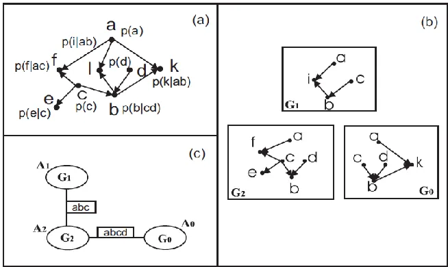
Figure 2.2 below shows an example [2] where subnets in an MSBN are satisfying the
hyper tree condition. Here (hence the hypertree condition is trivially
satisfied). But in general can be non-empty. The interface between the subnets in
an MSBN must form a d-sepset. So here each of the in the interfaces is a
d-sepnodes. Hence, the interfaces * + and * + are d-sepsets. If we reverse the arcs
from j to l, the node j would no longer be a d-sepnode consequently * + would no
longer be a d-sepset. Both the hypertree and d-sepset conditions ensure syntactically that
Figure 2.2: The Graph G in (a) is sectioned into and in (b). ψ in (c) is a hypertree over G.
An MSBN consists of a set of inter-related Bayesian subnets, each of the subnets
encoding the agent‟s knowledge on the subdomain. Every agent maintains its local BN
subnet which represents the partial view of the entire larger problem domain. The union
of all subnet DAGs must be a DAG and these subnets are organized into hypertree
structure. Each node in hypertree corresponds to the subnet and each hyperlink
corresponds to d-sepset, which are the shared variables between the adjacent subnets. The
hyperlink renders the two sides of the network conditionally independent. MSBN
provides a framework for uncertainty reasoning in cooperative multi-agent systems.
Today MSBN have been used in many fields such as building surveillance [33], medical
and equipment diagnosis [34][35]. MSBN have also been used to provide support for the
object-oriented Bayesian networks [36].
2.8 Linked Junction Tree Forests (LJFs) in MSBNs
called linked junction tree forest (LJF). We can say that LJF is derived dependence
structure which is adopted for distributed probabilistic inference in MSBNs. An LJF [37]
is constructed through the process of cooperative and distributed compilation so that each
hypernode in hypertree is transformed into a local JT and each hyperlink into a linkage
tree. A linkage tree is nothing but it is a special name given to the junction tree
constructed from a d-sepset. In a linkage tree, each cluster is called a linkage and each
separator is known as linkage separator. The cluster in the local JT which contains a
linkage is called Linkage host. The two adjacent subnets maintain their own linkage tree
corresponding to the same d-sepset.
The Linked Junction Forest LJF as described in [8]:
Definition 2.6: A linked Junction Forest is a tuple (V,G,T,L)
is the total universe where each is a set of variables called a subdomain,
, where each ( ) is a chordal graph such that there exist a hypertree
ψ over G.
* + is a set of JTs, each of which is a corresponding JT of .
* + is a collection of linkage tree sets. Each * + is a set of linkage trees, one
for each hyperlink incident to in ψ. Each is a linkage tree of with respect to a
hyperlink .
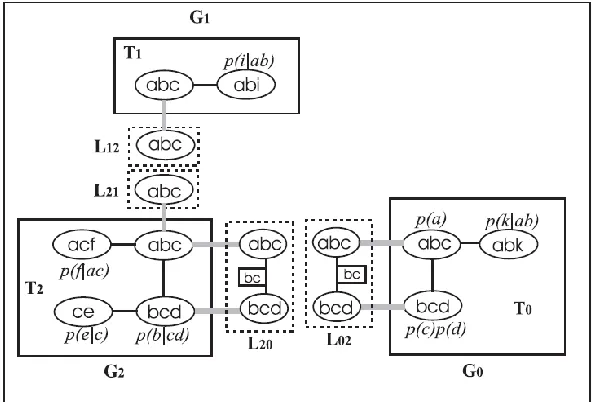
Figure 2.3 shows the Bayesian network which is sectioned into three subnets and its
corresponding MSBN hypertree structure. The three subnets being formed are
tree structure is formed, it is converted to the LJF and inference is carried out in this LJF
structure which is secondary structure of MSBN. Figure 2.4 shows the LJF constructed
from the MSBN in Figure 2.3. Here the local Junction trees are are
constructed from the BN subnets respectively, shown in the solid line
boxes. The linkage trees are derived from the d-sepsets and enclosed in dotted line boxes.
Each pair of adjacent subnets maintains identical linkage trees. For example, the linkage
tree contains the linkage and and their linkage hosts in are the clusters
* + and * +.
Figure 2.3: (a) A BN (b) A small MSBN with three subnets (c) the corresponding MSBN hypertree.
2.8.1 Initialization of LJF
During the initialization process of LJF, [37] exactly one of all the occurrences of a
variable (from the subnet containing * + * +) is assigned the CPD ( | ( ))
and all other occurrences are assigned unity potential. Along with it unity potential is also


![Figure 5.2: [5] Structure of Hailfinder Bayesian network](https://thumb-us.123doks.com/thumbv2/123dok_us/1416720.1174216/81.612.183.429.243.468/figure-structure-hailfinder-bayesian-network.webp)
![Figure 5.9 : [5] Structure of win95pts Bayesian network](https://thumb-us.123doks.com/thumbv2/123dok_us/1416720.1174216/89.612.177.435.156.408/figure-structure-win-pts-bayesian-network.webp)