DEVELOPMENT OF CONDENSATION MODEL AND
IMPLEMENTATION IN CFD CODE FOR HYDROGEN DISTRIBUTION
CALCULATIONS
R. Srinivasa Rao1, Teany Thomas2, Kannan N Iyer2, S. K. Gupta1
1
Safety Analysis and Documentation Division, Atomic Energy Regulatory Board, Mumbai, INDIA- 400094
2
Mechanical Engineering Department, Indian Institute of Technology, Mumbai, INDIA E-mail of corresponding author: [email protected]
ABSTRACT
Large amount of hydrogen could be generated and released into the containment building during accident conditions in a nuclear power plant. The integrity of containment could be challenged by certain hydrogen combustion modes. As boundaries between the different combustion modes are characterized by narrow gas concentration bandwidths, accurate gas distribution calculations are needed. This is one of the more important safety issues that are being currently addressed. In spite of extensive research in this area there is still a need to reduce uncertainties concerning some important phenomena. One of these is transport and distribution of hydrogen in the reactor containment in the presence of steam. Analysis using a multi-dimensional computational tool, such as Computational Fluid Dynamics (CFD) code is necessary to predict the local behaviour. However, the commercial CFD codes do not have built in condensation models. These models have to be implemented and validated before applying it to containment distribution calculations.
As detailed knowledge of containment thermal hydraulics is necessary to predict the local distribution of hydrogen, steam and air inside the containment, considerable efforts have been undertaken internationally to understand the associated phenomena by conducting a large number of experiments and then subjecting the test results to extensive analytical assessment. To develop an understanding of thermal hydraulic behaviour in Indian power reactor containments, a program has been undertaken. In this direction a condensation model was developed in line with international developments and implemented in the CFD code FLUENT through user defined functions. The user defined functions for sinks of mass, momentum, energy, and species balance equations together with associated turbulence quantities viz., kinetic energy and dissipation rate have been developed. After implementation of this model in CFD code through user defined functions, the model was benchmarked for a simple flow domain (idealized version of the CONAN test facility) against the correlation based on analogy between heat and mass transfer and the predictions reported in the literature.
INTRODUCTION
Significant amount of hydrogen could be generated due to metal water reaction and released into the containment during the accident conditions in a nuclear power plant. This may result in local hydrogen concentration sufficient to pose a threat of hydrogen deflagration or detonation. Such events could increase the containment pressure, which could affect the containment integrity. As boundaries between the different combustion modes are characterized by narrow gas concentration bandwidths, sufficiently accurate gas distribution predictions are needed. Detailed knowledge of containment thermal hydraulics is necessary to predict the local distribution of hydrogen, steam and air inside the containment. Multi-dimensional computational tool, such as Computational Fluid Dynamics (CFD) code, is necessary for accurate prediction of hydrogen distribution. However, the commercial CFD codes do not have all the required models for prediction of hydrogen distribution and need to be incorporated. The condensation model is one such model to be incorporated. In this direction, a condensation model was implemented in the CFD code, FLUENT through user defined functions. This model was benchmarked against the idealized version of the CONAN test facility.
DEVELOPMENT OF CONDENSATION MODEL
Fig. 1: Film condensation with non-condensable gases on a wall
The condensation model incorporated in CFD code FLUENT through user defined functions (UDFs) is similar to NRG model [1]. The convective flow of gas occurs due to steam condensation at the wall. The mass balance of steam at the interface (subscript i) between gas and condensate film at the wall is:
Condensation flux = Steam transported through bulk motion + Diffusive transport
If the condensation flux at the wall is ni, consequently, the bulk motion of the gas to the interface is equal to
ni as the film is impervious to non-condensable. In general, in a multi-component diffusion-convection the total flux
consists of diffusion flux and convection flux. The diffusion flux near the wall can be represented through a mass transfer coefficient, gm. The total flux of any species can then be represented by ݊ݔ+ ݃(ݔ − ݔ), where x and xi
are the species mass fraction at the wall adjacent cell and at the wall respectively. The mass transfer co-efficient is a function of turbulence near the wall and is usually calculated by a CFD code internally. In the present case, as on the wall the total mass flux is the condensation flux, we can write:
݊= ݊ݔ+ ݃(ݔ − ݔ) (1)
The above equation can be reformatted as: ݊=(௫ି௫)
(ଵି௫) (2)
Numerically, this can be expressed as: ݊=(௫ି௫ೢೌ)
(ଵି௫ೢೌ) (3)
Where, x = steam mass fraction
xi = steam mass fraction at the interface
The mass fraction xwall of steam at the surface of the condensate film at the wall is calculated from the
vapour pressure at the surface. The Antoine equation is used to describe the vapour pressures as a function of the surface temperature:
൬
ೝ(ೌ)൰ = ܣ +
்ା (4)
The co-efficients A = 23.1512, B = -3788.02 K and C = -47.3018 K are fitted for the data obtained from steam tables. The mass of the steam that condenses has to be removed through a mass sink at the wall. The associated enthalpy sink is required to remove the enthalpy associated with the mass of steam condensed. It is assumed that the condensing wall immediately removes the condensation heat. The enthalpy sink Q for each cell is calculated by:
ܳ = ݊ܣ௪ܥ൫ܶ− ܶ൯
(5)
Tref is the reference temperature at which the enthalpy is zero. The turbulent quantities associated with thismass are also to be removed. The sinks of the turbulent quantities are calculated by: Condensate
film
Temperature
profile
Gaseous
boundary layer
Steam
concentration
profile
T
∞T
ITurbulent kinetic energy (k) sink is given by:
ܵ = ݊ܣ௪݇ (6)
Turbulent energy dissipation rate (ε) sink is given by:
ܵఌ = ݊ܣ௪ߝ (7)
These mass, energy, turbulent quantities such as kinetic energy and energy dissipation rate and species sink (steam sink) are modeled using UDFs and implemented in the CFD code FLUENT.
BENCHMARKING OF THE CONDENSATION MODEL
The benchmark exercise involves simulation of the condensation in a flow domain representing channel type geometry. The aim of this exercise was to compare with the correlation based on heat and mass transfer analogy for a classical problem of condensation on a flat plate.
ܵℎ௫ = 0.0296 ܴ݁௫.଼ܵܿ.ଷଷ (8)
The University of Pisa proposed an initial step of the Benchmark (identified as the 0th Step) aimed at comparing code responses among each other and with applicable correlations in the application to a classical problem of condensation on a flat plate. The reference geometrical and operating conditions for this step were selected as an idealization of the CONAN experimental facility operated at the University of Pisa [2].
Problem Description
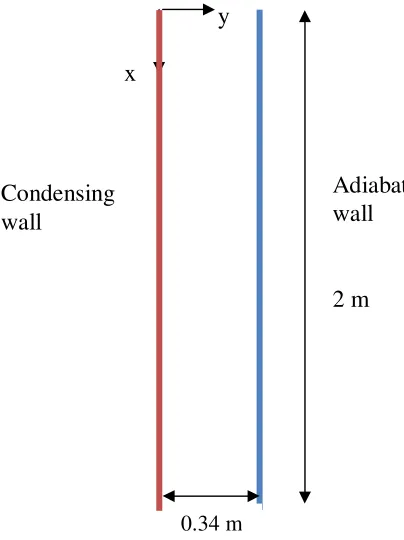
The geometrical configuration of the problem considered is shown in Figure 2. The geometrical configuration of the problem is an idealized version of the CONAN test facility. A channel of 0.34 x 2.0 m is considered as a flow domain for this exercise. Table 1 indicates the initial and boundary conditions specified for inlet velocity, mass fractions and wall temperatures. Four heat and mass transfer cases were analysed with two different velocities and wall temperatures. The values of inlet velocity were selected in order to allow the analysis of computed data at sufficiently large Reynolds numbers, to assure that the forced convection correlations are applicable at least in the last part of the channel. The heat and mass transfer cases involved a saturated air and steam mixture at the assigned inlet temperature. The right wall is adiabatic wall where heat flux is zero.
Fig. 2: Geometrical configuration
The thermal conductivity and specific heat at constant pressure are assumed to be constant throughout the calculation. Density is computed from incompressible ideal gas law and viscosity is computed from the mixing law.
y
Condensing
wall
Adiabatic
wall
2 m
x
For the present analysis, the Fickian diffusion approach is used. Diffusion coefficients used are obtained from the handbook of Vargaftik et al. (1975) [3]. The diffusion co-efficient of steam is obtained from air-steam system and a value of 0.3451 cm2/s is used and kept constant throughout the calculation. The turbulence model k-ε is used. Near wall modelling is treated using enhanced wall treatment to resolve the viscous sub-layer.
The turbulence model k-ε is used for benchmarking of this problem. Near wall modelling is treated using enhanced wall treatment to resolve the viscous sub-layer. Enhanced wall treatment is a near-wall modeling method that combines a two-layer model with enhanced wall functions. If the near-wall mesh is fine enough to be able to resolve the laminar sub-layer, then the enhanced wall treatment will be identical to the traditional two-layer zonal model.
Table 1: Initial and boundary conditions for both pure heat transfer and heat and mass transfer Test name Inlet velocity
(m/s)
Twall (K) Tinlet (K) Inlet vapour
mass fraction
P (Pa)
HMT-30-3 3 303.15 363.15 Saturation 101325
HMT-30-6 6 303.15 363.15 Saturation 101325
HMT-60-3 3 333.15 363.15 Saturation 101325
HMT-60-6 6 333.15 363.15 Saturation 101325
Grid Sensitivity Study
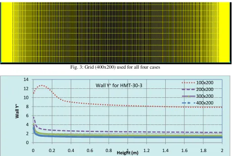
The grid sensitivity calculations are performed with different grid sizes of 100x200, 200x200, 300x200 and 400x200. The cut view of the 400x200 grid is shown in Figure 3. The wall y+ values for the left wall for these grid sizes are shown in Figure 4. The option last to first ratio of 10 was used to refine the grid at the walls except for 100x200 grid. However, the successive ratio option was used to refine the grid at the wall for 100x200 grid. The wall y+ values for the left side wall are in the range of 8 to 10 for the grid 100x200 and 2 to 3 for the grid 200x 200 except in the inlet region. The wall y+ values for the left wall are in the range of 1.5 to 2 for both the grids 300x200 and 400x200 except in the inlet region.
Fig. 3: Grid (400x200) used for all four cases
Fig. 4: The wall y+ values for different grids 0
2 4 6 8 10 12 14
0 0.2 0.4 0.6 0.8 1 1.2 1.4 1.6 1.8 2
W
a
ll
Y
+
Height (m)
100x200 200x200 300x200 400x200
The grid sensitivity calculations are performed with different grid sizes of 100x200, 200x200, 300x200 and 400x200 and results of which are shown in Figure 5 for the case HMT-30-3. The sensitivity of the predictions with the grid sizes of 100x200 and 200x 200 is quite significant. However, the results show less sensitivity for the grid sizes beyond 300x200 and 400x200. Therefore, the grid size of 400x200 was selected for benchmarking of this problem for all the four cases viz. HMT-30-3, HMT-60-3, HMT-30-6 and HMT-60-6. The expressions or computations of Sherwood number (Sh), Schmidt number (Sc) and local Reynolds number (Rex) are described in the subsequent sections.
Fig. 5: Grid sensitivity on the results
Results and Discussion
As discussed above four cases with two different wall temperatures and two different inlet velocities are analysed. This section deals with the predictions of these cases.
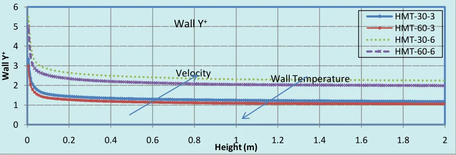
Assessment of y+values
The following figure (Figure 6) shows the wall y+ (u*y/ν ) values obtained for the all four cases viz. HMT-30-3, HMT-30-6, HMT-60-3 and HMT-60-6. The grid size of 400x200 is used for all the four cases. The wall y+ values are in the range of 1 o 1.5 for the cases with inlet velocity of 3 m/s (HMT-30-3 and HMT-60-3) except in the inlet region. Whereas, the wall y+ values are in the range of 2 to 2.5 for the cases with inlet velocity of 6 m/s (HMT-30-6 and HMT-60-6) for the entire wall region except in the inlet region. Ideally, the y+ value should be around 1. However, up to a value of 5 can be used. Because all these values are less than 5, the near wall mesh resolution is in the laminar sub-layer, for which the boundary layer can be resolved.
Fig. 6: Wall y+ (Left wall) 1
10 100 1000
100 1000 10000 100000 1000000
S
h
/S
c
0
.3
3
Rex
100x200 200x200 300x200 400x200
Grid Sensitivity -HMT-30-3
0 1 2 3 4 5 6
0 0.2 0.4 0.6 0.8 1 1.2 1.4 1.6 1.8 2
W
a
ll
Y
+
Height (m)
HMT-30-3 HMT-60-3 HMT-30-6 HMT-60-6
Wall Y
+Velocity
Condensation Mass Flux
Figure 7 shows the condensation mass flux along the wall for all the four cases mentioned above. The mass flux varies from about 0.08 kg/m2s to about 0.01 kg/m2s along the height of the left wall. It may be observed that the mass flux is higher for the case with lower wall temperature and with higher inlet velocity.
Fig. 7: Condensation mass flux along the left wall
Outlet Y-velocity
The following figure (Figure 8) shows the outlet velocity profile for the all four cases with two different inlet velocities and two different wall temperatures.
Fig. 8: Y-velocity profile at the outlet
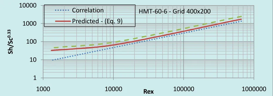
Sherwood Number vs. Local Reynolds Number
Sherwood number is defined on the basis of computed condensation mass flux as ܵℎ,௫,௦௦= ሶ
,, ഐವ
ೣ (௪್ି௪ೢ)
(9)
The local Reynolds number and Schmidt numbers are defined as [4] ܴ݁௫=௪ഥೌ௫
ν (10)
ܵܿ=
ν
(11)
Where Sh = Sherwood number
݉ሶ,, = mass transfer rate (kg/m2s)
ρ = density (kg/m3)
0 0.02 0.04 0.06 0.08 0.1 0.12
0 0.2 0.4 0.6 0.8 1 1.2 1.4 1.6 1.8 2
C o n d e n sa ti o n M a ss F lu x (k g /m 2s) Height (m)
Condensation Flux
HMT-30-3HMT-60-3 HMT-30-6 Velocity Wall Temperature 0 1 2 3 4 5 6 7
0 0.05 0.1 0.15 0.2 0.25 0.3
V e lo ci ty ( m /s )
Outlet Face (m)
HMT-30-3 HMT-60-3 HMT-30-6 HMT-60-6
D= diffusion coefficient (m2/s) x = axial co-ordinate (m) w = mass fraction of steam Rex = Reynolds number
ν = kinematic viscosity (m2/s)
ݓഥ = average channel velocity (m/s) Sc = Schmidt number
Figures 9 to 12 show the predictions for the four cases viz. HMT-30-3, HMT-60-3, HMT-30-6 and HMT-60-6 obtained from the present analysis. The analysis predictions using two definitions of sherwood number are compared with the correlation based on analogy between heat and mass transfer. The predictions for all cases are in good agreement with the correlation. The legend ‘predicted-(Eq. 9)’ indicates that the Sherwood number is calcualted from the Eq. 9. The legend ‘predicted – (Eq. 12)’ indicates that the Sherwood number is calcualted from the Eq. 12. The definition of sherwood number used by Ambrosini et. al (2008) is as follows.
ܵℎ,௫,௦௦ = ሶ,, ഐವ
ೣ ൬భషೢೡ,್భషೢೡ,൰
(12)
Fig. 9: Sh/Sc0.33vs. local Reynolds number (HMT-30-3)
Fig. 10: Sh/Sc0.33vs. local Reynolds number (HMT-60-3)
1
10
100
1000
10000
100
1000
10000
100000
1000000
S
h
/S
c
0
.3
3
Rex
Correlation
Predicted - (Eq. 9)
Predicted - (Eq.12)
HMT-30-3 - Grid 400x200
1
10
100
1000
10000
100
1000
10000
100000
1000000
S
h
/S
c
0
.3
3
Rex
Fig. 11: Sh/Sc0.33vs. local Reynolds number (HMT-30-6)
Fig. 12: Sh/Sc0.33vs. local Reynolds number (HMT-60-6)
CONCLUSION
A condensation model without explicitly considering the film was developed and implemented in the FLUENT CFD code through user defined functions. The model was benchmarked against the idealized version of the CONAN test facility. Sensitivity study was carried out to arrive at the best suited grid. The predictions were compared with the correlation based on heat and mass transfer analogy and are found to be in good agreement.
REFERENCES
[1] Houkema, M., Siccama, N.M., Lycklama Nijeholt., J.A., Comer, E. M. T., “Validation of the CFX4 CFD code for containment thermal hydraulics”, Nuclear Engineering and Design, 238, pp.590-599, 2008.
[2] Ambrosini, W., et. al., “Comparison and Analysis of the Condensation Benchmark Results”, The 3rd ERMSAR-2008, 23-25, September 2008.
[3] Vargaftik, N.B., Vinogradov, Y.K., Yargin, V.S., 1981, Handbook of Physical Properties of Liquids and Gases, Second edition, 1981, Hemisphere Publishing Corporation, New York.
[4] Ambrosini, W., Forgione, N., Manfredini, A., Oriolo, F., “On various forms of the heat and mass transfer analogy: Discussion and application to condensation experiments”, Nuclear Engineering and Design, 236, pp.1013-1027, 2006.
1
10
100
1000
10000
1000
10000
100000
1000000
S
h
/S
c
0
.3
3
Rex
Correlation
Predicted - (Eq. 9)
HMT-30-6 - Grid 400x200
1
10
100
1000
10000
1000
10000
100000
1000000
S
h
/S
c
0
.3
3