Performance Comparison of Transmission Waveforms for Active Sonar Detection

Performance Comparison of Transmission

Waveforms for Active Sonar Detection

C. K. Sunith

Assistant Professor, Dept. of Electronics, Model Engineering College, Thrikkakara, Kochi, Kerala, India

ABSTRACT: An active sonar system gathers information about a target by processing the received echo from the target. In active sonar systems, estimates of space-time co-ordinates of the target including range and velocity information are obtained by observing the effect the target has on the parameters of the transmitted signals. The received signal is processed with the help of a matched filter, their output being the prime source of target information. To develop an active sonar system, information is required on the desired properties of the waveforms transmitted by the system. The choice of waveform will determine the ability of the system to extract information concerning range and velocity resolution. The central theme of the work carried out here was to simulate using Matlab and explore the possibilities of the use of a better waveform based on resolution, environmental and mutual interference criteria. As much as six waveforms have been compared for their performance characteristics in an active sonar simulation setup.

KEYWORDS: Active Sonar, Matched Filter, Range Resolution, Doppler Resolution, Reverberation Level, Mutual Interference, Doppler Sensitivity, Costas Codes, Cox Comb, Quadratic Congruence Codes.

I. INTRODUCTION

Sonar is the abbreviation for “Sound, Navigation and Ranging.” It was developed as a means of tracking enemy submarines during the Second World War. An active sonar system essentially consists of a transmitter, transducer, receiver and display. An electrical impulse sent from the transmitter is converted into a sound wave by the array of producers and transmitted into the water. This wave strikes the target and rebounds. Echo from the target is received back by an array of hydrophones, which converts it back into an electric signal. The signal so received is amplified, processed by the receiver and sent to the display. Since the average speed of sound in water is approximately 1500 meters per second, the time lapse between the transmitted signal and the received echo can be measured and the distance to the object determined. This process repeats itself many times per second. The performance of an active sonar system has strong dependence on the type of waveform transmitted and is thus a subject matter of continued investigation. Range Resolution and Doppler Resolution are complementary. Range resolution is proportional to bandwidth. Active sonar performance depends also on reverberation rejection. Hence, the ability of a waveform to reject reverberation and noise is of utmost importance. Multiple active sonar systems operating within the same premises will give rise to mutual interference. The transmitted waveform shall not be subjected to a high degree of mutual interference; hence the choice of a waveform that is less affected by mutual interference is essential. Estimation of degree of mutual interference between waveforms will hence assume due importance.

II. RELATED WORK

Radar Waveforms and their properties have been discussed at length by Levanon et.al.[1] in their textbook. Winder et.al.[2] in their work have described an Active Sonar System and the use of waveforms in Active Sonar Systems. An analysis of CW and LFM for use in Active Sonar Systems has been conducted by Glisson et.al.[3] in their work. Costas et.al.[4] in his work has described the properties of Costas Coded Waveforms. Sum et.al.[5] in their paper has mentioned about the properties of Cox Comb Waveforms. An algorithm for normalisation of Sonar data described by Baldacci et.al.[6] was used in this work.

that were applied to this receiving chain. Section V lists down the arithmetic expressions used to arrive at conclusions, while section VI explores the simulation results. The paper concludes with the expression of hope for the emergence of new and better waveforms that essentially suits all the requirements for active sonar applications.

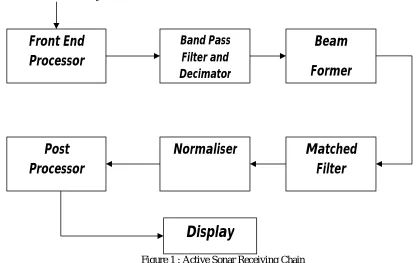
III. ACTIVE SONAR RECEIVING CHAIN

The front end processor conditions the array signal and converts it to digital signals for processing. The receiver (Figure 1) has to process the signal at lesser data rates. The signal is bandpass filtered to improve SNR. Decimation process helps to sample the signal at a lesser data rate convenient to the receiver. The beamformer comprises of a series of receiving elements or hydrophones. Receiving arrays are linear assemblies of hydrophones designed to enhance directivity and improve signal to noise ratio. Array Weights and shading coefficients are multiplied with the received signal to account for the attenuation suffered, to improve the directivity and to account for phase/time difference between different receiving elements depending on maximum response axis. Chebyshev polynomial coefficients were used as shading coefficients to suppress side lobe levels to as low as 23 dB below main lobe level.

From Transducer Array

Figure 1 : Active Sonar Receiving Chain

A Normalisation algorithm[6] was used to estimate and remove noise, and to make the noise background time invariant.

IV. PULSE TYPES

The idea was to generate pulse of duration 0.5 seconds on and 0.5 seconds off (a total of 1 second duration) using Matlab, combine noise (white, Gaussian), reverberation as well as interference with the transmitted signal, process the combined signal using the receiver chain previously mentioned, observe their matched filter[1] responses and estimate their Reverberation Levels (RL) as well as mutual interference characteristics. The waveforms considered were Pulsed Continuous Wave (CW), Linear Frequency Modulated[3] (LFM), Sinusoidal Frequency Modulated[7] (SFM), frequency hopped pseudo random noise (PRN) sequences based on Costas codes[1,4] and

Front End

Processor

Band Pass

Filter and

Decimator

Beam

Former

Matched

Filter

Normaliser

Post

Processor

Geometric Comb[5] (Cox Comb) waveforms and waveforms based on Quadratic Congruence Codes (QCC). The centre frequency of CW and modulated waveforms was set to 10 KHz. The receiver bandwidth was set to 400 Hz.

V. WAVEFORM ARITHMETIC

The correlation of Doppler shifted stored reference with the received signal forms the matched filter response of a waveform. The matched filter responses and the observed parameters form the basis for the selection of a waveform suitable for active sonar detection. Range and Doppler resolutions are computed from the 3dB widths of the matched filter responses. Range resolution is given by the expression:

∆R = c∆τ/2 (1)

where c is the average sonic velocity in sea water and ∆τ is the 3dB width of the matched filter response. Doppler

resolution may be expressed as:

∆V = c/(2f0∆τ) (2)

where f0 is the centre frequency of the waveform.

The detection capability of various ping types versus active signal spectrum reverberation may be modelled using Q-function, which is simply the integration of the ambiguity function along the range axis; i.e., the ability of the signal to discriminate against targets with different Doppler. Q-function is related to reverberation level (RL) by the expression:

RL= F(u0)Q(δf0) (3)

F is a function of range, δ is the Doppler parameter, f0 the center frequency, and Q is the Q-function at range u0 and

Doppler shift δf0. Hence a plot of reverberation levels become necessary to assess the performance of a waveform in a

reverberation limited environment. A normalised logarithmic scale (base10) in decibels has been used for generating comparative merits of reverberation levels. Reverberation levels have been normalised to the total signal energy. The ratio of cross correlation of the stored replica to the interfering signal (or the matched filter response to the interfering signal) to the autocorrelation of the transmitted signal forms the criteria for comparison of waveforms in terms of mutual interference rejection.

A waveform is said to be Doppler sensitive if its matched filter response peaks only at the expected values of the delay and Doppler parameter combination[3]. Doppler parameter (delta, δ) is given by the expression

C

V

2





where V is the target velocity, C the sonic speed in water whose average value is equal to 1500 m/s. The expected

value of δ was assumed to be 0.02 in this work. A waveform is said to be Doppler sensitive[3,8] if its matched filter response peaks only at the expected value of δ and offers very low magnitudes at other values of δ.

VI. RESULTS

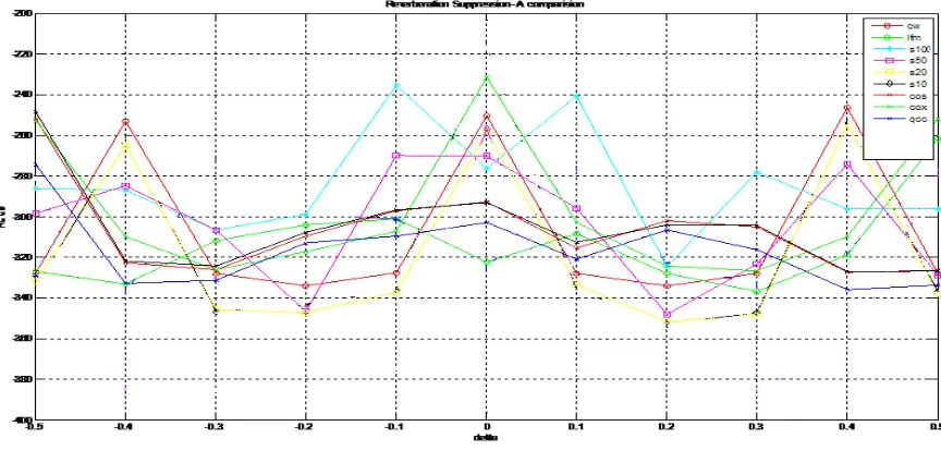
reverberation level at low values of Doppler (Figure 2) is suitable for use at low Doppler values in a reverberation limited background. The choice of correct modulation frequency is very critical for SFM[7] when compared for their reverberation performances. SFM has a series of peaks within bounds that move apart as modulation frequency is reduced. Costas coded waveforms do have optimum reverberation levels at all ranges. CW waveform has good reverberation properties at higher values of Doppler. Figure 3 shows a comparative plot of Doppler sensitivity characteristics of the waveforms under study. With δ varied from 0 to 0.04, the peak amplitudes of matched filter

output, after normalization with rms mean value of background noise were plotted along Y axis against values of delta along X axis. Simulation results show that frequency hopped waveforms based on pseudo random noise sequences, such as Costas coded waveforms, Cox Comb and waveforms based on Quadratic Congruence Codes (QCC) do exhibit good Doppler sensitivity and tend to peak only at the expected value of Doppler parameter δ = 0.02. Frequency

modulated waveforms such as LFM tend to show low Doppler sensitivity, which puts stringent demands on the choice of a detection threshold for LFM. SFM was found to exhibit good Doppler sensitivity characteristic irrespective of the choice of modulating frequency. Pulsed CW waveform also showed good Doppler sensitivity during simulations.

It is possible to have a scenario with multiple active sonar systems in the same area. It is always desirable to have an active transmit waveform that is not subject to high degrees of interference. The lower the interference, lesser the possibility of either jamming or target detection error. The matched filter response to a similar or a different signal of another frequency gives information about the mutual interference of different transmission waveforms. The lower the value of cross ambiguity function, lesser will be the interference and better will be the mutual interference rejection capability. Table 2 shows the mutual interference rejection capability of a reference wave of 10 KHz with an interfering wave of 15 KHz of similar and dissimilar wave type obtained by the cross correlation of the reference wave with the interfering wave and expressed in decibels. The table shows the superiority of pulsed CW waveform over other waveform types in terms of mutual interference rejection characteristics. Costas Coded and Cox Comb waveforms are also not very far behind when compared for their mutual interference rejection characteristics.

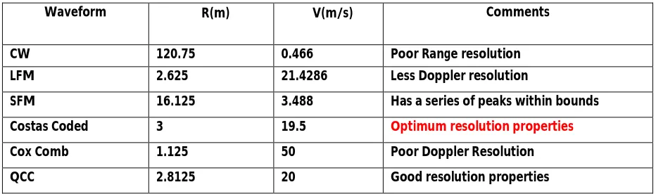
Waveform R(m) V(m/s) Comments

CW 120.75 0.466 Poor Range resolution

LFM 2.625 21.4286 Less Doppler resolution

SFM 16.125 3.488 Has a series of peaks within bounds

Costas Coded 3 19.5 Optimum resolution properties

Cox Comb 1.125 50 Poor Doppler Resolution

QCC 2.8125 20 Good resolution properties

R

e

fe

re

n

ce

W

av

e

1

0

KH

z

Cross Correlation (dB)

Interfering Wave 15 KHz

CW LFM SFM Costas CoxComb QCC

CW -47.5670 -57.0357 -53.4543 -31.476 -21.5035 -25.3199

LFM -33.8442 -46.3568 -31.7436 -3.6911 -5.6451 -12.1344

SFM -34.3240 -46.1368 -51.6394 -4.8159 -2.4573 -20.1145

Costas -38.9345 -40.3038 -38.0285 -16.5907 -33.1984 -21.9129

Cox Comb -40.7635 -36.6484 -39.6296 -17.6507 -27.8917 -16.9975

QCC -29.9593 -30.7554 -29.4574 -13.7795 -32.3134 -11.7630

Table 2: Cross Correlation (dB) for Mutual Interference Rejection

Figure 2: Doppler Parameter Delta versus Reverberation Level : A Comparison (s100 – SFM Modulation Frequency 100 Hz, cos- Costas Coded)

CW

S100

S50

S20

S10

Cost

Cox

QCC

Figure 3: Doppler sensitivity of waveforms, [S<XXX>/S<XX> : SFM<Modulating Frequency, Hz>]

VII. CONCLUSIONS

The theoretical performance of several types of active sonar waveforms was investigated. Waveform design has been a potential candidate for continued research in the field of radar and sonar. Military research establishments world wide continually strive to figure out better or improved waveforms that essentially suit almost all requirements. Still, there has to be tradeoffs in the choice of a waveform, since there is no such waveform that can be considered as ‘ideal’ - a waveform that ideally suits resolution, sensitivity, signal quality, reverberation and mutual interference requirements of active sonar systems at almost all values of ranges and velocities. Implementation of a better waveform that suits all these requirements is still a subject matter of further research. Extensions of the work may include further analysis based on signal quality characteristics such as Signal to Noise Ratio and Signal to Reverberation Ratio as well as the probability of detection. Simulation results show that frequency hopped waveforms based on pseudo random noise sequences such as Costas codes tend to offer optimum performance in terms of parameters. However, implementation of an adaptive algorithm wherein the system senses the environment and transmits the desired waveform accordingly will certainly enhance the performance of an active sonar system.

REFERENCES

1. Levanon, Nadav and Mozeson N , “Radar Signals”, IEEE Press , John Wiley and Sons.

2. Winder, Alan A, “Sonar System Technology”, IEEE Transactions on Sonics and Ultrasonics, Sept 1975.

3. Glisson, Black and Sage, “On Sonar Signal Analysis”, IEEE Transactions on Aerospace and Electronic Systems, January 1970.

4. Costas,John P , “A Study of Class of Detection Waveforms having Nearly Ideal Range Doppler Ambiguity Properties”, Proceedings of IEEE, August 1984.

5. Sun, Collins & Xiao, University of Birmingham, “Target Tracking Using Wideband CoxComb Waveforms for Human Computer Interaction”. 6. Baldacci, Alberto & Haralabus, Georgios, “Adaptive Normalisation of sonar data”, NURC-PR-2006-13, August 2006.

7. Sunith, C K, Choice of Modulating Frequency of SFM in Active Sonar Applications”, IETE Journal of Education, Volume 52, No. 1, January – June 2011.

8. Ricker, Dennis W, “The Doppler Sensitivity of Large TW Phase Modulated Waveforms”, IEEE Transactions on Signal Processing Vol. 40, No. 10, October 1993.

BIOGRAPHY