Issues involved in the empirical testing of a multivariate predictive system.

University of Windsor

University of Windsor

Scholarship at UWindsor

Scholarship at UWindsor

Electronic Theses and Dissertations

Theses, Dissertations, and Major Papers

1-1-1974

Issues involved in the empirical testing of a multivariate predictive

Issues involved in the empirical testing of a multivariate predictive

system.

system.

Robert T. Forsyth

Follow this and additional works at: https://scholar.uwindsor.ca/etd

Recommended Citation

Recommended Citation

Forsyth, Robert T., "Issues involved in the empirical testing of a multivariate predictive system." (1974). Electronic Theses and Dissertations. 6715.

https://scholar.uwindsor.ca/etd/6715

This online database contains the full-text of PhD dissertations and Masters’ theses of University of Windsor students from 1954 forward. These documents are made available for personal study and research purposes only, in accordance with the Canadian Copyright Act and the Creative Commons license—CC BY-NC-ND (Attribution, Non-Commercial, No Derivative Works). Under this license, works must always be attributed to the copyright holder (original author), cannot be used for any commercial purposes, and may not be altered. Any other use would require the permission of the copyright holder. Students may inquire about withdrawing their dissertation and/or thesis from this database. For additional inquiries, please contact the repository administrator via email

This reproduction is the best copy available.

by

ROBERT T. FORSYTH B.A.,Brock University,1973

A Thesis

Submitted to the Faculty of Graduate Studies through the Department of Psychology in Partial Fulfillment

of the Requirements for the Degree of

Master of Arts at the University of Windsor

Windsor,Ontario,Canada

1974-UMI Number: EC53126

INFORMATION TO USERS

The quality of this reproduction is dependent upon the quality of the copy

submitted. Broken or indistinct print, colored or poor quality illustrations and

photographs, print bleed-through, substandard margins, and improper

alignment can adversely affect reproduction.

In the unlikely event that the author did not send a complete manuscript

and there are missing pages, these will be noted. Also, if unauthorized

copyright material had to be removed, a note will indicate the deletion.

®

UMI

UMI Microform EC53126

Copyright 2009 by ProQuest LLC.

All rights reserved. This microform edition is protected against

unauthorized copying under Title 17, United States Code.

ProQuest LLC

789 E. Eisenhower Parkway

PO Box 1346

Ann Arbor, Ml 48106-1346

Dr.

Dr.

Dr.

Dr.

M. Morf

APPROVED BY:

/ / u ■ ^

/ f i , j i

-H. Minton / f - >

R. Daly

S. Sadava

ii

This study utilized previously collected data from two

samples of 187 and 184 college students to investigate problems

inherent in multivariate data analysis as well as patterns of cannabis

use. The multivariate issues considered were: the effects of the

distributions of the scores of the variables; the use of factor

scores as well as raw data in regression analysis to facilitate

"conceptual cross-validation"; effects of sequential orthogonalization

on regression equations; and the utility of criteria exhibited by

factor analyses and canonical correlations. It was found that in

the field of marijuana research, the usual criterion - frequency of

use, was not suitable both for measuremeant and inferential reasons.

Using canonical analysis two patterns of use were found -- moderate

and abnormal, which were related to social and personality predictors

ACKNOWLEDGEMENTS

I acknowledge the help of the members of my committee:

M. Morf, H. Minton, R. Daly, and S. Sadava.

Appreciation .is

also extended to Marybeth Heilbronn and Larry M. Starr.

Page

ACKNOWLEDGEMENTS ... iv

LIST OF TABLES ... ... vi

LIST OF FIGURES ... vii

Chapter

II METHOD ... 13

III . RESULTS ... 23

IV . DISCUSSION ... 41

V CONCLUSIONS ... 58

Appendix A Proof for Gamma Scores ... 64

Appendix B Programmes Written for this Thesis ... 65

Appendix C Correlation Matrices ... 67

REFERENCES ... 75

VITA AUCTORIS ... 78

LIST OF TABLES

Table

1 Variables Used , ... 14

2 Univariate Distributions ... .. . . . . 24

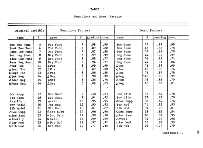
3 List of Factors for Functions and Demo. ... 28

4 Factor Loadings of Criteria ... 32

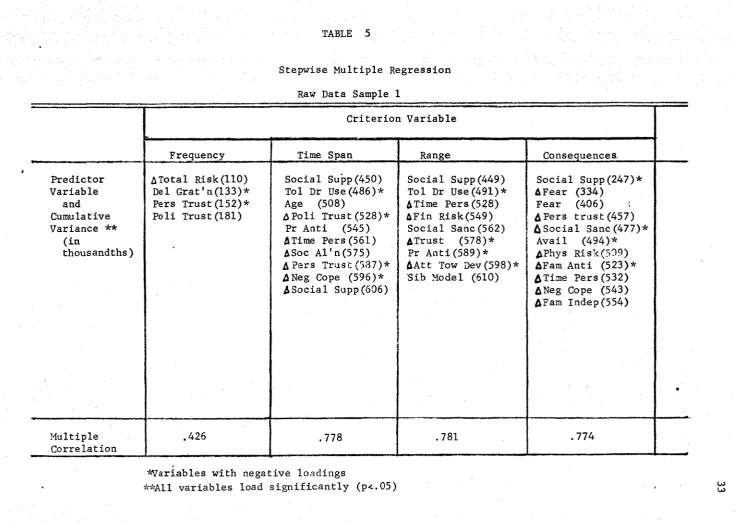
5 Stepwise Multiple Fegression,Raw Scores,Sample 1 . . . . 33

6 * Stepwise Multiple Regression,Raw Scores,Sample 2 . . . . 34

7 Stepwise Multiple Regression,Functions Factors,Sample 1 . . . 35

8 Stepwise Multiple Regression,Functions Factors,Sample 2 . . . 36

9 Stepwise Multiple Regression,Demo. Factors,Sample 1 . . . . . 37

10 Stepwise Multiple Regression,Demo. Factors,Sample 2 38 11 Summary of Multiple Correlations . ... 39

12 Canonical Correlations . . ... 40

vi

Figure Page 1 Simple, Non-Recursive, Social Learning Mo d e l ... 5 2 Scattergrams... . 25

Chapter I Introduction

One of the major aims, if not the only aim of psychology, is useful

and accurate prediction of human behaviour. The approaches used vary

with the particular behaviours studied, ranging from the study of minute

reflexes, to overall life patterns, carrying with them constructs from

conditioned stimuli to self-concept. For behaviour of medium complexity, the social learning approach, developed by Rotter and his colleagues

(eg. Rotter, 1954; Rotter, Chance & Phares, 1972) or a similar approach may be most useful, provided that constructs are made sufficiently clear.

It is the intent of this thesis to operationalize some of these constructs, to investigate methods of testing a predictive system, and to consider

specific issues that pertain to this system and generally to complex multi ­ variate data sets.

In this study the behaviour of interest is marijuana use, specifically

in college students. Studies on the drug have proliferated, perhaps in

keeping with greater public interest in its use and abuse in the last few years. Although much of the literature deals with the physiological and psycho-pharmacological properties of cannabis, the psychological viewpoint

demands an exploration of social and personality correlates and the consequent predictions of who uses the drug, and with what effects. Recent studies

by Jessor (Jessor, Jessor & Finney; 1973) and Sadava (1974b) have had some success in this task, by viewing marijuana use as a functional

behaviour, "caused" by variables both of an interpersonal (environmental)

and of an intrapersonal (personality) nature, and as an ongoing process

1 ; .

changing over time. This conception of the problem may be traced back to Rotter's social learning framework, and a short description of this

approach (based mainly on Applications of a social learning theory of

personality, chapter 1, 1972) would make the later work more meaningful.

Rotter's Social Learning Theory ■ ,f

In general, Rotter's Social Learning Theory utilizes the ideas of

expectancy and the empirical law of effect, as underlying constructs emphas­

izing the interaction of the individual and his meaningful environment. Thus, the approach is much more cognitive in nature than most other types

of learning theory. Specific efforts are directed to determmm^ the subject's

perceptions of his goals and his subjective .< expectancy that they will be

fulfilled according to his own past experiences. Needs and goals are social in nature since they are initially fulfilled by others. Behaviour

becomes available if it has led to reinforcement, either directly, or

through observation and modelling. Generalization takes place, with functionally related behavious/reinforcers leading to the same goals/

satisfactions. Cognitions are more important in this theory than others

since the generalization may be of symbols and their referents. The general formula used to predict behaviour is: BP=f(E & RV) where BP is

the probability of the behaviour, relative to other behaviours in the

specific (psychological or perceived) situations; E is the expectancy or subjective probability of a particular reinforcer occurring as a

result of a certain behaviour; and RV, the reinforcement value, is the relative preference for a given reward with expectancies for all rewards

kept constant.

3

college,in relation to peer approval, is a function of the expectancy of the occurance of peer approval, following marijuana smoking in college

and the value of peer approval. This is a specific example, and may be

expanded by including other reinforcements, both positive and negative,

other expectancies etc.

Jessor*s Approach

Jessor has taken Rotter's system, developed in a clinical setting, and applied it to studies on alcohol use (eg. Jessor, Carnan, & Grossman,

1968; Jessor & Finney, 1973). Marijuana use is thought of as "problem

behaviour... considered to be purposeful, goal oriented or functional (pi,

1973)". Variables have been classified into structures and systems by Jessor; a personality system consisting of motivational instigation, belief and personal control structures; a perceived environment system

with these and other behaviours ranging from closely related to "normal".

His methodology consists of administering questionaires at two or more

points in time, using multiple-regression techniques, and gain scores (over time), on social and personal variables to increase "accounted-for"

variance. He was able to assign users and non-users to their respective groups with 73% accuracy and to achieve multiple R's of up to .39 (Jessor,

et al, 1973).

Sadaya's Approach

Sadava's approach has focused in on marijuana use specifically. One

major problem in marijuana research is that while ultimate clinical interest may lie in determining what leads to abuse, research has been defined in

terms of use versus non-use. Even this distinction is made in different ways by various researchers. For instance the category of "light use"

ranges from one to twenty experiences, and there are at least twenty-eight

labels for use patterns (Sadava, 1974a). To cut down this confusion,

Sadava designed a short group of questions, with four stages of use (Sadava,

1972) with the additional stages of non-user and "Have stopped" added (Sadava 1974b). For the non-user and the four user stages this scale has

Guttman-scale type properties. Continuing to refine criteria, Sadava

uses the following measures; frequency of use, time span as a user, contexts of use and adverse consequences of use in a sample comprised of drug users. These measures have average intercorrelations of .23 with a maximum of .54

(Sadava, 1974b), indicating relationships amongst criteria, and the possibility

of patterns of drug use. The complex relationships between behaviour and

predictors may be obscured by a poor choice of criterion. Meaningful correlate may be hidden from our investigation if the criterion is poorly defined, or

if its scale properties are ignored.

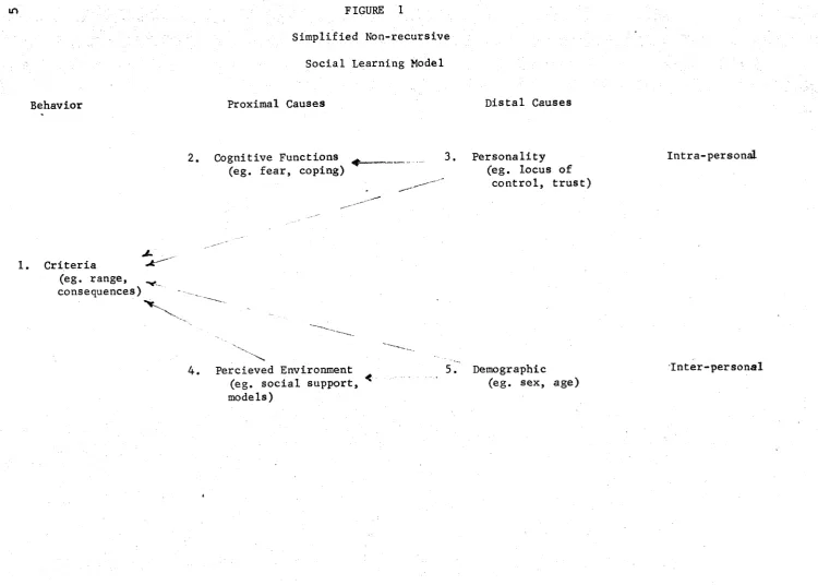
Sadava's schema of variable systems may be seen in Figure 1. The major difference between the systems of Sadava and Jessor is that in the former

cognitive functions are conceptualized as a set of predictors of drug use (by Sadava), and as being predicted by other systems of variables. Using

his system Sadava (1974b) has found multiple R's of up to .62 for variables predicting criteria measured at the same time, and multiple R's up to .58

for longitudinal analyses with samples of drug users. Both Jessor and

Sadava use longitudinal analyses, and often utilize both the scores on

variables at the earlier point in time, and change scores in these variables, to predict behaviour at the second point in time.

Social Learning Theory: Applied to Complex Operations

m FIGURE 1

Simplified Non-recursive

Social Learning Model

Behavior Proximal Causes

Criteria (eg. range, consequences)

2. Cognitive Functions ^ _ (eg. fear, coping)

4. Percieved Environment (eg. social support, models)

Distal Causes

Personality (eg. locus of

control, trust)

Demographic (eg. sex, age)

system that would allow easy manipulation of the large number of variables

and extensive data. Thus the first stage of this thesis is the expression of Sadava's and Jessor's systems in a notation that allows manipulations pf

s

variables in order to deduce and to subject to verification, hypotheses

about relationships between predictors and criteria. This is a necessary step since some of the terms used (eg. 'related structures', 'covary with

other kinds of problem behaviours') and also relationships between

variables (eg. BP=F(E & RV)) are hard to operationalize. Furthermore,

although the underlying principles assume an integrated predictive system, the tendency is to examine concepts and variables in isolation, and with

less than complete thoroughness. Notation

Let B „ be a criterion observation ["section 1 of Figure ll for

qtn L ,

individual n (n=l,...,N) at time t (t-1,...,T) on criterion q (q=l,...,Q) which after appropriate transformations(s) is in Z-score form (Exp (Bq t n )=0,

Var(Bq t n )=l). Similarly, let C ltn(l=l,...,L) be a normalized variable for cognitive functions [section 2 of Figure ; P ^ (m=l,.... ,M) be a normalized variable for personality characteristics (section 3 Figure lj ;

E (k=l,...,K) be a normalized variable for perceived environmental data ktn

^section 4 Figure l j ; and Dstn(s=l,...,S) be a normalized variable for

demographic data (section 5 Figure l~J.

Let A( B q tn) be a normalized variable corresponding to the unpredicted

part (i.e., change over time-delta) of Bqfcn from Bq ^n - Similarly, A ^ l t n ^ ’

7

Let Fr n (B) be the factor score for the r'th factor (r=l,... ,R). for individual n, taken from the B ^ (D).

’ q t n N '

covariance-free part (gamma) of Pm |-n remaining after the variance due to

the E and C variable systems is partialled out, and so on for combinations

of P, E, C and D.

bet R g q g Q p be the multiple correlation between the qth variable of

B and the variables of E, C and P.

Thus using the above notation for measurement tines 1 and 2, it is

hypothesized that an equation of the following general form leads to better

estimations of criteria at time 2 and higher multiple R's than obtained previously:

The score for the n'th person, on the q'th criterion, at time 2, may be estimated from a linear composite comprised of the sum of the variables in each system weighted such that the predictors are orthogonal. Thus in this case, the estimated criterion score is the sum of the factor scores for demographic data weighted by first order correlation coefficients with

Let f ^ C E H C ) denote a normalized variable consisting of that

A

the criterion, plus the sum of the personality factor scores, free of covariance with demographic data, and weighted by the correlations with the criterion, plus the percieved environment factor scores similarly

partialled (of both demographic and personality scores) and weighted, plus cognitive function factor scores treated in the same manner.

Problems with this Predictive System

In the present study several important limitations exist and should be

noted beforehand. Firstly, the model calls for all variables to be normally distributed, zero mean, and unit variance. This condition may not be met

because of several considerations in the scales involved; measures may be nominal or at best polychotomous with very discrete values found for

what may or may not be underlying continuous variables; some variables may be extremely skewed, and even with transformations may not really r e ­

semble a normal distribution.

A second deviation from the model relates to the fact that the various systems of variables should include all non redundant measures in the

domain of interest. This condition is not fulfilled as: (a) those measures may not at this point in time exist and (b) only a limited subset (hopefully

representative) can be administered in the time permitted.

Another problem exists in that the model is linear in nature whereas either the real or theoretical variables may combine multiplicatively in the form of moderators to other variables, or in other non-linear combinations (eg. curvilinear). This must be kept as a consideration in the research, but as the non-linear models tend to be limited operationally more or less to small numbers of variables, the present work will (hopefully)

9

Other problems exist in the nature of the instruments used and

the type of behaviour studied. In the latter case, marijuana use is,

of course, illegal and therefore responses to questions about its use can

be seen as incriminating. King (1972) reports that anonymous and

identifiable > questionnaires on this subject do not significantly differ

on reported data, however this does not mean there will be no difference between actual behaviour and reported behaviour due to some fear of exposure.

With respect to questionnaire studies in general, we must consider the possibilities of response styles and sets (eg. Jackson, 1967), and also

false content through misconceptions on the part of the subject. The latter is more easily dealt with, in that according to the assumptions of the Rotter, Jessor and Sadava models behaviour is determined by sub­

jective expectancies, values, etc. not merely objective facts, and distortion

of this kind do not render the information invalid.

To compare the possible distortion of responses on the questionnaire, it is best to consider that the data have two different logical sequences. The first sequence is that of cognitive functions followed by perceived environment, personality and demographic data, ordered in terms of

decreasing proximity to the behaviour concerned. The subjects' own

perceptions will have the most weight and be least subject to cumulative

response biases.

The second sequence will be that of demographic data, personality, perceived environment, and cognitive function, in decreasing order of objective verifiability, as opposed to proximal subjectivity.

Specific Areas of Investigation

There are four specific issues that must be examined in dealing with

the model. These are: distributional properties of predictor and

criterion variables; the use of raw data vs factor scores; the use of

two sequences of orthoganalization, ie. starting with cognitive functions,

and starting with demographic variables; and the patterns of behaviour criteria.

Distributions of the Variables

It is extremely important that we examine the distributions of scores

on the variables we use before interpreting results from statistical

analyses, since we may be misled by our results if assumptions necessary

to the analysis are not met, or if more useful approaches to data analysis

are ignored due to a lack of information. This warning takes on more importance when the variables haven't been used extensively in other

research, and/or several "non-robust" (requiring stringent assumptions for use and interpretation) statistics such as stepwise regression or canonical

correlation are to be used. For instance, we might have a distribution

with a few extreme values at each end, being correlated with another variable that also has extreme values. If the extreme values "match", there will

be a very high correlation that is not reflected at all by the other

variable pairs. Another possibility is that the two variables have a parabolic relationship, or that one variable is related to the logarithm

of the other. In both cases, the correlations between the variables would be very low, and the true relationships found only by a theoretical or, more likely, an empirical investigation of the univariate and bivariate

frequency distributions of the variables (see Carroll, 1967). As the

first part of the exploration of this model, these distributions will

1 1

Raw Data vs Factor Scores

Since the scales for this investigation were chosen on the basis of availability, or constructed to measure a specific area, there may be

both a large overlap in the domain of measurement, and a great deal of variance "superfluous" to the model. If the variables are of this

nature, the use of a multiple regression technique may lead to different weights for the variable in each sample, even though the particular Under­

lying factors don't change from sample to sample. Cooley and Lohnes (1971) point out that "chance" is an important consideration in multivariate

analysis, and since we may have several variables contributing almost the

same variance, chance could determine which variable is chosen (the

covariance with similar variables being partialled out and consequently not appearing as significant). This process may have more importance than

seems readily apparent since we will be influenced in our model building and generalization by the labels or names attached to the "significant"

variables, and may draw the wrong inference about the meaning of a variable's loading on the regression equation.

One solution to this problem is to assure ourselves, prior to the dependence analysis (eg. multiple regression), that we have predictors, whose domains, empirically, do not overlap greatly. This may be achieved

by orthogonalization of our predictors. We may also collapse the number of variables into a smaller number of factors. Using this method, we may substantiate the findings of analyses of raw data, and more easily

infer from the measured variable the underlying trait or cause. Sequence of Data Entry

When orthogonalizing the data sequentially, the first variables may

retain greater meaningful variance than later variables because of the method itself. The last variables will, most likely, have little or no correlation with the criterion, whereas the corresponding original variable may, in reality, be highly related to the criteria. Ideally every variable

should have equal chance to covary with criteria, but this leads to an enormous number of analyses to include each sequential combination. Given

these circumstances, together with the theoretical reasons discussed

previously for the different types of response sets and kinds of verifiability two sequences of orthogonal predictors will be used: Functions- in which

the function variables are entered first (the sequence of proximity); and Demo.- in which the demographic variables are entered first (the objective verifiability order). These sets will be examined to determine what

differences exist due to ordering effects. Criteria Patterns

Considering Sadava's findings (1974b) concerning the relationships between criteria, and the different predictors useful in each case, it is

important to look at the criteria carefully, to examine specifically their

inter-relationships (eg. by factor analysis), and to find out whether different sets of predictors predict different patterns of criteria

(using canonical correlation). Using this information we can evaluate the criteria as to their reliability and usefulness. In addition, a methodology becomes available to ascertain predictive systems for genuine, multidimensioiu

Chapter II Method

Subjects

The •’uestionnairee were filled out by first and second year students enrolled full-time at Brock University, St, Catharines, Ont. in the

1972-73 academic year. Pour hundred and eighty Ss_ completed question-aires in Nov. 1972; and of these 371 filled out the questionnaire in Mar. 1973. The ages of the Ss_ ranged from 16 to 74 but most were under

26. Fifty-five per cent of those responding twice were female.

The group (371) was split into two samples randomly, Sample 1 was 187 Ss_ and Sample 2 was 184. Scores were standardized within samples, but all other estimated parameters-(e.g. correlations, factor loadings, etc.) were obtained from Sample 1 and applied to Sample 2 .

Questionnaire

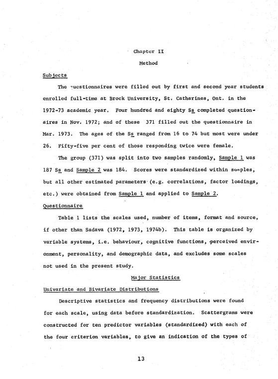
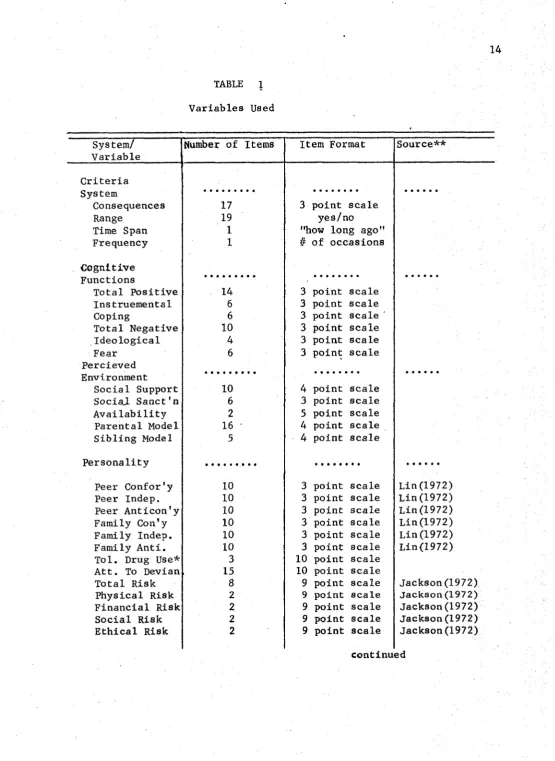
Table 1 lists the scales used, number of items, format and source, if other than Sadava (1972, 1973, 1974b). This table is organized by

variable systems, i.e. behaviour, cognitive functions, -perceived envir­ onment, personality, and demographic data, and excludes some scales

not used in the present study.

Major Statistics Univariate and Bivariate Distributions

Descriptive statistics and frequency distributions were found for each scale, using data before standardization. Scattergrams were

constructed for ten predictor variables (standardized) with each of the four criterion variables, to give an indication of the types of

13

Variables Used

System/ Variable

Number of Items Item Format Source**

Criteria System

Consequences 17 3 point scale

Range 19 yes/no

Time Span 1 "how long ago"

Frequency 1 # of occasions

Cognitive Functions

Total Positive 14 3 point scale Instruemental 6 3 point scale

Coping 6 3 point scale

Total Negative 10 3 point scale Ideological 4 3 point scale

Fear 6 3 point scale

Percieved Environment

Social Support 10 4 point scale SociaJ. Sanct'n 6 3 point scale Availability 2 5 point scale Parental Model 16 ■ 4 point scale Sibling Model 5 4 point scale Personality

Peer Confor'y 10 3 point scale L i n (1972) Peer Indep. 10 3 point scale Lin (1972) Peer Anticon’y 10 3 point scale L i n (1972) Family C o n ’y 10 3 point scale Lin(1972) Family Indep. 10 3 point scale L i n (1972) Family Anti. 10 3 point scale L i n (1972) Tol. Drug Use* 3 10 point scale

Att. To Devian 15 10 point scale

Total Risk 8 9 point scale Jackson(1972) Physical Risk 2 9 point scale Jackson(1972) Financial Risk 2 9 point scale Jackson(1972) Social Risk 2 9 point scale Jackson(1972) Ethical Risk 2 9 point scale Jackson(1972)

15

Table 2 continued System/

Variable

Number of Items Item Format Source**

IE Locus of Con 23 Forced Choice Rotter (1966) IE personal 9 Forced Choice M i r e l s (196 ) IE political 4 Forced Choice Mirels(196 )

Trust 25 5 point scale Rotter(1966)

Personal Trust 6 5 point scale Political Trust 8 5 point scale

Interper'l Al.'n 10 5 point scale Keniston(unp) Social Alien'n 5 5 point scale Keniston(unp)

Moral Judge.* 35 mixed

Religiousity* 3 mixed

Delay Grat'n 4 5 point scale Stuffiphauser(1972) Time Pers've 5 number of months Shybut(1968)

Demographic

Sex * 1

Age * 1

Social Econ.*

Yr in College* 1

Poli. Orien'n* 1

Residence* 1

Reference Gr.* 1

Height *

Weight *

Self Des. Obs.* 1

Exp. GPA * 1

GPA Difference*

*Not repeated Spring, 1973 ** If other than Sadava

bivariate distributions present in the data.

Orthogonalization of Data

Delta and gamma scores. In order to arrive at a set of mutually independent predictors several types of transformation are needed.

First, we must get an estimate of change-over-time scores. Given two

sets of scores on the same variable, from the same subjects, we can

}

partial out of the later score, the variance accounted for by the score taken at a point earlier in time (e.g. Jessor et al, 1973). Thus, starting with two related scores, we obtain a base score, and an independent estimate of change, a delta (A) score. Delta is estimat­

ed by Ferguson's formula t. = (Z^ - r i2Z2)/V^-~r i2 -(1971, p. 387) where Z^ is the score at the first point in time, Z£ is the same subjects'

score at second point in time, and ri2 is the correlation between Z^

and Z2 over all subjects. .

A generalization of the above formula estimates a score that is independent of more than one variable (this may be done across time, as for , or with other scores from a larger test battery). If we wish an estimate of this covariance-free score, a gamma (f*) score, we

may use the following formula;

r

*

1

.

.

.

<v irlmz„)/Vi-ZrL

<rrx*%

[see appendix A for proof3, where Z is our variable of interest, 1

Z_,...,Zn are the covariates, r is the correlation between the Z,

2’ n lm 1

scores for Zm (m=2 n) over all subjects. These scores will have E(P)-0,VAR(p)-l and will tend to a normal distribution.

1 7

factor scores. Since we are interested in linear composites with the

characteristics of mutual independence, interpretability and complete­ ness, the proper procedures for this factor analysis are: the use of

unities in the main diagonal; an adaptation of the scree test (see Cattell, 1952, for a discussion of this criterion) to determine the number of factors retained; and a varimax rotation of those factors.

We must use unities in the diagonal instead of estimates of

commun-ality since our data are not being used to infer underlying structure,

but rather, are being described by the factor scores. The question of

establishing the number of variables to be rotated is more complex. It may be resolved by considering the nature of the factor structure

and the communality of a variable. We may tegard communality as the square of a variable's multiple correlation with all the extracted factors. Thus, if each variable has a high communality after a

certain number of factors has been extracted, we may assume that each

of the common and unique factors has been obtained. For example, if

after five factors are extracted, the communality of a variable is .78, there remains to be accounted for, only 22% of the original

variable's variance in all the remaining factors.

We can always (with unities in the diagonal) account for all of the variance by taking as many factors as variables, but we most like­ ly will have "error" factors, due to faulty measurement, discrete scale values etcetera. A procedure that tends to eliminate these factors is Cattell's scree test (Cattell, 1952). A sharp drop-in eigenvalues after relatively high eigenvalues means the following eigenvalues may be neglected. The original argument by Cattell

recommended both a scree test, and a minium eigenvalue over 1.0,

however, since we are using principal components, the later requirement

may be dropped, and the requirement of high communalities added.

The varimax method of rotation is used so that each factor can

'be most easily identified as related to a few (and if possible only

one) variables. Varimax simplifies factors, as opposed to variables (Mulaik, p.259, 1972), and this means that the "output" of our trans­

formation will tend to be more easily interpretable than if we used

either a variable-simplifying or both factor and variable simplifying

rotation.

Stepwise Multiple Regression ,

This technique (SMR) is really a combifiation of regression and factor analysis (Mulaik, p.412, 1972). The first step is to correlate

the criterion with the criterion as the variable in the regression equation. The factor collinear with this variable is extracted from

the predictor matrix, and a residual correlation matrix is obtained. Then the variables (or factors since this factor analysis method-that

of Cholasky [^Mulaik p.412[] maintains a correspondence between factors

and variables),remaining are correlated with the predictor, the

corresponding factor extracted, leaving a residual matrix, and so on.

At each step a variable is added to (in occasional circumstances removed from) the regression equation, and the multiple correlation

is increased.

This process of adding (and/or removing) variables can continue

1 9

regression, the unique factors that do not correlate with the criterion, may be, for practical purposes?considered error. Either error may increase

the multiple correlation, but to such a small extent that, given the probability of measurement error, the predictive utility of the equation is diminished. Cooley and Lohnes (p.56-57, 1971) point out that SMR can capitalize on chance to a large extent, and care must be taken to replicate this procedure on another sample(s). The replicated R may shrink appreciably if too many variables are allowed in the original

equation. For our purposes, we may use an F ratio (or an equivalent

£ test) to determine whether a variable should be added to the equation. This F ratio is computed as the square of the ratio of regression

coefficient and its standard error (SPSS, 1970). Orthogonal Predictor Variables

If the correlation matrix of predictor variables is an identity matrix (i.e. the variables are correlated), the regression equation weights may be obtained directly from simple correlations with the

criterion (Mulaik, p.404, 1972). Furthermore, the square of the multiple correlation is the sum of the squares of the simple correla­

tion with the criterion. If we have orthogonal predictor variables, the order of entry of these variables into a stepwise MR is the same

as the rank order of the absolute values of the correlation coeffic­ ients, and the SMR is not necessary. In practice, a SMR can be useful in these circumstances since the correlation with real data probably will not be an exact identity matrix. Even if our regression weights

are from a non-orthogonal group of predictors, Cooley and Lohnes (p.56, 1971) point out that sample predictor-criterion correlation

coefficients of the first order may yield better predictive utility

than regression weights from more "sophisticated" processes. Canonical Correlation

Stepwise Multiple Regression may be considered a special case of canonical correlation. The problem of canonical correlation is to find

relational^ ps between a set of predictor variables and a set of criterion variables (in SMR we have a set of one criterion variable). In general, we ask if there is a combination of predictors X (a pattern) that has a high correlation with a combination or pattern of criterion Y variables. To do this we find a set of weights for the predictors such that the composite variable (W^) is maximally correlated to a composite variable Yj made up of a weighted combination of the’Y variables. A factor corresponding to is extracted from X which leaves the residuals Xr unrelated to W-^, in the same manner as the residual matrix is found in SMR. The composite V£ is treated in the same way to produce a residual

matrix Y r . This process is repeated producing (usually) m set of weights, where m is the number of variables in the smaller of the predictor and

criteria groups (see Van de Geer, 1971). We must then evaluate the sets of weights called canonical variates to find which are significant. The canonical correlation coefficient Rc can easily be misinterpreted. It is not the correlation or overlap between X and Y but between the linear composites W and V. To evaluate the "overlap" or shared variance of the two sets, we may use a statistic R , a redundancy coefficient

d

discussed by Stewart and Love (1968). For each canonical correlation there are two redundancy coefficients, one for the X variables given

2 1

variables given the composite W from the X variables ( i . e . R d y ) . R d x is calculated as the proportion of variance extracted by the factor (W )

n times the proportion of shared variance (Rc n ) between the factor and

corresponding canonical factor of the other battery (Cooley and Lohnes, p. 170, 1972). Thus we square the weights of the X variables, divide by the number of X variables, and multiply by the canonical correlation

The canonical correlation analysis can be useful in exploring

criterion patterns however it should be used in conjunction with other

measures such as the multiple correlation of each criterion (Cooley and

Lohnes, p.176, 1972), chiefly because of the complexity of the procedure, and the possible misinterpretation of results.

Summary of Programmes an’d Formulae

1. Univariate Distributions - SPSS (1970), subroutine CODEBOOK

2. Bivariate Distributions - BASIS (1971), subroutine Plot.

2

3. Delta Score - Z\z2 ~ ^Z1 " r 12z2 ^ x yi • A Fortran programme was written and an example given in Appendix B.

2

4. Gamma Scores: * (Z1 - (r lmzm )) / r lm * This was done by a Fortran programme in Appendix B.

5. Principal Components Analysis: Both SPSS (1970), subroutine FACTOR,

and SSP factor analysis ( 1970; p.429) were used, with several sets of data run on both to ensure accuracy (identical results to fifth signific­

ant digit).

7. Correlation Coefficients. SPSS (1970), subroutine PEARSON CORR was

used and compared to SSP subroutine CORRE.

8. Stepwise Mutiple Regression: SPSS (1970), subroutine REGRESSION, and

SSP programme for stepwise multiple regression (p. 419) were used and

compared.

9. Canonical Correlation: SPSS (1970), subroutine CAN CORR was used,

Chapter III Results

Univariate Distributions

The raw data may be grouped in sets of variables with common forms

of frequency distribution. These distributions seem to approximate: the normal, truncated normal, superimposed two population normal, the Poisson, the rectangular and the dichotomous or binomial distributions.

Table 2 gives examples of variables from each group, descriptive

statistics and type of distribution.

Bivariate Distributions and Correlations

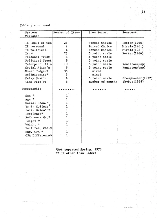
Selected pairs of standardized variables were plotted to check for usual bivariate distributions. None of the distributions seemed

curvilinear (e.g. U shaped). The scattergrams including Range seemed to indicate that extreme values (for Range) were depressing the

correlations, and suggested that correlation with Log (Range) might be considerably higher. Scattergrams are included as Figure 2.

Correlations matrices between the criteria and each of the predictor variables may be found in Appendix C. There is a matrix for each of the Raw, Functions and Demo, modes of analysis for Sample 1 and for Sample 2 .

Transforms

The resulting variables, processed in either direction, i.e., part­ ial ling out covariance of functions from social, of functions and social from personality etc; and partialling out covariance of demographic from

personality variables etc., were relatively easily identified, having

23

TABLE

Univariate Distributions

t

Central Moments * Type of

Variable**

Mean Variance Skewness Kurtosis Range Quartile ^Distribution

Frequency 17.976 6095.527 10.940 133.106 999 0/0/10 Poisson/ Dichotomous Time Span 19.505 648.855 1.365 1.860 144 0/4/36 Poisson Range 3.585 13.238 2.725 12.793 33 1/2/5 Poisson

Consequen. 31.118 116.599 0.400 -1.095 34 22/30/41 Rectangular Social Supp 19.865 36.436 0.406 -0.572 28 15/20/24 Bimodal Nor.

Avail. 8.435 2.436 -1.382 2.536 8 8/9/10 Trunc. N o r .

Sib. Model 7.557 5.433 1.675 4.733 15 6/7/9 Trunc. Nor. Total Pos. 22.862 27.451 0.491 0.156 28 19/22/26 Trunc. N o r .

Ideo. Neg. 6.470 3.432 0.799 0.159 8 5/6/8 Trunc. Nor. Fam. Conf. 22.849 6.501 • 0.053 0.079 15 21/23/25 Normal Att.To Dev. 36.891 81.661 0.069 0.472 58 31/37/43 Normal

Total Risk 38.192 89.906 0.052 0.010 54 32/38/44 Normal

I.E. 10.593 24.697 -0.014 -0.585 22 7/11/14 Normal Exp. GPA 73.843 42.218 0.511 1.014 41 70/75/80 Disc. Nor. S. D.Obes. 3.114 0.530 -0.047 0.370 4 3/3/4 Normal

Sex 1.445 0.248 0.220 -1.952 1 1/1/2 Dichotomous

* Based on 371 observations

FIGURE 2

2 5

2.00

Peer Conf.

2.00

•1.00 1.20 3.40

Time Span

2.00

Conseq­ uences

2.00

18 ₃₄

Age

continued...

2.00

Neg Funcs

0.00

-

2.00

-1.00 0.10 1.20 2.30

Range

3.40

2.00

Soc Supp

0.00

-2.00

-1.00 U 0 : * * 12.65

2 7

high loadings on principal compenwf,* analyses. Table 3 includes rotated

factor loadings, communalities, and lists new variable names for the two modes of factoring.

Factor Analysis of Behaviour

In both Samples 1 and 2, frequency is unrelated to the other

criteria, with time and range loading together. Table 4 presents

rotated loadings and eigenvalues .

Stepwise Multiple Regression Analysis

A total of 24 SMR's were calculated. Tables 5 through 10 present

the variables with significant Beta weights, the cumulative variance

in thousandths and the final multiple correlation coefficients Table 11 presents a 2 x 3 x 4 breakdown of these Multiple correlations, and

average correlations (using Fisher's Z transformation) for each

classification.

Canonical Correlations

Five canonical correlations were performed, results for canonical correlation with raw data were not obtained due to the size of the r

matrix and the programmes available. One of the canonical correlations

was meaningless due to a singular matrix resulting in a canonical

correlation greater than 1.0. Table 12 gives the significant canonical

correlations, loadings variables with loadings for each of the four meaningful analyses.

w ith pe rm is si o n of th e co py ri gh t o w ne r. Fu rthe r re production p ro h ib it e d w ith ou t p e rm is s io n .

TABLE 3

Functions and Demo. Factors

Original Variable Functions Factors Demo. Factors

Name # Name # Loading Comm. Name # Loading Comm,

Tot Pos Func 5 Pos Func 7 .99 .99 Pos Func 47 .99 .99 Inst Pos Func 6 Pos Func 7 .89 .80 Pos Func 47 .88 .78 Cope Pos Func 7 Pos Func 7 .87 .80 Pos Func 47 .88 .78 Tot neg Func 8 Neg Func 5 .99 .99 Neg Func 44 .99 .99 Ideo Neg Func 9 Neg Func 5 .89 .77 Neg Func 44 .85 .74 Fear Neg Func 10 Neg Func 5 .94 .77 Neg Func 44 .91 .84

/Tot Pos 11 4 Pos 8 .99 .99 /Pos 45 .99 .99

Alnst Pos 12 4 Pos 8 .87 .80 & Pos 45 .86 .76

A Cope Pos 13 A Pos 8 .86 .88 4 Pos 45 .87 .78

A T o t Neg 14 4 Neg 6 .98 .99 A Neg 46 .98 .99

Aldeo Neg 15 /Neg 6 .86 .76 £ N e g 46 .83 .70

AFear Neg 16 A N e g 6 .89 .83 /Neg 46 .86 .81

Soc supp 17 Soc Sane 9 .58 .83 Soc Clim 37 .84 .78

Soc Sane 18 Soc Sane 9 .94 .92 Soc Clim 37 .82 .70

Avail'y 19 Avail 15 .95 .95 ASoc Supp 38 .64 .74

Par Model 20 Par Mod 13 .95 .92 Par Mod 41 .95 .93

Sib Model 21 Sib Mod 10 .81 .87 Sib Mod 39 .78 .81

A Soc Supp 22 A S o c Supp 14 .96 .96 A S o c Supp 38 .85 .84 A Soc Sane 23 4 Soc Sane 12 .98 .98 ASoc Sane 40 .97 .95

A Avail 'y 24 A Avail 16 .99 .99 AAvail 42 .97 .96

/;Par Mod 25 A Par Mod 11 .97 .97 /Par Mod 43 .97 .99

/•Sib Mod 26 Sib Mod 10 -.77 .86 Sib Mod 39 -.74 .79

R ep ro du ced w ith pe rm is si o n of th e co py ri gh t o w ne r. Fu rthe r re production p ro h ib it e d w ith ou t p e rm is s io n .

Cont * d

Name # Name # Loading Comm. Name # Loading Comm.

Peer Conf 27 Peer Conf 27 .95 .94

Peer Indep 28 Indep 22 .87 .88

Peer Anti 29 Anticonf 21 .85 .80

Fam Conf 30 Fam Conf 30 .93 .92

Fam Indep 31 Indep 22 .87 .87 Fam Indep 29 .98 .99

Fam Anti 32 Anticonf 21 .87 .86 Anticonf 21 .97 .98

Att Tow Dev 33

To I Dr Use 34 Tol Dr Use 27 .96 .95 Tot Risk 35 Tot Risk 20 .90 .87 Phys Risk 36 Tot Risk 20 .91 .87 Fin Risk 37

Soc Risk 38 Soc Risk 20 .98 .99

Eth Risk 39

Tot I-E 40 I-E 17 .94 .95

1-E Pers 41 I-E 17 .85 .89

I-E Poli 42 I-E 17 ' .70 .82 I-E Poli 36 .93 • .96

Tot Tr 43 Poli Tr 26 .91 .90

Pers Tr 44 Pers Tr 22 .90 .91

Poli Tr 45 Poli Tr 26 .90 .89 Poli Tr 31 .97 .99

IP Alien 46

Soc Alien 47 Soc Alien 35 .96 .98

Moral Judg 48

Relig 49 Relig 33 .96 .98

Del Grat'n 50 Del Grat 24 .93 .91 Del Grat 32 .99 .99

Time Pers 51 Time Pers 23 .99 .99

Continued...

C o n t ' d o [U.

ON CO H

0 0 O N O N

m

o n

0 0 v O

on on

rH 00

ON ON

VO ON on os

00 N N ON ON ON

TJ

<D

0

*H

c

u

Ctf

*H

O

r-4 < t O

in On ON SfON

vO

ON ON m vO ooon ON in ooo n

oo vo

ON ON ON

^ N sf

W H W VO 00<N CO in in

vo o

CM <0 in M H Hon oo

Q) e to 55 > a) G. FU Q

tu 0) -bi TJ *0 E* to CO

C B O •H •H M

Ms B

M H PS PS e a 4J u *G CO O to 4-1 o 4J tu O put < cn W

< -t3 <3

W W i i M M <J 4

Fi

H

Fl I- l tu o FM fF,

< S < 1 o o CO

<

I

CM s t

00 00

CM O OO OV

oo cn oo o\ m st ov ov 00 H Noo ov av o vo ooov r» oo vO Ov

ot B

T )

to cn oo oo vo vo in ov oo ovn in to vo s t as as vo (O vf oo as as

CM ov

M Nf IN

as in oo ov

IN.

co oo

CM CM co oo co in CM CM CO to as

cm

CM CO S t Ov OV ( O r I H oo oo in in 1-4 CM CM CO

> a) a) 6 to

'S5

M-4 CO A ! to to C & •H CO CO FI Fi O o 0£S •H *r-i <U a) H H FM FU O H •PS Ps FU

MS (U MS tu 1 CO • r l *H C tS a • n B 4J C a W W r—4 H

O

o MB uo H c SS3<4J *H cno H1 H1 a P*o

sj < <3 <3 -4 4 < \ < <1 <J 4 4 o

CM CO s t in UD IN. oocrv o r—1 CM CO s t uo vo 1**- OO ON

in in in in inm in m vOvO vo VO vo10 vO soV0 vO C

a)

• r l

r-t

<

4

M

l§i

8

H

C X I u S B B

H < M Fl M

eu

4S CB ‘r l

B X ) U

O B S „ •••

O M -S’ H PS

>

<u

O w

,M co ^ i m 'rl

j B t l l l l W B H M H O -rl. 05 - r l - r l - r l 01 O

PS PS PS rS FM (5 CO

03 w . . •»

j-Ft t-S - r l rS Fs FM . tu p r s «sj C9 O Pi ft < O

B

<U

•H

to

-

M

CO CU

C o n t' d 31 •

n CM Os00 os OnOs OsOS OS

an

On

On

o o

6o

a

•rl h*

as

an

as

On

as

w « • • • • • • « • • • • o

fi

in o f*"- < f 03 CM in m vO 00 m pH pH pH pH f-4

rH pH

0 <w

32 u UH < m

e <3

U

(U

« c a o •rl

ss a> •H •HI <u <u R

N <U CO pH (0MM N N o 04 pH |

■H 60 6a M P <U <D•rl •H o M

C/3 <2 C/3

>*

04

m

* 05

Fj CM 03 On

On

On

B 00 OSon

On

On

o • • • • • • • • «i • • • o o

TJ

M a)

a

•rl 03 Os os 00 03 OS pH pH 00 00 1^ co T3 00 os Os Os os 03 03 00 03 Os OS 03 rO

« » • • • • • • • ii • • •

o T5

p C

CO vo cm co iH 03 o VO vO 00 m n* a =»= c o < f s d '< t < t c o M t c o c n < n Nfr CO o •H 4J CO 4J O fH X

r—1 c Crt

pH <u E3

to •H •H

92 CJ M < <4-1

s O PMMM CO

co

a

53 <u «H •H 0) <U Q

N 0) CO pH CO »M N N o a M

•r4 op 6a M o <0 a) *H •H a x

U

CO < t CO S* a.

& Pi

O

MM

co CO. m vo oo 03 o pH CM CO in 60

=8= c-- h- I-. oo 00 00 00 oo 00 c •H •o 10

■-I

a

4JpH _{a) <U Pu 43} m pH

CO o •rl

o

c

O O <u M 4-1 4.) P PM • •

w a tJ o 43

H ) O ai

•rl •rl •rl 60 144 TJ <0 X (U ci t-l 01 IH •rl •rl r4 P CO

u

_s,

TABLE 4

Factor Loadings of Criteria (Varimax Rotation)

Sample Factor

Criterion Initial

Conseq. Range Time Freq.

Eigenvalue

1 -.214 .398 .900 .090 2.284

2 -.016 .293 .101 .975 0.968 One

3 .966 -.192 -.258 -.014 0.522

4 -.147 .848 .336 .202 0.226

1 -.106 .936 .347 .109 2.076 2 -.060 .124 .130 .987 0.870 Two

3 .974 -.113 -.232 -.058 0.727

4 -.189 .309 .900 .105 0.327

One *

1 2

-. 165 .964

.915 -.180

.391 -.252

not

2.089 0.643

3 .209 -.360 -.885

included

0.268

Re pr od uc ed w ith pe rm is si o n of th e co py ri gh t o w ne r. Fu rthe r re production p ro h ib ite d wit ho ut p e rm is s io n .

TABLE 5

Stepwise Multiple Regression Raw Data Sample 1

Criterion Variable

Frequency Time Span Range Consequences

Predictor Variable

and Cumulative Variance **

(in

thousandths)

ATotal Risk(llO) Del Grat'n(133)* Pers Tru s t (152)* Poli Trust (181)

Social S u p p (450) Tol Dr U s e (486)* Age (508)

APoli T r u s t (528)* Pr Anti (545) A Time P e r s (561) ASoc Al'n(575) A Pars T r u s t (587)* A N e g Cope (596)*

ASocial Supp(606)

Social S u p p (449) Tol Dr U s e (491)* ATime P e r s (528) AFin Risk(549)

Social S a n e (562) ATrust (578)*

Pr A n t i (589)* AAtt Tow D e v (598)*

Sib Model (610)

Social S u p p (247)* AFear (334)

Fear (406) APers trust (457) ^ S oci al Sanc(477)*

Avail (494)* APhys R i s k (509) A F a m Anti (523)* ATi m e Pers (532) A N e g Cope (543) A F a m Indep(554)

•

Multiple Correlation

.426 .778 .781 .774

^Variables with negative loadings

w ith pe rm is si o n of th e co py ri gh t o w ne r. Fu rthe r re production p ro h ib it e d w ith ou t p e rm is s io n .

TABLE 6

Stepwise Multiple Regression Raw Data Sample 2

--- *---Criterion Variable

Freq. Time Span Range Conseq.

Predictor Variable and Cumulative Variance** (in Thousandths

Tol.Dr.Use (133)* Grades (132)* ADel. Grat. (177)* Time Persp. (209) Att. Tow. D e v (231) ) AEth. Rk (250) Weight (272)

Social Supp (458) ASocial Supp (512) Age (538) Sex (562) Tol. Dr. U s e (583) ASib. Mod. (599) APar. Mod. (609)

Social Supp (357) Tol.Dr.Use (407) AIP.Al'n (440)* Sex (458) Att. Tow. Dev(473) APeer Conf. (484) ASoc. Supp. (494) A F i n R k . (506)

Social Supp (259)* ASocial Sane.(307)* Soc. Sane. (339)* Alnst. Fn (374) Fin Rk (393)* Yr. in coll. (411)* AAvail. (427)

Self Des; 0bs(442) AEth. Rk (455)

Multiple

Correlation .521 .780 .711 .674

* Variables with negative loadings ** All variables load significantly

R ep ro du ced w ith pe rm is si o n of th e co py ri gh t o w ne r. Fu rthe r re production p ro h ib it e d w ith ou t p e rm is s io n .

TABLE 8

Stepwise Multiple Regression Functions Sample 2

Criterion Variable

Frequency Time Span Range _Consequences

Predictor Neg Func (022)* Neg Func (177)* Soc Sane (120) Neg Func (139) Variable** ANeg Func (046)* Soc Sane (293) Neg Func (230)* ASoc Sane (207)* in order of Avail (061) Avail (386) Avail (315) Soc Sane (292)*

entry with dNeg Func (440)* AAlien'n (365)* Avail (331)*

Cumulative Sib Mod (463) ANeg Func (398)* APos Func (360)

Variance A IE (494)* ANon-Conf (412)* ANeg Func (388)

Poli Orien (518) ASoc Supp (427) Del Grat (408)* &Soc Sane (544) Poli Orien (425)*

Age (557)

AEth Rk (567)

IE (577)* «

ASoc Supp (591)

Multiple

Correlation ,246 .769 , 653 .652