ABSTRACT
EAGLE, MICHAEL JOHN. Data-Driven Methods for Deriving Insight from Educational Problem Solving Environments. (Under the direction of Tiffany Barnes.)
Intelligent tutoring systems provide personalized feedback to students and improve learning at effect sizes approaching that of human tutors. However, the design and de-velopment of these systems is expensive and requires the collaboration of experts across multiple fields. An additional benefit of these educational systems is that they allow collec-tion of detailed records of student accollec-tions. However, the complex nature of this interaccollec-tion rich data makes it difficult to analyze. In previous work, researchers were able to use a past corpus of student data to generate one of the basic features of intelligent tutoring systems, a personalized hint about the next step in a problem. We have used a variety of methods to discover the effectiveness of these automatically generated hints in terms of tutor performance, student motivation, and student problem solving strategies.
© Copyright 2015 by Michael John Eagle
Data-Driven Methods for Deriving Insight from Educational Problem Solving Environments
by
Michael John Eagle
A dissertation submitted to the Graduate Faculty of North Carolina State University
in partial fulfillment of the requirements for the Degree of
Doctor of Philosophy
Computer Science
Raleigh, North Carolina
2015
APPROVED BY:
Nagiza Samatova James Lester II
Eric Wiebe Tiffany Barnes
DEDICATION
BIOGRAPHY
Michael Eagle received a Bachelor of Science (BS) in Computer Science, a Bachelor of Art (BA) in International Studies, as well as a minor in Japanese from The University of North Carolina at Charlotte. Michael studied at Gakushuin University in Tokyo, Japan for 18 months as a Freeman-ASIA and Monbu-kagaku-sho scholarship recipient.
He also completed a Masters of Science (MS) in Computer Science with a concentra-tion in artificial intelligence from The University of North Carolina at Charlotte. Michael transferred to North Carolina State University’s Ph.D. program in Fall 2013.
Michael began his research career designing and developing educational games for teaching computer science. He completed a series of studies showing a large positive effect on learning gains in an educational game he designed to teach for-loops and arrays. He become interested in the ways that students were behaving within the game environment that could be discovered by going beyond pre and posttest measures, and transitioned into the field of educational data mining.
Michael received a NSF GRFP Honorable Mention award, and was a GAANN fellow. Michael was also the PI on a NSF EAPSI grant, in which he traveled to Japan and collaborated with Japanese researchers also working in the educational data mining field.
Michael has also had extensive industry experience within the Data Science field. In 2013, Michael worked as a Data Science intern at Warner Bros Games’ division Turbine Inc. for nine months working on games such asInfinite Crisis,The Lord of the Rings Online, andDungeons and Dragon’s Online. In summer of 2015, Michael worked with Blizzard Entertainment as a Data Scientist as part of their summer internship program. While there he worked on data from games such asWorld of WarcraftandHeroes of the Storm.
ACKNOWLEDGEMENTS
Over the past seven years I have received support and encouragement from a great num-ber of individuals. My first experience with research began as an independent study and summer Research Experiences for Undergraduates (REU) under the direction of Dr. Tiffany Barnes. It was these experiences, as well as Tiffany‘s encouragement that I choose to pursue a graduate level degree. Tiffany has been a wonderful mentor, colleague, and friend. I would also like to thank my dissertation committee Nagiza Samatova, James Lester II, and Eric Wiebe for their support.
Thanks to my labmates for their input and feedback over the years. Many late nights were spent working in the lab on publications with Matt Johnson. Drew Hicks and Acey Boyce spent many hours proofreading and providing feedback on my research. John Stamper, Marvin Croy, and Behrooz Mostafavi all helped with development of the Deep Thought tutor and shared data. I have also received financial support from several sources, the UNC school system, the Department of Education, and the National Science Foundation.
TABLE OF CONTENTS
LIST OF TABLES . . . vii
LIST OF FIGURES. . . viii
Chapter 1 Introduction. . . 1
1.1 Motivation . . . 2
1.2 Previous Work. . . 4
1.2.1 The Deep Thought Logic Tutor . . . 6
1.2.2 2009 Deep Thought Study. . . 6
1.3 Organization. . . 8
1.3.1 Chapter 2: Effects of Automatically Generated Next-Step Hints on Student Time-in-Tutor and Retention. . . 8
1.3.2 Chapter 3: Exploring Differences in Problem Solving with Data-Driven Approach Maps. . . 11
1.3.3 Chapter 4: Exploring Networks of Problem-Solving Interactions. . 13
1.3.4 Chapter 5: Interaction Network Estimation: Predicting Problem-Solving Diversity in Interactive Environments. . . . 14
Chapter 2 Survival Analysis on Duration Data in Intelligent Tutors . . . 17
2.1 Introduction . . . 17
2.1.1 Methods and Materials . . . 19
2.1.2 Survival Analysis . . . 20
2.2 Results . . . 22
2.3 Discussion. . . 24
2.4 Conclusions . . . 27
Chapter 3 Exploring Differences in Problem Solving with Data-Driven Approach Maps. . . 28
3.1 Introduction . . . 28
3.2 Related Work. . . 30
3.3 Methods . . . 31
3.3.1 Constructing an Interaction Network . . . 31
3.3.2 Extracting Regions . . . 32
3.4 Results & Discussion . . . 34
3.4.1 Problem 1.4 . . . 36
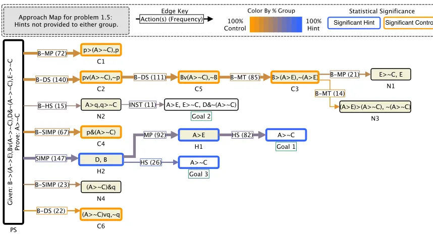
3.4.2 Problem 1.5 . . . 40
3.4.3 Working Backwards and Trailblazing . . . 41
Chapter 4 Exploring Networks of Problem-Solving Interactions . . . 44
4.1 Introduction . . . 44
4.1.1 Previous Work . . . 45
4.2 Modeling Problem Solving. . . 46
4.2.1 Interaction Network . . . 47
4.2.2 Interpretation . . . 49
4.2.3 Network Features . . . 51
4.3 Applications . . . 55
4.3.1 Hint Policies. . . 57
4.3.2 Visualization . . . 57
4.3.3 Graph Mining. . . 58
4.4 Success Stories . . . 59
4.4.1 The Deep Thought Tutor. . . 60
4.4.2 BeadLoom Game . . . 60
4.4.3 iList . . . 61
4.4.4 BOTS . . . 64
4.5 Discussion. . . 65
Chapter 5 Interaction Network Estimation: Predicting Problem-Solving Diver-sity in Interactive Environments. . . . 68
5.1 Introduction . . . 69
5.1.1 Previous Work . . . 70
5.2 Methods and Materials . . . 71
5.2.1 Constructing an Interaction Network . . . 72
5.2.2 Providing Hints . . . 74
5.2.3 Cold Start Problem. . . 75
5.2.4 Good-Turing Network Estimation. . . 75
5.3 Results . . . 77
5.3.1 H1: Prediction of New States. . . 77
5.3.2 H2: Network Coverage . . . 78
5.3.3 H3: Predicting Future Network Size . . . 78
5.3.4 H4: Comparing State Matching Functions. . . 79
5.3.5 H5: Comparing Populations . . . 81
5.3.6 Estimating the effect of filtering . . . 82
5.4 Discussion. . . 83
5.5 Conclusions and Future Work . . . 86
Chapter 6 Conclusions . . . 87
LIST OF TABLES
Table 1.1 Number of students that continued or dropped out of the tutor after L1 7 Table 1.2 The effect sizes of the differences between hint group and control group
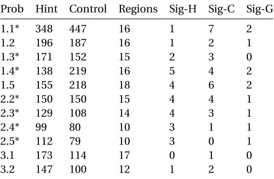
for completion and attempt rates by level. . . 7 Table 3.1 Summary of Approach Maps for 11 Deep Thought tutor problems. An
asterisk (*) indicates problems where the hint group had access to hints. 35 Table 3.2 Detailed information on the regions in the 1.4 Approach Map shown in
Figure 3.1. . . 38 Table 3.3 Number and depth of hints used by the hint group in each region;
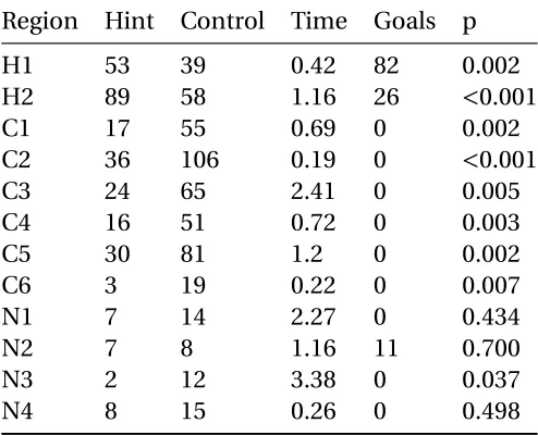
PS=Problem Start . . . 38 Table 3.4 Detailed information on the regions in the 1.5 Approach Map shown in
Figure 3.3. . . 41
Table 4.1 Averages across the datasets, dr is the directed assortativity, r is the undirected assortativity, andS(g)is the scale-free metric. . . 55 Table 4.2 Interaction Networks generated from problems in the 2009 Hint
Fac-tory dataset[SEBC13]. Alpha is the exponent of the fitted power-law distribution, logLik is the log-likelihood of the fit with xmin, KS is the Kolmogorov-Smirnov test statistic (smaller score indicates better fit), p is the p-value of the KS test, values less than 0.05 reject a power-law fit. 56 Table 4.3 Averages across all Interaction Networks generated from problems in the
BOTs(Code and World) and DT(DT1 and DT3). Variables are the same as those in Table 4.2. . . 56 Table 4.4 Example Hint Template which translates the elements of an Action into
4 levels of hints. . . 58 Table 4.5 Actions Available in the BLG . . . 61 Table 4.6 Example Play Sequence . . . 63
LIST OF FIGURES
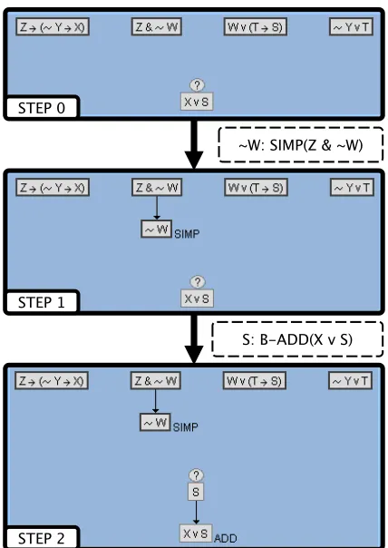
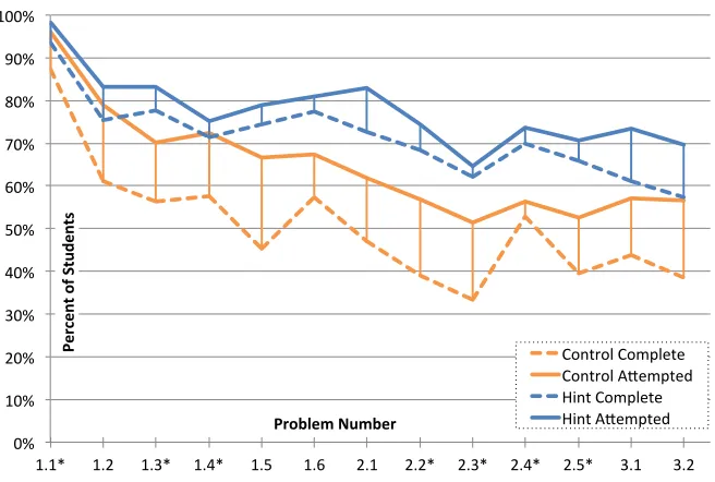
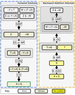
Figure 1.1 This example shows two steps within the Deep Thought tutor. First, the student has selectedZ ∧ ¬W and performed Simplification (SIMP) to derive¬W. Second, the student selectsX ∨Sand performs backward Addition to deriveS. . . 7 Figure 1.2 Attempt and complete rates per level, *indicates a problem where the
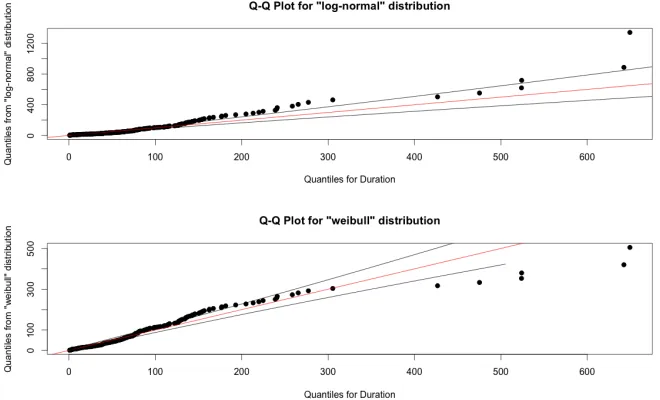
hint group was given access to automatically generated hints. . . 8 Figure 2.1 QQ-Plots for the log-normal and Weibull distributions, the primary
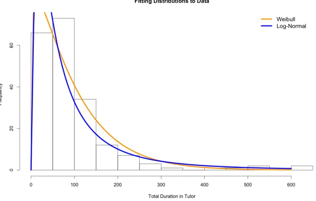
difference appears to be that the Log-normal is sensitive to very small durations, while the Weibull distribution is sensitve to very large dura-tions. . . 20 Figure 2.2 Histogram with density plots for the Weibull and log-normal
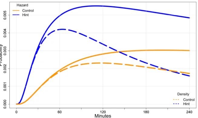
distribu-tions. Both seem to fit reasonably well. . . 21 Figure 2.3 The probability density functions, represented by the dashed lines,
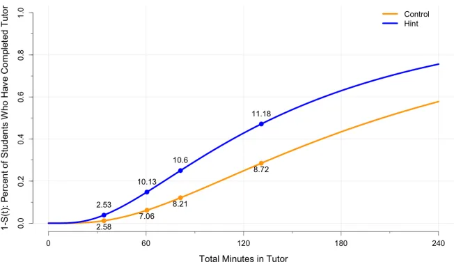
provide the probability of observing tutor completion at a specific time. The hazard functions, the solid lines, are the probability of observing tutor completion at a specific time, given that it has not occurred yet. The probability of completion grows rapidly before becoming stable and eventually decreasing. . . 25 Figure 2.4 The percent of students who have completed the tutor over time. We
have added points with the mean tutor score (max of 13) to each curve at the 20%, 40%, 60%, and 80% quantiles of total duration. . . 26 Figure 3.1 The Approach Map for problem 1.4. Edges and vertexes can be read
as the number of students who performed action(s) to derive propo-sition(s). Three main approaches are revealed, with the hint group strongly preferring to work the problem forwards. The control group often attempts to solve the problem by wards with addition, there are no goals along this path. More detail is given in Table 3.2. . . 37 Figure 3.2 The most common attempt paths for each of the main approaches in
the approach map for problem 1.4 (figure 3.1.) The highlighted nodes represent unjustified propositions. . . 39 Figure 3.3 Even in the absence of the automatically generated hints, the hint group
Figure 4.1 An example Interaction Network. The vertices represent tutor states, edges represent actions that go from state to state, edge thickness is weighted by frequency, goal states are green, and vertices with high attrition rates have red boarders. . . 50 Figure 4.2 Example of a problem-space. The black states represent parts of the
problem space are are not visited by human walkers. The blue and orange states represent the states observed from two different popula-tions of human walkers. . . 51 Figure 4.3 Interesting problems must have meaningful choices. No matter what
action the student takes they move from the start state (white) toward the goal state (green), the rule-using problems we want to focus on allow divergence. . . 52 Figure 4.4 The vertices represent a convexity, or ’bubble’, which is a region within
an Interaction Network where the problem expands from one state and then later converges to a single state. If there are multiple paths to get to the goals, and they can cross over, these types of structures should exist in the network. . . 52 Figure 4.5 Observed networks rarely have complete bubbles, the grey edges and
vertices represent places that the either we have yet to observe a student visiting or that it cannot be reached. . . 52 Figure 4.6 An example of an assortative network (right) where vertices connect
to vertices with similar degree, and a dissortative network (left) where vertices share edges with vertices of different degree. . . 56 Figure 4.7 The in-degree vs. out-degree ratio can reveal information about the
complexity of problems. Degree assortativity is the tendency for vertices to share edges with vertices with a similar degree. . . 57 Figure 4.8 The Approach Map for problem 2.4. Edges and vertices can be read
as the number of students who performed action(s) to derive proposi-tion(s). Several approaches are revealed, with the hint group strongly preferring to work the problem forwards. The control group is more likely to try approaches from which there are no goal paths. . . 59 Figure 4.9 Example problem state in the Deep Thought logic tutor. . . 62 Figure 4.10 The BeadLoom Game Interface: the goal of the game is to create the
pattern on the left in as few moves as possible. Here the player has started by using the rectangle tool to create the first part of the pattern. Next a player might choose the color blue, and draw a blue rectangle, by entering the coordinates in the panel in the bottom right. . . 62 Figure 4.11 An example problem in BOTS. The goal is to use commands to move the
Figure 5.1 Example of state to state transitions within the Deep Thought (DT1) propositional logic tutoring system. . . 73 Figure 5.2 The growth of new states as new students are added for each problem,
for each dataset. . . 78 Figure 5.3 The average absolute error between the estimated number of new states
and the observed new states over the number of students for all prob-lems in each of the four datasets.P0accurately predicts the observed
values after roughly 10 students, rarely being off by more than one after that. . . 79 Figure 5.4 For the hintable states, the average difference between the estimated
number of new states and the observed new states over the number of students for all problems in each of the four datasets.P0accurately
predicts the observed values after roughly 10 students, rarely being off by more than one after that. . . 80 Figure 5.5 The estimated network coverage IC for each of the 5 datasets, note
the poor coverage for the BOTS-C dataset. The BOTS-W state is more general and has the much higher coverage. . . 81 Figure 5.6 An image of the main gameplay interface for BOTS. The left hand side
of the screen shows the user’s program, used to derive code states. The right-hand side shows the game world, where the program output determines the world states. . . 82 Figure 5.7 For the hintable network: the estimated network coverageIC for each
of the 5 datasets. Even the lowest performing hint network BOTS-C reaches roughly 70% coverage by 100 students. . . 83 Figure 5.8 Prediction of total final number of states, as observed number of states
increases. Note that for smallt, the estimate is very high (up to 300% over prediction), but becomes fairly accurate after roughly 20% of the sample is measured. . . 84 Figure 5.9 Prediction of total final number of goal states, as observed number of
states increases. Note that for smallt, the estimate is very high, but becomes an underestimate ast increases.P0can predict the number
Chapter 1
Introduction
The high level goal of this work is to use data-driven methods to understand how people solve problems within problem solving environments, as well as to evaluate the differences in the ways that people solve problems, and finally to use this understanding to change problem-solving behavior.
In this work we take a Educational Data Science approach, using a variety of analytic methods and techniques on user log data collected from educational computer programs. Data Science is the extraction of knowledge and insight from large volumes of structured and unstructured data[Dha13]. This is a relatively new field which combines data min-ing, predictive analytics, exploratory data analysis, data visualization, inferential statistics, as well as concepts such as big data and scalability. Educational Data Mining is also an emerging discipline, which focuses on deriving knowledge about human learning and educational settings from the increasingly large-scale data collected from learning environ-ments[Soc14].
The primary contributions of this work are new methods to explore and evaluate:1) the effects of automatically generated hints on student behavior (tutor performance and learn-ing);2) duration data in problem solving environments;3) higher-level approaches to problems;4) differences in problem solving approaches between groups; and5) how fea-tures of a complex network can be used to characterize user interactions in computer-based tutors.
1.1
Motivation
One-to-one tutoring has a dramatic effect on student learning. Bloom famously found that students given one-to-one tutoring, by human tutors expert in both the content and in ped-agogy, performed two standard deviations better than students given traditional instruction [Blo84]. This effect brought the average student in the tutor-group to above 98% of the control group[Blo84]in terms of performance. It also greatly lowered the variance within the tutor-group, meaning that there were less individual performance differences within the same class, which means that students that would have otherwise been considered low performerswere now performing the same as their peers[Blo84]. However, the cost of one-to-one tutoring for all of the students is too high, and Bloom challenged researchers to find methods of group instruction that are as effective as one-to-one tutoring, also known as the 2-Sigma Problem[Blo84].
The market for supplementary education is estimated to be about $13.1 Billion USD in 2012[Adv12]. One example of the cost of supplemental educational services (SES), as part of a provision of No Child Left Behind law, sees averages hourly rates of $46 USD[BSD07], and this is not necessarily one-to-one tutoring. The high cost associated with private tutoring and other educational materials clearly raises concerns about equal access based on family income. In Korea, where the private tutoring market is even larger at $19 billion USD in 2008, Choi found that family income affected student access to tutoring as well as academic performance[Cho12].
to continue getting better. Koedinger et al. showed that the PUMP algebra tutor improved student performance on standardized tests by 15%[KAH+97]. Corbett argued that intelligent tutors have already closed this gap, and have perhaps surpassed human tutors[Cor01] given the results of a meta-analysis of several successful tutoring systems.
However, the development of intelligent tutoring systems is also expensive, one esti-mate is that each hour or tutoring content requires as much as 100–1000 hours of work [Mur99]. The work involved also requires experts in the fields such as cognitive psychology, educational psychology, computer science, cognitive science, and instructional design. Another potential weakness is that intelligent tutoring systems and other computer-aided instructional environments make it difficult for instructors to track how their students are solving problems within the system, this type of detachment can lead to a decreased sense of control and could effect adoption of the tutor[Sel07]. However, once the system is developed the implication is that personalized tutoring can be widely disseminated and made available at reasonable costs[Woo10, Cor01].
The large educational benefits of private tutoring can be matched by intelligent tutoring systems and these computer-based tutors can make the wide scale adaptation of personal-ized education economically viable. However, intelligent tutors are difficult and expensive to design and develop. The National Academy of Engineering citedPersonalized Learning as one of the 14 grand challenges for engineering[oE14].
The Cognitive Tutor Authoring Tools (CTAT) attempted to help improve the efficiency of tutor development by providing a set of authoring tools, as well as simplifying the tutor creation process[AMSK06]. CTAT was able to improve development time by 1.4 to 2 times [AMSK06]. However, this is still a significant amount of time and still requires the use of experts across many fields. CTAT also places constraints on the tools and systems which the authors must use and is designed for building new tutors, but does not provide support for already existing instructional tools.
1.2
Previous Work
In 2008 Barnes and Stamper approached the tutor development problem by taking a computer-aided instructional program and using previously collected student data to automatically generate the basic features of an intelligent tutoring program[BS08a]. Barnes and Stamper used a machine learning approach and modeled previous student work as a Markov Decision Process (MDP); they then used this MDP to create a best next-step policy, which allowed them to provide a new student with a next-step hint[BS10]. A pilot study using this technique showed that students used the system, and that the automatic method of providing hints was able to provide hints 91% of the time they were requested[SBLC08b]. Barnes and Stamper also found that visualization of the MDPs themselves revealed sur-prising insights into how the student’s solved the problems[BS08a]. The MDP method of generating next-step hints, also called Hint Factory, has been applied across domains (linked list tutor, logic tutor, and programming game)[FDEO+09, PIHB14, EJBB13], and been shown to increase student retention in tutors[SEBC13].
In section 1.2.2 we summarize the results from Stamper, Eagle, and Barnes’ 2009 study on automatically generated hints[SEBC13]. In Chapter 2 we provide a followup analysis on student time-in-tutor vs. completion rates and show that the the automatically generated hints reduce the time needed to complete the tutor by almost 50/
The Hint Factory approach provided feedback in an environment without high levels of problem scaffolding, a common feature of most intelligent tutoring systems[Van06]. The typical tutoring system is designed by carefully breaking down the problem domain into knowledge components, basic units of knowledge, and scaffolding the problems such that each step of the problem uses only a single knowledge component[Van06]. Doing this allows the researcher to develop student models using systems such as ACT-R (as seen in the early LISP tutors,)[ACKP95]or later generalizations such as Bayesian Knowledge Tracing[CA94]. However, it is often necessary to strongly restrict the presentation of the problems to use these techniques, which makes it difficult to incorporate in already existing systems.
expands on the results, and offers a more detailed view into how the automatically generated hints affected student’s time within the tutor.
Eagle and Barnes abstracted the MDP domain model into a complex network repre-sentation of the student-tutor interactions called an Interaction Network[EJB12]. These networks worked well as visualizations of student work within tutors and Johnson et al. suc-cessfully created a visualization toolInVisspecifically to aid instructors in understanding student-tutor interaction data[JEB13]. Interaction Networks have been used for the devel-opment of data-driven mastery learning[EB12]. One of the contributions of this work is that analysis of the Interaction Networks with network mining techniques allowed us to derive useful sub-regions which represented diverse student approaches to solving problems [EB14a](see Chapter 3).
Chapter 4 presents work on furthering the understanding of Interaction Networks and their interpretation. Specifically, we address treating the Interaction Networks as sam-ples from a population. We also explore the types of educational environments where Interaction Networks work best by exploring the overall shape and distribution of states and connectivity within the network. We present evidence that Interaction Networks are scale-free networks, that is, the vertex connectivity frequency distribution follows a power-law. We also make further use of network invariants such as assortativity to describe the high-level characteristics of the network. We argue that these properties allow Interac-tion Networks to work across a wide variety of instrucInterac-tional environments, even when the potential problem-space might seem intractable.
1.2.1
The Deep Thought Logic Tutor
In Deep Thought propositional logic tutor problems, students apply logic rules to prove a given conclusion using a given set of premises. Deep Thought allows students to work both forward and backwards to solve logic problems[Cro00]. Working backwards allows a student to propose ways the conclusion could be reached. For example, given the conclusionB, the student could propose thatB was derived using Modus Ponens (MP) on two new, unjustified (i.e. not yet proven) propositions:A→B,A. This is like a conditional proof in that, if the student can justifyA→BandA, then the proof is solved. At any time, the student can work backwards from any unjustified components (marked with a ?), or forwards from any derived statements or the premises. Figure 1.1 contains an example of working forwards and backwards with in Deep Thought.
1.2.2
2009 Deep Thought Study
This section provides detail on an important dataset for this document. The author designed the second half of this study, and performed the evaluation. In 2013, Stamper, Eagle, and Barnes studied the effect of data-driven hints[SEBC13]using the Spring and Fall 2009 Deep Thought propositional logic tutor dataset[SEBC11]. Data was collected from six 2009 deductive logic courses, taught by three professors. Each instructor taught one class using Deep Thought with automatically-generated hints on half of the problems (hint group, n=105) and one without access to hints on any problems (control, n=98). Students from the 6 sections were assigned 13 logic proofs in Deep Thought as a series of three graded homework assignments, with problems L1: 1.1-1.6, L2: 2.1-2.5, and L3: 3.1-3.2.
Table 1.1 shows retention information for each group after level L1; aχ2 test of the
relationship between group and dropout producedχ2(1) =11.05, which was statistically
significant atp=0.001. The hint group completed more problems, with the effect sizes for these differences shown in Table 1.2. Stamper et al. found that the odds of a student in the control group dropping out of the tutor were 3.6 times more likely when compared to the group provided with automatically generated hints[SEBC13].
Figure 1.1: This example shows two steps within the Deep Thought tutor. First, the student has selectedZ ∧ ¬W and performed Simplification (SIMP) to derive¬W. Second, the student selectsX ∨Sand performs backward Addition to deriveS.
Table 1.1: Number of students that continued or dropped out of the tutor after L1
Group Total # Continued # Dropped % Dropped
Hint 105 95 10 9%
Control 98 71 27 28%
Total 203 166 37 18%
Table 1.2: The effect sizes of the differences between hint group and control group for completion and attempt rates by level.
L1 L2 L3
Note that, after problem 1.4, the differences in attempt rates and completion rates seem to diverge between the groups.
0% 10% 20% 30% 40% 50% 60% 70% 80% 90% 100%
1.1* 1.2 1.3* 1.4* 1.5 1.6 2.1 2.2* 2.3* 2.4* 2.5* 3.1 3.2
Percen
t o
f S
tu
den
ts
Problem Number
Control Complete Control A9empted Hint Complete Hint A9empted
Figure 1.2: Attempt and complete rates per level, *indicates a problem where the hint group was given access to automatically generated hints.
1.3
Organization
Below we have listed each chapter and its problem statement, research questions, our approach, and our conclusions.
1.3.1
Chapter 2: Effects of Automatically Generated Next-Step Hints on
Student Time-in-Tutor and Retention
Problem
Intelligent tutoring systems have sizable effects on student learning efficiency — spending less time to achieve equal or better performance. In a classic example, students who used the LISP tutor spent 30% less time and performed 43% better on posttests when compared to a self-study condition[AR85]. While this result is quite famous, few papers have focused on differences between tutor interventions in terms of the total time needed by students to complete the tutor. In many studies of intelligent tutoring systems, time is simply held constant for two groups, and efficiency then boils down to comparing the number of problems each group could solve in the given time and the results of posttest measures. However, it is not clear how to factor students who were not able to complete the tutor into this analysis. Typical time duration distributions violate the normality assumptions of many statistical tests and measures of central tendency. Anderson, Corbett, Koedinger, and Pelletier used mean duration data to compare differences between groups of students with and without intelligent feedback in the LISP tutor[ACKP95]. The authors state that the mean times (for the control group) are underestimates, as many students in the control (no-feedback group) did not complete all assignments. In other words, if the control group persisted, the time they took to complete tasks would have been longer than the observed durations for the few high-performing students who were able to persist without feedback.
Different dropout rates between experimental groups can cause attrition bias[MH07], where groups completing the study are selected due to achievement levels; this self-selection causes the sample to become different than the target population and hampers the study’s generalizability[MEHB97]. When dropout exists, more complex analyses are needed to study learning efficiency; not only are results suspect for generalization purposes, but the data itself contains missing values because of high dropout rates.
Research Questions
Approach
We investigate data from a prior study of the Deep Thought logic tutor comparing versions with and without hints. Stamper et al. found that the odds of a student in the control group dropping out of the tutor after the first six problems were over 3.6 times higher when compared to the group provided with (data-driven and automatically generated) hints [SEBC13]. Students given access to hints also had better tutor performance, as well as higher overall course scores. However, comparison of duration means showed no differences in overall time spent in the Deep Thought logic tutor between the hint and control groups. This is likely because this comparison does not take into account student dropout. In this study, we applied survival analysis to data from Stamper et al.’s study to more fully explore the impact of hints on performance, duration, and dropout.
Our exploration of tutor efficiency has three important elements: performance (tutor completion percentage), duration (total time spent interacting with the tutor), and dropout (whether stopped before completion). Dropout can easily confound the results of duration and performance. By modeling tutor data with high dropout rates using survival analysis, we hypothesize that we can build a more detailed understanding of tutor efficiency and explain differences between groups in an educational intervention.
Contribution
the tutor - equal to the amount of time spent in the tutor by the hint group. The difference is tutor efficiency: students in the hint group performed more efficiently, and were therefore able to complete the tutor, while the control group spent a similar amount of time but was less likely to be able to finish. This is a much richer understanding of the differences in effects between the two groups than traditional methods provide. The survival function also allows us to make predictions on how much time is needed for tutor completion, both for teacher planning and student feedback. These results suggest that survival analysis is a powerful toolbox for investigating the impact of interventions on learning efficiency while accounting for performance, duration, and dropout.
1.3.2
Chapter 3: Exploring Differences in Problem Solving with
Data-Driven Approach Maps
The primary contributions of this chapter are new methods to explore and evaluate higher-level approaches to problems and differences in problem solving approaches between groups.
Problem
Research Questions
In what way does the availability of automatically generated next-step hints effect the way that students solve problems within the tutor? How can we get both a qualitative and quantitative measure of the differences between two groups in terms of how they approach a problem? Can we break the network up into high-level regions, which can summarize the different approaches to a problem? Do the differences in problem-solving persist to problems even when each group is not given access to next-step hints?
Approach
By mapping Deep Thought transactional data into an Interaction Network, and applying graph mining to derive regions based on the structure of this network, we develop a new Approach Map that illustrates the approaches that groups of students take in solving logic problems. We built Approach Maps for all 13 problems in the tutor, and illustrate a detailed analysis of two of these maps to explore the differences in problem solving between the hint and control groups. We use a two-tailed chi-squared test to look for differences between the hint and control groups in how they visit regions in the Approach Map. The null hypothesis is that there is no difference in the frequency of entering a particular region between attempts in the hint group and the control group. The alternative hypothesis is that the groups enter regions with different than expected frequency. We use Bonferroni correction [Sha95]to compensate for the number of tests that we run. We then compare between-group approaches to problems in which one between-group had hints and the other did not, as well as problems in which neither group was given access to hints.
Contribution
Approach Maps annotated with frequencies of visits by two groups to identify regions where a particular study group was over-represented allowed us to examine the approaches each group took to solving each proof. As we predicted, the automatically generated hints seemed to direct the students in the hint group down a common path, and we were able to detect this with the Approach Maps. Interestingly, even in problems where neither group had hints, the hint group still showed a preference for better approaches, providing some evidence for a persistent effect of the hints. Analyzing Approach Maps also facilitated an-other important discovery that control group tended enter and remain in unproductive (or buggy) regions. These observed differences help explain how the automatically-generated hints produced the difference in tutor performance and retention in the 2009 Deep Thought study. Our investigations suggest that the patterns of behavior exhibited by students do result in meaningful regions of the solution attempt search space.
1.3.3
Chapter 4: Exploring Networks of Problem-Solving Interactions
The primary contributions of this chapter are new methods to explore and evaluate how the features of a complex network can be used to characterize user interactions in computer-based tutors.Problem
Problem solving is an important skill across many fields, including science, technology, engineering, and math (STEM). Working open-ended problems may encourage learning in higher ’levels’ of cognitive domains[Blo56]. We have developed Interaction Networks to represent student problem solving in educational environments. In this chapter we explore the properties of Interaction Networks and the types of educational environments in which they work best.
Research Questions
Approach
We explore our theory on what types of problem solving environments Interaction Networks are best suited for. We look into complex network metrics of degree distribution to explore how network connectivity is distributed. We also explore the self similarity, or scale-free, nature of Interaction Networks. We compare results across data from a logic tutor, as well as a educational game for teaching programming.
Contribution
In this chapter we explore tutor Interaction Networks, empirical samples of student-walks though a problem-space modeled as a complex network. Interaction Networks were designed specifically for tutors with problem-solving tasks in which there are many goals and many paths to those goals, and that the user moves along those paths by using a set of actions. We explore Interaction Networks from multiple datasets and find that they exhibit scale-free properties. We find that Interaction Networks from different tutors share similarities in scale-free metrics and find that global and local vertex degree assortativity provide insight into the nature of the problem solving environments.
We present success stories from a variety of tutoring systems and argue that Interaction Networks are useful for a wide variety of problem solving instructional environments, even when the potential problem-space might look to be intractable. The scale-free properties of the network make it possible to discover the important regions of a network even with a small sample of student data. We expect that Interaction Networks are a good representation for describing a large amount of student data; provide a common language for performing cross tutor evaluation of problem solving environments; and that the intuitive nature of the model helps convey results from the data in a way that is interpretable for both research and instructor.
1.3.4
Chapter 5: Interaction Network Estimation: Predicting
Problem-Solving Diversity in Interactive Environments.
Problem
Data-driven methods to provide automatic hints have the potential to substantially re-duce the cost associated with developing tutors with personalized feedback. Modeling the student-tutor interactions as a complex network provides a platform for researchers to automatically generate next step hints. AnInteraction Networkis a complex network representation of all observed student and tutor interactions for a given problem in a game or tutoring system. In addition to their usefulness for automatically generating hints, In-teraction Networks can provide an overview of student problem-solving approaches for a given problem.
Data-driven approaches cannot reliably produce feedback until sufficient data has been collected, a problem often referred to as the Cold Start problem. The precise amount of data needed varies by problem and environment. However, some properties of Interaction Networks allow us to estimate how much data is needed. Eagle et al. explored the structure of these student Interaction Networks and argued that networks could be interpreted as an empirical sample of student problem solving[EHIB15]. Students employing similar problem-solving approaches will explore overlapping areas of the Interaction Network. The more similar a group of students is, the smaller the overall explored area of the Interaction Network will ultimately be. Since we expect different populations of students to have different Interaction Networks, and different domains to require varying amounts of student data before feedback can be given, good metrics for the current and predicted quality of Interaction Networks are important.
Research Questions
How much data is needed to provide hints for a new problem? How much do different populations of students overlap in their solution attempts? How can we compare different state representations?
Proposed Approach
by Alan Turing and his assistant I. J. Good for use in cryptography efforts during World War II. We will adapt this method for observed and unobserved tutor states.
Contribution
We have adapted Good-Turing frequency estimation for use with networks built from student-tutor interactions. We found that the estimator for the missing proportion of the networkP0was accurate in predicting the number of new states discovered with new data.
We also found that we could accurately measure network coverage withIC for both the
Chapter 2
Survival Analysis on Duration Data in
Intelligent Tutors
Effects such as student dropout and the non-normal distribution of duration data confound the exploration of tutor efficiency, time-in-tutor vs. tutor performance, in intelligent tutors. We use an accelerated failure time (AFT) model to analyze the effects of using automatically generated hints in Deep Thought, a propositional logic tutor. AFT is a branch of survival analysis, a statistical technique designed for measuring time-to-event data and account for participant attrition. We found that students provided with automatically generated hints were able to complete the tutor in about half the time taken by students who were not provided hints. We compare the results of survival analysis with a standard between-groups mean comparison and show how failing to take student dropout into account could lead to incorrect conclusions. We demonstrate that survival analysis is applicable to duration data collected from intelligent tutors and is particularly useful when a study experiences participant attrition.
2.1
Introduction
to complete the tutor. In many studies of intelligent tutoring systems, time is simply held constant for two groups, and efficiency then boils down to comparing the number of problems each group could solve in the given time and the results of posttest measures. However, it is not clear how to factor students who were not able to complete the tutor into this analysis. In this chapter, we explore tutor efficiency in terms of time and performance, while taking studentdropout(ceasing to interact with the tutor before completion) into account.
College students often use computer-based tools to complete homework assignments, but no specific time limits apply. Typical time duration distributions violate the normality assumptions of many statistical tests and measures of central tendency. Anderson, Corbett, Koedinger, and Pelletier used mean duration data to compare differences between groups of students with and without intelligent feedback in the LISP tutor[ACKP95]. The authors state that the mean times (for the control group) are underestimates, as many students in the control (no-feedback group) did not complete all assignments. In other words, if the control group persisted, the time they took to complete tasks would have been longer than the observed durations for the few high-performing students who were able to persist without feedback. This study illustrates how dropout can obscure the true impact of an intervention.
Our exploration of tutor efficiency has three important elements: performance (tutor completion percentage), duration (total time spent interacting with the tutor), and dropout (whether stopped before completion). Dropout can easily confound the results of duration and performance. Different dropout rates between experimental groups can cause attrition bias[MH07], where groups completing the study are self-selected due to achievement levels; this self-selection causes the sample to become different than the target population and hampers the study’s generalizability[MEHB97]. When dropout exists, more complex analyses are needed to study learning efficiency; not only are results suspect for generaliza-tion purposes, but the data itself contains missing values because of high dropout rates. By modeling tutor data with high dropout rates using survival analysis, we hypothesize that we can build a more detailed understanding of tutor efficiency and explain differences between groups in an educational intervention.
times higher when compared to the group provided with (data-driven and automatically generated) hints[SEBC13]. Students given access to hints also had better tutor performance, as well as higher overall course scores. However, comparison of duration means showed no differences in overall time spent in the Deep Thought logic tutor between the hint and control groups. This is likely because this comparison does not take into account student dropout. In this study, we applied survival analysis to data from Stamper et al.’s study to more fully explore the impact of hints on performance, duration, and dropout. We hypothesize that students given access to hints in the Deep Thought logic tutor, spend less time in tutor while also performing better than students without hints. In other words, the tutor efficiency for Deep Thought with hints is higher than that for they system without hints. We found that students given automatically generated hints take 55% of the time that students in the control needed to complete the tutor.
2.1.1
Methods and Materials
We perform our experiments on the Spring and Fall 2009 Deep Thought propositional logic tutor[Cro99]dataset as analyzed by Stamper, Eagle, and Barnes in 2011[SEBC11]. Data was collected from six deductive logic courses, taught by three professors. Each instructor taught one class using Deep Thought with automatically-generated hints available (hint group) and one without any additional feedback (control). The dataset includes 105 students in the Hint group and 98 students in the Control group. In Deep Thought, students choose the amount of time they spend using the online tutor; however, they were graded on the completion of 13 specific proofs.
The variables we use for this study are:
Group a two level factor (Hint, Control) depicting the student’s experimental condition
ProblemDuration the sum of the time taken over all steps in a problem until 1st completed (max 3min per step)
Duration the sum of problem durations over all 13 problems
Performance a number between 0–13 representing the number of proofs solved by the student
Figure 2.1: QQ-Plots for the log-normal and Weibull distributions, the primary difference appears to be that the Log-normal is sensitive to very small durations, while the Weibull distribution is sensitve to very large durations.
Duration data often falls into a set of known distributions[BM11] [ME98]. Q-Q plots (figure 2.1) and histogram/density plots (figure 2.2) allowed us to narrow the possible distributions down to log-normal[CS88]or Weibull[W+51]. The primary difference appears to be that the log-normal does not fit well to early dropout (small durations), while Weibull does not fit as well for extremely long durations.
2.1.2
Survival Analysis
Survival analysis is a series of statistical techniques that deal with the modeling of “time to event” data[HLM08]. Survival analysis, also known as reliability analysis or duration analysis in economics, is named for its start as a method to measure survival after applying a medical intervention.
Survival analysis includes techniques for unknown values, non-parametric data, log-normal and Weibull probability distributions, and between-groups testing. We use the survival package for R[The14]to perform our analysis of learning efficiency, where the event for survival analysis is tutor completion.
Figure 2.2: Histogram with density plots for the Weibull and log-normal distributions. Both seem to fit reasonably well.
when participant data is lost before tutor completion, while left censoring would be when completion time is known but start time is not. For our data, the duration for students who drop out, or stop using the tutor is right censored, since we know the start time but do not know how long it would have taken the student to complete the tutor. For example, a student who has completed 5 problems but then quits is considered right censored as we do not know how long it would have taken the student to complete all 13 problems.
The survival function is defined as:
S(t) =P r(E >t) =1−F(t) (2.1)
wheret is the time in question,E is the time of the event (tutor completion),P r is proba-bility, F(t) is the duration distribution. This function gives the probability that the time of the tutor completion event,E, is later thant. That is, the probability that the student has not completed the tutor.
The duration distribution function, which is found via the cumulative distribution functionc d f(t), is the probability of observing a problem completion timeE less than or equal to some time
The derivative of F(t) is the probability density function (p d f ) of the duration distribu-tion,
f(t)P r(E =t) =F0(t) = d
d tF(t) =p d f (t), (2.3) which provides us with the probability of observing a single tutor completion timeE at some timet. The hazard function, which tells us the instantaneous completion rate at time t, is:
λ(t) = lim
d t→0
P r(t ≤E <t +d t|E ≥t)
d t =
f(t) S(t) =
p d f(t)
1−c d f(t). (2.4) This is the probability of the event occurring at time t given that the event has not yet occurred.
There are two models we consider for measuring effects of covariates: the accelerated failure time (AFT) model and the Cox proportional hazards model. AFT assumes that the effect results in one group that completes the tutor more quickly, while the Cox proportional hazards model assumes that the tutor completion rate for one group is a constant multiple of that for the other. We have chosen the AFT model, which assumes that the effect of the covariates,θ, is to accelerate the time to tutor completion by some constant factor[TP00].
S(t|θ) =S(θt) (2.5)
The AFT model assumptions fit with our hypothesis that hints shorten the time it takes to finish the tutor. In addition, it is easy to interpretθ as a direct modifier to tutor completion time, and AFT facilitates using data from log-normal and Weibull distributions.
2.2
Results
p d f(t) = p 1 2πσte
−[ln(2tσ)−µ2]2,c d f(t) =Φ(lnpt−µ
2σ2 ). (2.6)
whereΦ(x) is the cumulative distribution function (cdf ) of the standard normal distribution. Note that we use ln(t)when usingΦ, we can do this thanks to the assumption that the log of the duration data shows a normal distribution.
The AFT model was statistically significantχ2=9.21 on 1 degree of freedom,p=0.0024,
n=202, the coefficients of the model had the intercept (mean) as 5.655, the effect of Hint
θ as−.599, and theS D (scale) as 0.948. The effect of hints ise−.599=0.55; this means that it
takes the Hint group 55% of the time it takes the control group to solve all 13 tutor problems. We have plotted the inverse of the survival curve in figure 2.4.
Figure 2.3 shows the hazard function for the duration data, in other words, the instanta-neous completion rate for each of the groups. It also shows the probability density function for the completion rate. Overall, these plots give us a good overview of the shape of the duration data, showing that the probable total duration for students in the control group, if they were to complete the tutor, would be much longer than that for students in the hint group. One concrete measure of this is illustrated by the median of the survival function, the location where 50% of people have completed the tutor. The median is found byeµ, which ise5.65=284.29 for the control group ande5.65−.599=156.18 for the hint group. Comparing
these medians illustrates again the considerable difference in duration, or time to tutor completion, between the groups.
To illustrate the impact of dropout, we compare the results of survival analysis to a more traditional between-groups testing method. To explore differences in overall time in tutor between the two groups, we subjected the total elapsed time on all 13 problems to a 2-tailed Student’s t-test. The total time in tutor between the hint group (M=86.05,S D =69.80) and the control group (M =122.95,S D=122.94) was not significant,t(200) =−1.34,p=0.183.
However, since we know the data isn’t from a normal distribution, we can improve on this accuracy by using a data transformation. To normalize the data, we use a logarithmic transformation (common log, base 10) to make the data more symmetric and homoscedas-tic. We subjected the log-transformed data to a 2-tailed Student t-test. The difference in the logs of duration between the hint group (M =8.20,S D=1.02) and the control group (M =8.17,S D =1.21) was not significant,t(200) =.168,p=0.867. The ratio of the duration between groups is calculated by taking the difference between the means of the groups, since lg(x)−lg(y) =lg(xy). The confidence interval from the log-data estimates the difference between the population means of log transformed data. Therefore, the anti-logarithms of the confidence interval provide the confidence interval for the ratio. The anti-log of the log-transformed means provides us with the geometric mean, the anti-log of the trans-formed standard deviation is not interpretable. However, we can use the anti-log of the confidence intervals. The most useful statistic we can derive is the difference ratio, and its corresponding confidence intervals. A difference ratio of 0.026 between the means of the logged data equates to 10.026=1.06 with a 95% confidence interval ofC I (0.52, 2.19).
2.3
Discussion
The results of the survival analysis allow us to reveal striking differences between the hint and control groups in terms of the time needed to complete the tutor. Students in the hint group complete the tutor in just over half the time needed for students in the control group. It is interesting that the control group and the hint group do not haveobserveddifferences in overall tutor time; in other words - students in the control group don’t generally complete the tutor, so we can’t observe that they would take twice as long. It is likely that, given the nature of the online access tutor, students are only willing to spend a certain amount of time on this homework assignment. This can explain the observations of differences in tutor progress observed at different times in figure 2.4.
Figure 2.3: The probability density functions, represented by the dashed lines, provide the probability of observing tutor completion at a specific time. The hazard functions, the solid lines, are the probability of observing tutor completion at a specific time, given that it has not occurred yet. The probability of completion grows rapidly before becoming stable and eventually decreasing.
time) is 284 minutes for the control group and 156 minutes for the hint group. Dividing this by the number of problems in the tutor (13) gives us an estimate of efficiency, since it gives a time per problem needed for solution. The control group is therefore spending about 21 minutes per problem on average, while the hint group is spending an average of 12 minutes per problem. Although this estimate is derived using curves to estimate the (unknown) completion time for the control group, it does in fact fit with the observed data in the first several problems, before significant dropout in the control group occurred. Given these very different rates, we can see that the control group could be discouraged by solving less than 3 problems in an hour, while the hint group could solve 5 in the same amount of time. We were in fact surprised, after realizing these estimates, that students in the control group did not drop out sooner than they did!
Figure 2.4: The percent of students who have completed the tutor over time. We have added points with the mean tutor score (max of 13) to each curve at the 20%, 40%, 60%, and 80% quantiles of total duration.
et al.[BLJS01]defined the efficiency of a tutor, for how the student perceives it, as the “belief or judgement that information can be accessed without wasting time or effort.” Scanlon and Issroff[SI05]posit that computer-based instruction can conflict with the student’s perceptions of division of labour within learning context. In other words, students using computer-based instruction must be more self-directed and manage their own learning. The feedback provided by the tutor with hints might have helped students in the hint group feel more directed, while also helping them when they were stuck. This could have led to improved student perceptions of efficiency.
be allocated in schools for students to use a tutor. We are considering using these estimates to proactively indicate to students when they might need to seek outside help. For example, if a student has taken more than the estimated time for half of students in their group to complete the tutor, we could suggest they speak to a teaching assistant.
2.4
Conclusions
Chapter 3
Exploring Differences in Problem Solving
with Data-Driven Approach Maps
Understanding the differences in problem solving behavior between groups of students is quite challenging. We have mined the structure of interaction traces to discover different approaches to solving logic problems. In a prior study, significant differences in perfor-mance and tutor retention were found between two groups of students, one group with access to hints, and one without. The Approach Maps we have derived help us discover differences in how students in each group explore the possible solution space for each problem. We summarize our findings across several logic problems, and present in-depth Approach analyses for two logic problems that seem to influence future performance in the tutor for each group. Our results show that the students in the hint group approach the two problems in statistically and practically different ways, when compared to the control group. Our data-driven approach maps offer a novel way to compare behaviors between groups, while providing insight into the ways students solve problems.
3.1
Introduction
Eagle, and Barnes showed that students with access to hints in the Deep Thought logic tutor spent 38% less time per problem and completed 19% more problems than the control group[EB14b]. In another study on the same data, Stamper, Eagle, and Barnes showed that students without hints were 3.6 times more likely to drop out and discontinue using the tutor[SEBC13].
Procedural problem solving is an important skill in STEM (science, technology, en-gineering, and math) fields. Open-ended procedural problem solving, where steps are well-defined, but can be combined in many ways, can encourage higher-level learning [Blo56]. However, understanding learning in open-ended problems, particularly when stu-dents choose whether or not to perform them, can be challenging. The Deep Thought tutor allows students to use logic rules in different ways and in different orders to solve 13 logic proof problems for homework. In this paper, we analyze the 2009 Deep Thought data set analyzed by Stamper, Eagle, and Barnes to further understand the differences between the hint and control groups.
The rich interaction data saved by transactional tutor logs offers many avenues to ex-plore and understand student problem solving data, particularly for problems with multiple solutions. By mapping Deep Thought transactional data into an Interaction Network, and applying graph mining to derive regions based on the structure of this network, we develop a new Approach Map that illustrates the approaches that groups of students take in solving logic problems. We built Approach Maps for all 13 problems in the tutor, and illustrate a detailed analysis of two of these maps to explore the differences in problem solving between the hint and control groups.
The Approach Maps for problems 1.4 and 1.5 show that the hint group explored pro-ductive regions of the Interaction Network, while students in the control group were more likely to explore unproductive regions that did not lead to solutions. Problem 1.4 had avail-able hints for the hint group. Even though problem 1.5 has no hints for either group, the Approach Map shows that the two groups still explore the problem space differently, illus-trating that prior access to hints had a lasting effect. The Approach Maps help us discover unproductive regions of the problem-solving space, that we believe contributed to lower retention rates for the control group. In these regions, proactive hints could be used to direct students toward more productive approaches.
the results and illustrates two detailed Approach Maps on problems 1.4 and 1.5. Finally, we discuss the results, conclusions, and future directions for this work.
3.2
Related Work
Although they can be very effective, the construction of intelligent tutors can be costly, requiring content experts and pedagogical experts to work with tutor developers to identify the skills students are applying and the associated feedback to deliver[Mur99]. One way to reduce the costs of building tutoring systems is to build data-driven approaches to generate feedback during tutor problem-solving. Barnes and Stamper built the Hint Factory to use student problem-solving data for automatic hint generation in a propositional logic tutor [BS08a]. Fossati et al. implemented Hint Factory in the iList tutor to teach students about linked lists[FDEO+09]. Evaluation of the automatically generated hints from Hint Factory showed an increase in student performance and retention[SEBC13]; more details about this study are provided in section 1.2.2.
Although individual differences affect the ways that students solve problems[Jon00], it is difficult to examine the overall approaches that groups of students demonstrate during problem-solving. While pre and posttests are useful for measuring the change in behavior before and after an experimental treatment, we are interested in studying not only whether a student can solve a problem, but how they are solving the problem. In this study, we use Interaction Networks of student behaviors to investigate how providing hints affects student problem-solving approaches.
solving problems.
The Girvan-Newman algorithm (GN) was developed to cluster social network graphs using edge betweenness to find communities of people[GN02]. The technique also works in other domains. Wilkinson et al. applied GN in gene networks to find related genes[WH04]. Gleiser et al. used GN to discover essential ingredients of social interactions between jazz musicians[GD03]. We are the first to apply GN to Interaction Networks consisting of problem-solving steps.
In this paper, we mine the interactions from student problem solving data to summarize a large number of student-tutor transaction data into an Approach Map, demonstrating the diverse ways students solve a particular problem. We use Approach Maps to better understand the differences in behavior between two groups, students who were given access to hints, and those who were not, while completing homework in theDeep Thought logic proof tutor.
3.3
Methods
In Section 3.3.1, we describe how we use Deep Thought tutor logs to create an Interaction Network of all the student-tutor interactions within a single problem. We then show how we refine this network intoregionsof densely connected subgraphs (Section 3.3.2) using the Girvan-Newman (GN) algorithm. Finally, in Section 3.3.2 we define how we construct Approach Maps from the GN regions. For both steps in the process, we use the statistical environmentR[R C12], and the complex network research libraryiGraph[CN06].
3.3.1
Constructing an Interaction Network
to STEP2 with actionB−AD D (backwards addition) applied to(X∨S)to derive the new, unjustified statementS.
We use a state matching function to combine identical states, that consist of all the same logic statements, but may have been derived in a different order. This way, the state for a step STEP0, STEP1, or STEP2 in Figure 1.1 is the set of justified and unjustified statements in each screenshot, regardless of the order that each statement was derived. We use an action matching function to combine actions, and preserve the frequency of each observed application.
If we treat the interactions used to create the networks assamplesof observed behavior from a population, we could expect that the Interaction Networks constructed from different populations may have observable differences. However, rather than building two separate Interaction Networks and attempting to compare them, we construct a single network but keep track of the frequencies of visits by the hint and control groups for each state (vertex) and action (edge).
3.3.2
Extracting Regions
We partition the Interaction Network into densely connected subgraphs we callregions using Girvan and Newman’s edge-betweenness clustering algorithm[GN02]and modularity score, a measure of the internal verses external connectedness of the regions[NG04]. We use following algorithm to apply region labels to nodes in a Deep Thought Interaction Network. First, we remove the problem start state and goal states from the Interaction Network IN to createG1. Then, we iteratively remove all edges inG1, in order of edge betweenness.
Edge betweenness (EB) for a particular edgeeis calculated by computing all shortest paths between all pairs of nodes, and counting the number of shortest paths that contain the edge e. At each GN iterationiand graphGi, we find the edge with the highest EB, and call this
bridgebi. We remove the bridgebi from the graphGi, and compute the modularity score
for the resulting graphGi+1. The process is repeated until all edges have been removed.
Then, we assign identifiers to all nodes in the disjoint regions in the intermediate graph Gn with the best modularity score. At the end of this process, we useGn to construct the
Approach Map with nodes for the original start and goal states, and a new node for each region inGn. The Approach Map edges are the edges that connect the start state and goals
Regions represent sets of steps that are highly connected to one another. When a solution attempt is within a region, new actions will stay within the region, or take a bridge edge into another region or goal. If an attempt is in a region with no goal bridges, the student must take a bridge to another region to reach a goal. Therefore, paths on the Approach Map can be interpreted as a high-level approaches to solving the problem. We hypothesize that we can use the Approach Map to discover different problem-solving approaches. In the next section, we investigate Approach Maps for two problems in Deep Thought, after which the hint and control groups diverged in performance.
Approach Map
Here we provide a more detailed description of the algorithm we use to generate an Ap-proach Map from the Interaction Network for a problem after its nodes have been labeled with region identifiers. A regionA(or actiona)dominatesa regionBif every path from the start of the problem toB, must go throughA(ora).
1. Combine all nodes with the same region identifier into a single region node labeled with the identifier, and remove all the edges with the same region identifier.
2. Combine all goal states that are dominated by a single region into a single goal node. 3. Calculate chi-squared to find in-edge frequencies that are different than expected
between the groups (described in more detail below).
4. Combine parallel bridge edges between two regions into complex edges that represent the combination of the actions.
5. Label each region with the post conditions (derived statements) that result from the most frequent in-edge actions.
6. Provide new region identifiers that indicate the significant regions by the group with larger than expected frequency, with a number indicating the order in which the region was formed. For example, the regions the hint group visits more than expected are H1, H2, ..., the regions the control group visits more than expected are C1, C2, ..., and those that are visited as expected by both groups are labeled N1, N2, etc.