Vehicle Distance Detection Using Monocular Vision and Machine Learning

(1)

University of Windsor University of Windsor

Scholarship at UWindsor

Electronic Theses and Dissertations Theses, Dissertations, and Major Papers

11-23-2019

Vehicle Distance Detection Using Monocular Vision and Machine

Learning

Maryam Samir Naguib Girgis Hanna

University of Windsor

Follow this and additional works at: https://scholar.uwindsor.ca/etd

Recommended Citation Recommended Citation

Hanna, Maryam Samir Naguib Girgis, "Vehicle Distance Detection Using Monocular Vision and Machine Learning" (2019). Electronic Theses and Dissertations. 8142.

https://scholar.uwindsor.ca/etd/8142

This online database contains the full-text of PhD dissertations and Masters’ theses of University of Windsor students from 1954 forward. These documents are made available for personal study and research purposes only, in accordance with the Canadian Copyright Act and the Creative Commons license—CC BY-NC-ND (Attribution, Non-Commercial, No Derivative Works). Under this license, works must always be attributed to the copyright holder (original author), cannot be used for any commercial purposes, and may not be altered. Any other use would require the permission of the copyright holder. Students may inquire about withdrawing their dissertation and/or thesis from this database. For additional inquiries, please contact the repository administrator via email

(2)

Vehicle Distance Detection Using Monocular

Vision and Machine Learning

By

Maryam Samir Naguib Girgis Hanna

A Thesis

Submitted to the Faculty of Graduate Studies

through the Department of Electrical and Computer Engineering

in Partial Fulfillment of the Requirements for

the Degree of Master of Applied Science

at the University of Windsor

Windsor, Ontario, Canada

2019

(3)

Vehicle Distance Detection Using Monocular

Vision and Machine Learning

By

Maryam Samir Naguib Girgis Hanna

Approved By:

S. Das

Department of Civil and Environmental Engineering

B. Balasingam

Department of Electrical and Computer Engineering

K. Tepe, Advisor

Department of Electrical and Computer Engineering

(4)

iii

Declaration of Originality

I hereby certify that I am the sole author of this thesis and that no part of this thesis

has been published or submitted for publication.

I certify that, to the best of my knowledge, my thesis does not infringe upon

anyone’s copyright not violate any proprietary rights and that any ideas, techniques,

quotation, or any other material from the work of other people included in my thesis,

published or otherwise, are fully acknowledged in accordance with the standard

referencing practices. Furthermore, to the extent that I have included copyrighted material

that surpasses the bounds of fair dealing within the meaning of the Canada Copyright Act,

I certify that I have obtained a written permission from the copyright owner(s) to include

such material(s) to my thesis and have included copies of such copyright clearances to my

appendix.

I declare that this is a true copy to my thesis, including any final revisions, as

approved by my thesis committee and the Graduate Studies office, and that this thesis has

(5)

iv

Abstract

With the development of new cutting-edge technology, autonomous vehicles (AVs)

have become the main topic in the majority of the automotive industries. For an AV to be

safely used on the public roads it needs to be able to perceive its surrounding environment

and calculate decisions within real-time. A perfect AV still does not exist for the majority

of public use, but advanced driver assistance systems (ADAS) have been already integrated

into everyday vehicles. It is predicted that these systems will evolve to work together to

become a fully AV of the future.

This thesis’ main focus is the combination of ADAS with artificial intelligence (AI)

models. Since neural networks (NNs) could be unpredictable at many occasions, the main

aspect of this thesis is the research of which neural network architecture will be most

accurate in perceiving distance between vehicles. Hence, the study of integration of ADAS

with AI, and studying whether AI can safely be used as a central processor for AV needs

resolution.

The created ADAS in this thesis mainly focuses on using monocular vision and

machine training. A dataset of 200,000 images was used to train a neural network (NN)

model, which accurately detect whether an image is a license plate or not by 96.75%

accuracy. A sliding window reads whether a sub-section of an image is a license plate; the

process achieved if it is, and the algorithm stores that sub-section image. The sub-images

are run through a heatmap threshold to help minimize false detections. Upon detecting the

license plate, the final algorithm determines the distance of the vehicle of the license plate

detected. It then calculates the distance and outputs the data to the user. This process

achieves results with up to a 1-meter distance accuracy. This ADAS has been aimed to be

(6)

v

Dedication

I dedicate my thesis to my loving and supporting family;

(7)

vi

Acknowledgements

I would like to give a special thanks to Dr. Kemal Tepe, for his guidance and help

throughout this research. His consistent support was truly inspiring and the reason for the

development and completion of this thesis. In addition, I would like to thank my committee

members, Dr. Balakumar Balasingam and Dr. Sreekanta Das, for their valued comments

and suggestions. I would like to pass my greatest appreciation to Dr. Sabbir Ahmed, the

Electrical and Computer Engineering faculty members, technicians, and staff, for all the

support they provided throughout. Lastly, I would like to express my great, upmost

appreciation to my family and friends; for their endless support and patience with me has

(8)

vii

List of Figures

Figure 1.1: Automated Vehicle Crash Rate Comparison using Naturalistic [3]...… 4

Figure 2.1: Autonomous Vehicle Major Sensors [13]………..…………. 9

Figure 2.2: Relation of the camera coordinate and the image plane……...………... 11

Figure 2.3: Neural Network Comparison between Human and Machine [40]….…. 15 Figure 3.1: Thesis Flowchart………..…………...………… 24

Figure 3.2: Layout of First Data-Set Image Taking……….……. 25

Figure 3.3: car1_4_45L.JPG………...………..…………. 25

Figure 3.4: Human Neuron Cell Diagram [73]..……… 32

Figure 3.5: Architecture of Neural Network………..…………...………. 32

Figure 3.6: Deep Feed Forward Neural Network [74] ………. 34

Figure 3.7: Example of Convolution of Image………..……...……. 35

Figure 3.8: Example of Flattening Operation onto Single Input Image [75]…….… 35

Figure 3.9: Example of Flattening Operation onto Numerous Input Image [75]….. 36

Figure 3.10: Dropout Application [76]……….. 36

Figure 3.11: Comparison between Sigmoid and ReLU………. 37

Figure 3.12: Distance VS. License Plate Size (in Pixels) Graph…………..……... 41

Figure 4.1: Examples of Data-Augmentation (Flip and Rotation)……….…... 43

Figure 4.2: Examples of Data Augmentation (Salt-Pepper Noise)………….……... 44

Figure 4.3: Examples of Data Augmentation (Saturation and Contrast Modification)……….. 44

Figure 4.4: Accuracy Levels of Eight Most Potential Neural Networks…..…...….. 50

Figure 4.5: Loss Levels of Eight Most Potential Neural Networks……….….. 51

Figure 4.6: Applicable Accuracy Results for all Neural Networks…………..…... 52

Figure 4.7: License Plate Detection Process Example (a) Sliding Window Algorithm Output, (b) Heatmap Application Algrothim Output, (c) Threshold Applied to Heatmap Algorithm Output……….. 54

Figure 4.8: Example of Distance Detection Algorithm………...………..… 55 Figure 4.9: drop10_dense1_conv2_size128 Neural Network License Plate

Detection and Distance Detection Applicable Accuracy, (a) Sliding Window

Result, (b) Heatmap Threshold Result, (c) Boxed and Labeled License Plate Result 55 Figure 4.10: drop10_dense2_conv2_size32 Neural Network License Plate

(12)

xi

Figure 4.11: drop10_dense2_conv2_size 64 Neural Network License Plate Detection and Distance Detection Applicable Accuracy, (a) Sliding Window

Result, (b) Heatmap Threshold Result, (c) Boxed and Labeled License Plate Result 57 Figure 4.15: Sixteen Re-Trained Neural Networks' Applicable Accuracy Graphed. 63 Figure 4.16: drop10_dense3_conv4_size32 Neural Network License Plate

Result, (b) Heatmap Threshold Result, (c) Boxed and Labeled License Plate Result 64 Figure 4.19: Most Accurately Detecting Neural Network -

drop20_dense1_conv4_sixe64_FINAL………..……… 65

Figure 4.20: Final Neural Network drop20_dense1_conv4_size64 Val_Acc and

Val_Loss at each Epoch………..……..………..… 67

(13)

xii

List of Tables

Table 1.1: Society of Automotive Engineers (SAE) Automation Levels

[1]……….. 2

Table 1.2: Crash Severity Classifications [3]………... 4

Table 2.1: Different Types of Camera Resolutions [15]..………..….. 10 Table 2.2: Detection Using Monocular Vision, Literature Review

Comparison………...…… 12

Table 2.3: Pros and Cons of Each Class of License Plate Extraction

Methods [27]……..……….…………..… 14

Table 2.4: Deep Learning Comparison………...………. 16

Table 2.5: Vehicle Sizes [51] ………...……... 19

Table 2.6: Comparison Between Vehicle and License Plate Detection...… 20

Table 2.7: Summary of Related Works………....……….... 21-22

Table 3.1: Images taken from Online Websites………...… 26

Table 3.2: Specs of Used Computers………...…… 27

Table 4.1: Dropout Percentage Comparison of Neural Networks Val_Acc

and Val_Loss……….………..……….. 47

Table 4.2: Number of Convolutional Layers Comparison of Neural

Networks Val_Acc and Val_Loss………...…….. 48

Table 4.3: Hidden Layer Size Comparison of Neural Networks Val_Acc

and Val_Loss……….……….... 49

Table 4.4: Eight Most Accurate Neural Networks According to their

Architecture………... 50

Table 4.5: Fifteen Highest Neural Networks Applicable Accuracies…….. 53 Table 4.6: Four Most Accurate Detected Distance Neural Networks….…. 58 Table 4.7: Sixteen Neural Networks that were Re-Trained with Higher

Epochs and Lower Learning Rate………...……….. 59

Table 4.8: Observation of Unstable Neural Network Architecture

Accuracy………. 60

Table 4.9: Observation of Stable Neural Network Architecture Accuracy. 61 Table 4.10: Sixteen Neural Networks' Re-Trained Applicable Accuracy.. 62

Table A.1: Virtual Environnements Content………...………. 72

Table A.2: Package Install Command Lines………...………. 72

(14)

xiii

Table L.3: drop10_dense3 Neural Networks Val_Acc and Val_Loss……. 102 Table L.4: drop20_dense1 Neural Networks Val_Acc and Val_Loss....…. 103 Table L.5: drop20_dense2 Neural Networks Val_Acc and Val_Loss……. 104 Table L.6: drop20_dense3 Neural Networks Val_Acc and Val_Loss....…. 105 Table L.7: drop30_dense1 Neural Networks Val_Acc and Val_Loss……. 106 Table L.8: drop30_dense2 Neural Networks Val_Acc and Val_Loss....…. 107 Table L.9: drop30_dense3 Neural Networks Val_Acc and Val_Loss……. 108 Table L.10: drop40_dense1 Neural Networks Val_Acc and Val_Loss... 109 Table L.11: drop40_dense2 Neural Networks Val_Acc and Val_Loss... 110 Table L.12: drop40_dense3 Neural Networks Val_Acc and Val_Loss…... 111 Table M.1: Applicable Accuracy of all Neural Networks……….……….. 112-113 Table N.1: Distance Detection Comparison between all Neural Networks. 113-123 Table O.1.1: Neural Network Architecture Accuracy for Detection

Accuracy Neural Networks………... 124

Table O.1.2: Neural Network Architecture Accuracy for Applicable

Accuracy Neural Networks………... 125

Table O.1.3: Neural Network Architecture Accuracy for Distance

Detection Neural Networks………... 126

Table O.1.4: Neural Network Architecture Accuracy for Neural Networks

Architecture……….………... 127

(15)

xiv

List of Equations

Equation 2.1: ui is Vertical Placement of Object in 2D Plane [6]……….….…….. 12 Equation 2.2: vi is Horizontal Placement of Object in 2D Plane [6]……….……... 12 Equation 2.3: Zi is Distance of Object in 3D Plane [6]…..……….. 12 Equations 3.1: Radial Distortion Correction Equations [69]…………..………….. 33 Equations 3.2: Tangential Distortion Correction Equations [69]…………...…...… 34

Equation 3.3: Camera Matrix [69]………..……….. 34

Equation 3.4: Input of Neural Network with Applied Weights and its Simplified

Form……… 37

Equation 3.5: First Set of Calculations within Hidden Layer in Neural Network,

and its Simplified Form……….. 37

Equation 3.6: Second Set of Calculations within Hidden Layer in Neural

Network, and its Simplified Form……….. 38

Equation 3.7: Output Calculations in Neural Network, and its Simplified Form... 38 Equation 3.8: Applied Sigmoid Calculation to the Neural Network Output for

(16)

xv

Abbreviations

2D Two Dimensions

3D Three Dimensions

ADAS Advanced Driver Assistance System

ADS Automated Driving System

AI Artificial Intelligence ANN Artificial Neural Network

AV Autonomous Vehicle

BEV Batteries in Electrical Vehicles

CMY Cyan, Magenta, Yellow

CMYK Cyan, Magenta, Yellow, Black

CNN Convolution Neural Network

CPU Central Processing Units

CUDA Computer Unified Device Architecture

CV Computer Vision

DCI Digital Cinema Initiatives

DL Deep Learning

ELM Extreme Learning Machine

GHG Greenhouse Gases

GPU Graphics Processing Units

HD High Definition

HSI Hue, Saturation, Intensity

IP Image Processing

KNN K-Nearest Neighbor

LiDAR Light Detection and Ranging

ML Machine Learning

MT Machine Training

MV Monocular Vision

NHTSA National Highway Traffic Safety Administration

NN Neural Network

NNA Neural Network Architecture

OpenCV Open Source Computer Vision

OS Operating System

RADAR RAdio Detection and Ranging RELU Rectified Linear Unit

RGB Red, Green, Blue

SAE Society of Automotive Engineers

SD Standard Definition

SLAM Simultaneous Localization And Mapping

SV Stereo Vision

(17)

1

Chapter 1: Introduction

1.1: Background

Autonomous Vehicles (AVs) have become a major topic among automotive

industries, engineering academia, and computer hardware and software industries. These

academia and industries are in a global race to acquire the most flawless self-driven car.

The main reason AVs are popular is because of their capability to drive with minimal

human interaction. Human error has been the main reason for severe accidents on the roads

since the invention of the automotive vehicle. To help minimize the number of

life-threatening accidents, industries are investing a great amount of time and money on AVs.

One of the main questions is how AVs work on the road. The vehicle is filled with

sensors internally and externally to construct a map of the internal and surrounding

environments. The internal map will mainly focus on the driver, making sure the driver’s

eyes are on the road and hands are on the steering wheel when the vehicle is not driving

autonomously. Furthermore, external sensors will aid the driver in avoiding surrounding

objects, like other vehicles, pedestrians, and even stay within lane markings; such systems

already exist, and they are called Advanced Driver Assistance Systems (ADAS). If the

vehicle is driving autonomously (without the aid of a human driver), it would construct a

real-time map to safely navigate among surrounding objects. A fully AV does not legally

exist on public streets yet, but many ADAS already exist in most modern vehicles.

There are six different levels of driver assistance technology advancements,

according to the United States Department of Transportation’s National Highway Traffic

Safety Admin (NHTSA) [1]. NHTSA has attained these levels from the Society of

Automotive Engineers (SAE), and these levels are applied globally to state the level of

autonomation of a vehicle. The reason NHTSA has placed these labels of level of

automatous is because it helps label the level of autonomation the vehicle has. In Table 1.1,

it shows each level of autonomous feature, along with its name and definition. As it can be

(18)

2

human, and level 5 is when its fully automated, meaning, all the driving is done by the

vehicle’s computer.

Table 1.1: Society of Automotive Engineers (SAE) Automation Levels [1]

Level Name Narrative Definition

0 No

Automation

The human driver does all the driving

1 Driver

Assistance

An ADAS on the vehicle can sometimes assist the human driver with either steering or braking/accelerating, but not both

simultaneously.

2 Partial

Automation

An ADAS on the vehicle can itself actually control both steering and braking/accelerating simultaneously under some

circumstances. The human driver must continue to pay full attention (“monitor the driving environment”) at all times and perform the rest of the driving task.

3 Conditional Automation

An Automated Driving System (ADS) on the vehicle can itself perform all aspects of the driving task under some

circumstances. In those circumstances, the human driver must be ready to take back control at any time when the ADS requests the human driver to do so. In all other circumstances, the human driver performs the driving task.

4 High

Automation

An ADS on the vehicle can itself perform all driving tasks and monitor the driving environment – essentially, do all the driving – in certain circumstances. The human need not pay attention in those circumstances.

5 Full

Automation

An ADS on the vehicle can do all the driving in all

circumstances. The human occupants are just passengers and need never be involved in driving.

1.2: Motivation

One of the many reasons for on-road fatal accidents is because of human error;

society has been trying to solve this problem with AVs. For a computer to perceive the

surrounding environment of the vehicle through multiple types of sensors, manipulate and

fuse the read data, and compute a decision within real-time, is very difficult to achieve.

Furthermore, to constantly process different data-types input from the sensors every few

milliseconds for accuracy requires large amounts of processing power, and it creates

(19)

3

of a model that has been trained to aid the computer to make its decisions quickly and

efficiently. The approach taken in this thesis is to detect the distant between vehicles by

detecting the license plate using an AI (artificial intelligence) model and calculating the

distance. The research background from this thesis could help determine whether training

machines and creating models could create an efficient method for a computer to make

decisions while the AV is driving.

1.3: Impacts of Autonomous Vehicles

AV needs three main components to function properly, according to Dr. Sridhar

Lakshmanan from University of Michigan; these components are a navigation system, a

system to perceive surrounding environment, and a system to combine the data from the

previous two systems and decide what action to take [2]. Automotive companies have been

implementing different ways of gaining data about the dynamic environment through

multiple different sensors, like LiDAR (Light Detection and Ranging), long-range

RADARs (RAdio Detection and Ranging), short-range RADARs, cameras, and ultrasonic.

Each sensor has its own benefits and complications. Industries and academias are trying to

find the most efficient way to create data fusion from the sensors to create a reliable AV.

1.3.1: Vehicle Collisions on the Road

A study was conducted by Virginia Tech Transportation Institute on Automated

Vehicle Crash Rate Comparison Using Naturalistic Data [3]. This study shows the

comparison of the severity of the vehicle collision every million miles, between a human

and a computer driver, as outlined in Table 1.2, and shown in Figure 1.1. As it can be seen

in Figure 1.1, level 3 accidents have decreased significantly substantially with AVs.

Furthermore, for severe. Level 1 accidents, there is less than a million miles difference

between autonomous driving and naturalistic driving. This rate of life-threatening

accidents still needs to be greatly improved with AV. Therefore, automotive industries are

investing great amounts of time and money in AV technology to aid in eliminating severe

(20)

4

Table 1.2: Crash Severity Classifications [3]

Crash Severity

Classification

Level 1 Crashes with airbag deployment, injury, rollover, a high Delta-V, or that require towing. Injury, if present, should be sufficient to require a doctor’s visit, including those self-reported and those from apparent video. A high Delta-V is defined as a change in speed of the subject vehicle in any direction during impact greater than 20 mph (excluding curb strikes) or acceleration on any axis greater than ±2 g (excluding curb strikes). Level 2 Crashes that do not meet the requirements for a Level 1 crash. Includes

sufficient property damage that one would anticipate is reported to authorities (minimum of $1,500 worth of damage, as estimated from video). Also includes crashes that reach an acceleration on any axis greater than ±1.3 g (excluding curb strikes). Most large animal strikes and sign strikes are considered Level 2.

Level 3 Crashes involving physical conflict with another object (but with minimal damage) that do not meet the requirements for a Level 1 or Level 2 crash. Includes most road departures (unless criteria for a more severe crash are met), small animal strikes, all curb and tire strikes potentially in conflict with oncoming traffic, and other curb strikes with an increased risk element (e.g., would have resulted in a worse crash had the curb not been there, usually related to some kind of driver behavior or state, for example, hitting a guardrail at low speeds).

Level 4 Tire strike only with little or no risk element (e.g., clipping a curb during a tight turn). Distraction may or may not also be present. Note, the distinction between Level 3 and Level 4 crashes is that Level 3 crashes would have resulted in a worse crash had the curb not been there while Level 4 crashes would not have due to the limited risk involved with the curb strike. Level 4 crashes are considered to be of such minimal risk that most drivers would not consider these incidents to be crashes; therefore, they have been excluded from this analysis.

(21)

5 1.3.2: Environmental Impact

There are many environmental factors to keep in consideration; the main factor this

research has focused on is the greenhouse gases (GHG) emitted from gas fueled vehicles.

As mentioned in article by J.B. Greenblatt and S. Shaheen [4], if AVs enable the use of

batteries in electrical vehicles (BEVs), the air quality would drastically improve over time

since there would be a decrease in the emission of GHGs. Furthermore, the main reason

for AVs is to aid in decreasing the number of on-road accidents. When accidents occur the

vehicles sometimes disgorge harmful gases and liquids into the environment. The use of

AV could help eliminate road accidents, limiting the amounts of harmful gases, or liquids

emitted into the environment. Overall, an AV has a very positive outlook for environmental

impacts.

1.3.3: Social/Economic Impact

As stated in the motivation part of this chapter, the field of study about AV is a

growing. Other than AV supporting the electrical engineering field, it also provides new

work for mechanical engineers, civil engineers, manufactures, industries, etc. The

construction of an AV takes teamwork from many different fields of expertise providing

more job opportunities. Furthermore, when a vehicle is wirelessly connected to certain

head base, it will automatically be tracked by the government system, (e.g. police station

of area) in case an emergency theft occurs. Socially, AV will aid government and marketing

aspects of society. Also, economically, an AV will contribute to the growth of global

economy.

1.4: Problem Statement

The main reason for vehicle collisions (either from humans or machines) is due to

miscalculation and insufficient perspective of surrounding environment. Through

miscalculation, the driver of the vehicle might not leave sufficient space while speeding up

(22)

6

surrounding environment, the driver might not realize how close an object is and collide

with it. Upon further research, it was also discovered that most fatal vehicle collisions occur

from distracted, fatigued, or intoxicated drivers. With more vehicles being on roads every

day, more dangerous opportunities for human error to be the cause of vehicle accidents are

occurring.

1.5: Thesis Contribution

This thesis focuses on an inexpensive approach to attaining a simple ADAS through

the use of a single camera and a built neural network (NN). The robust NN is

pre-trained with a dataset of 200,000 images and loaded onto the camera’s microcontroller.

The dataset is constructed from raw images, online images, and data augmented images.

The NN model architectural has been constructed to provide a 96.75% accuracy of

detecting license plates. This then feeds the localization and distance detection algorithms

which finds the location of the license plate in a raw image. Using the number of pixels of

the size of the detected license plate, the algorithm determines the distance of the vehicle

of that license plate, with 1 meter accuracy. All of these algorithms were designed using

Python, since many packages and libraries like Tensorflow, OpenCV, Numpy, Pandas, etc.,

are available through python language. Through utilizing the systems developed in this

thesis work, AVs will have a lower cost approach to calculate the distance of the vehicle

preceding them and have a warning system if they are approaching too close. In addition,

this thesis’ work could be utilized by automotive companies, integrating this ADAS with

the vehicle’s powertrain and brakes to control the vehicle when the vehicle is traveling in

auto-pilot mode. The main solution that this thesis aims to achieve is detecting distance

between vehicles; and with this information, the main computer could use it to help

(23)

7

1.6: Thesis Outline

This thesis is divided into five chapters. Chapter 1 discusses the problem and the

contribution of this thesis as a solution towards solving this problem. Next, literature

review and knowledge concerning this thesis’ topic is covered in Chapter 2. Chapter 3

explains the methodology that was approached to complete this thesis, along with proper

algorithms and mathematical calculations. Furthermore, Chapter 4 discusses the

performance of the algorithms and NN. Finally, conclusion and future works is covered in

(24)

8

Chapter 2: Literature Review

2.1: Background

Many different types of ADAS have been developed, especially on distance

detection between vehicles, as shown in [5 - 7]. The reason distance between vehicles is

desired is because a vehicle can keep track of its location with respect to its surrounding

environment and avoid collisions. The distance between vehicles is especially desired for

adaptive cruise control, because the vehicle could keep track of how far it is from the

vehicle that is in front of it, and try to match speed when it is at a safe speed and distance.

There are many different methods of attaining ADAS as shown through [7 – 12]. Through

research, this thesis will focus on obtaining an ADAS through monocular vision (MV) and

machine training (MT). It was found that there were multiple steps in attaining an ADAS;

MV choice, image augmentation techniques, NN architecture and training, license plate

localization system construction, and vehicle distance detecting; which is covered below.

2.2: Perceiving of the Surrounding Environment

An AV needs to construct an accurate map of its surrounding environment to avoid

collisions. Especially for a machine-controlled vehicle, it has to detect objects without false

detections. As shown in Figure 2.1 [13], an AV has at least five different major sensors;

Long-Range Radar, LiDAR, Camera, Short/Medium Range RADAR, and Ultrasound. As

observed from Figure 2.1, the most concentrated section of sensors is at the front of the

vehicle where the vehicle is most prone to causing a crash. Hence this thesis’ focus is

(25)

9

Figure 2.1: Autonomous Vehicle Major Sensors [13]

2.2.1: Comparison Between LiDAR and Camera

The way a LiDAR operates is that it pulses a laser light that reflects off an object

and back to the detector and the time-of-flight is then measured [14]. In contrast, cameras

take reflections of light off of objects to create a 2D (two dimension) image; or two cameras

can create 3D (three dimension) image, which is covered in this chapter. LiDARs, although

advanced in their methodology, have high computation and financial cost. In contrast, a

camera uses much less computation compared to a LiDAR, and its cost is much lower.

Hence, the choice of a camera.

When the choice of camera was made, considerations for the resolution of the

camera were taken. Table 2.1 from [15] outlines the common resolutions used in camera

vision today. One of the main focuses of this thesis is to allow this ADAS to be applicable

for different types of technology and making the technology work together to produce an

applicable product. Upon considering the different type of cameras resolutions, it was

decided that the second lowest resolution, HD (1280 x 720 pixel size images), would be

(26)

10

Table 2.1: Different Types of Camera Resolutions [15]

Resolution Pixel Size Aspect Ratio

SD (Standard Definition) – 480p 640 x 480 4:3

HD (High Definition) – 720p 1280 x 720 16:9

Full HD –1080p 1920 x 1080 16:9

2K 2048 x 1152 1:1.77

UHD (Ultra-High Definition) -- 2160p or 4k 3840 x 2160 16:9 DCI 4K (Digital Cinema Initiatives) – 4k 4096 x 2160 1:1.9

2.2.2: Comparison between Stereo Vision and Monocular Vision

Stereo Vision (SV) means that two cameras are used to view the environment in

front of the vehicle; while MV means that only one camera is used to view the environment

in front of the vehicle. With SV, it is much easier to obtain the distances of objects, as show

in [10], [16 – 20]. For a MV to perceive the distance of objects, initially the camera has to

be lined up with the horizontal plane, which is only practical in a perfect world, and

calculations must be made to change the 2D plane coordinates into 3D. The reason a MV

was used for this thesis is because it was desired to make this thesis applicable for users,

and it can be modified to the user’s preferences.

MV was used in [5], [7], [11 – 12] and [21] where in all articles camera coordination

systems were used to perceive 3D world as 2D. As shown in Figure 2.2, the 3D point

labeled W(X, Y, Z) was converted and calculated as point M(U, V). Zc is the actual distance

between the camera and the object. With the known variables of the focal length of the

camera (f), the ratio of the physical width of object and the image pixels (Su), and the ratio

of the physical length of object and image pixel (Sv), calculations can be made to perceive

the 3D environment as 2D. Equation 2.1 and 2.2 are attaining the ui and vi placement of

(27)

11

Figure 2.2: Relation of the camera coordinate and the image plane

u_i =fSuXc

Zc (2.1)

vi = fSvYc

Zc (2.2)

Z_i =fSvH

vi ≈ Zc (2.3)

In Table 2.2 is the comparison between articles [5 - 6], [11 – 12], and [21]. Only

article [11] has discussed using a Machine Learning (ML) approach to help detect vehicles.

In addition, it should be noted that [5 – 6] and [21] (which are more recent articles) have

detected both the vehicle and the license plates to aid in getting an accurate distance

detection. All of the articles mentioned in Table 2.2 used camera systems to be able to

detect either vehicles or license plates or both.

(28)

12

Table 2.2: Detection Using Monocular Vision, Literature Review Comparison

Articles Machine

Learning

Vehicle Detection

License Plate Detection

A Rough Vehicle Distance Measurement Method using Monocular Vision and License Plate (2015) [5]

NO YES YES

Vision-Based Vehicle Detection for a Driver Assistance System (2010) [6]

NO YES YES

3D Vehicle Sensor Based on Monocular Vision (2005) [11]

AdaBoost YES NO

Vision-Based ACC with a Single Camera: Bounds on Range and Range Rate Accuracy (2003) [12]

NO YES NO

Research of Vehicle Monocular Measurement System Based on Computer Vision (2013) [21]

NO YES YES

2.2.3: Advantage of using Monocular Vision to Perceive the Environment In-Front of the Vehicle

MV and SV has been compared in [22] and [23]. Since vision is a critical sensor

for surrounding environment, it is important to choose a suitable camera setup system. In

[22], MV and SV were compared on multiple datasets to aid probabilistic SLAM

(simultaneous localization and mapping) systems. In addition, it proved that MV was as

deliverable as SV, the only cost was the complexity of the algorithm. Article [23] has

compared different scenarios of MV and SV; whether the cameras were calibrated or not.

In comparison between [23] and [23], the calibrated cameras were more robust, and

furthermore, the SV algorithm’s speed was comparable to real time.

For this research, accuracy of the algorithm is the main focus; while speed and

complexity are not investigated thoroughly, hence, MV was chosen. This research is aimed

to be applicable for many users and is set up to be manipulated for future applications, and

modification. In conclusion, a single camera could possibly be the only requirement to

(29)

13

2.3: Data Processing

Data processing is critical because computers do not perceive images as human

brains do. The computer perceives the image as sets of matrixes, containing the size of the

image (in pixels) and its colors model. There are four different types of color models: RGB

(red, green, blue), CMY (cyan, magenta, yellow), CMYK (cyan, magenta, yellow, black),

and HSI (hue, saturation, intensity). RGB is most commonly used by Computer Vision

(CV), while HSI is more common in human interpretation of color [24]. That being said,

images are perceived by computers as 3D matricies and; the length and width is the size of

the image (in pixels) and the depth is the color depth of color models. RGB is used in this

thesis, making the depth of the images’ matrix be three, and when a pixel is zero, it is

considered as which; and up to 255 being the darkest color of respected RGB pixel. There

are multiple ways to process an image; this thesis analyzed two of them: image processing

(IP) and MT, which is covered below.

2.3.1: Image Processing

IP is a very popular technique for extracting certain data and information from

images. There are many different techniques of IP, as shown in [5 – 8], [12], [21], [25 –

39]. There are multiple types of image filtering, like applying color filters, Sobel and/or

canny edge filter; as shown in [5], [25 – 27], and [33]. More advanced IP techniques include

Gabor filter and Hough transform; as discussed in [28], [30], [35 – 39]. IP is applicable on

RGB images and grayscale, single colour depth images. All of these different types of IP

have their own advantages and disadvantages. From a State-of-the-Art Review article [27],

Table 2.3 is borrowed to compare different methods of IP. As can be seen from Table 2.3,

there are many different methods of extracting license plates from images. From

inspection, it can be concluded that each extraction method on its own is not that efficient,

but when merged together, these extraction methods could cancel out each other’s cons. Considering this research’s focus is to use only one camera, image process is critical

because through the view of that single camera, the system would have to perceive the

(30)

14

Table 2.3: Pros and Cons of Each Class of License Plate Extraction Methods [27]

Method Rationale Pros Cons

Using boundary /edge features

The boundary of license plate is rectangular.

Many libraries of edge detections and optimized algorithms already exist.

Sensitive to unwanted straight edges (ex. bumper of the vehicle) and causing inaccurate reading.

Using global image features

Find a connected object whose dimension is like a license plate.

Independent of the license plate position in image.

May generate broken objects.

Using texture features

Frequent color transition on license plate.

Be able to detect even if the boundary is deformed.

Computationally complex when there are many edges.

Using color features

Specific color on license plate.

Be able to detect inclined and deformed license plates.

RGB is limited to illumination condition, HLS is sensitive to noise.

Using character features

There must be characters on the license plate.

Robust to rotational characters in the image (meaning the license plate could be rotated).

Time consuming (processing all binary objects), produce detection errors when other text in the image.

2.3.2: Machine Training

MT started with the rise of AI. It wasn’t until 2006, when Deep Learning (DL) was

introduced by Hinton, mimicking the human brain by building layers of neural networks

(NNs) as the machine “learns”. AI’s main intention is to mimic the human brain. With a

set of neurons the machine would be able to take in a certain input, and according to the

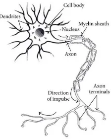
constructed NN, make a decision dependent to the neurons of the machine. Figure 2.3

outlines the similarities between a human neuron and a machine neuron [40]. A human

neuron consists of three major components: dendrites, cell body, and axon. Dendrites are

the inputs for the neuron’s cell body, receiving electrical impules and hormones from axons

(31)

15

impules it wants to send out through which axon, depending on the input from the

dentrities. In the human brain, there is on average 100 billion neurons connected to each

other though dendrites and axons. [41] Similarly, in a machine’s brain, the dendrites are

where the machine takes weighted inputs, and calculates the desired output, which is

processed through an activation function, and then either send out to next layer of NN, or

it is an output. The equation of a NN process is shown in Figure 2.3 [40], as Xo being the

input to the synapose of weight Wo, by which the input is multiplied. Following is the

summation of the inputs and the weights’ multiplications and an added bias, which

produces the final output from that neuron.

Figure 2.3: Neural Network Comparison between Human and Machine [40]

As it can be seen, MT and NNs has been around for a while; as shown in [8 – 11],

[37], [39], [42 – 48]. Table 2.4 contains few articles for major comparison; the articles were

chosen according to their effectiveness of delivering information and their reliability. As

can be seen from the table below, the majority of accurate literature review done

concerning DL and/or MT is written within the last decade, meaning that this topic of

research is still new. One major note concerning MT is that it needs a GPU (graphics

processing unit) to process extensive amounts of data at reasonable time, and in the future,

at real-time. The main difference between CPUs (central processing units) and GPUs is

that CPUs usually consist of few cores (usually about four), with big cache memory to

(32)

16

simultaneously execute instructions [49]. Furthermore, from inspecting Table 2.4, the

different types of NNs include (but are not limited to) CNN (convolution neural network),

KNN (K-nearest neighbor), ELM (extreme learning machine), and CUDA (computer

unified device architecture; acronym was dropped by Nvidia). Each of these NNs contain

their own advantages and disadvantages but are effectively overall the same since their

accuracy rate is comparable.

Table 2.4: Deep Learning Comparison

Articles YOLO/

OpenCV Uses GPU Neural Network Accuracy

A Comparative Study of Open Source Deep Learning

Framework (2018) [8]

NO YES YES (CNN,

TensorFlow DL)

Irrelevant

Automatic Vehicle Identification System using Machine Learning and Robot Operating System (ROS) (2017) [9]

YES (OpenCV)

NO YES (K-NN) 94.52%

Chinese Vehicle License Plate Recognition using Kernal-Based Extreme Learning Machine with Deep Convolutional Features (2017) [44]

NO YES YES (ELM

and CNN)

91.07%

Deep Learning System for Automatic License Plate

Detection and Recognition (2017) [39]

YES (YOLO)

NO YES (CNN) 94.8%

Evaluating the Power Efficiency of Deep Learning Inference on Embedded GPU Systems (2017) [45]

Yes (OpenCV

and YOLO)

YES YES (CUDA

with cuDNN)

Irrelevant

License Plate Recognition Application using Extreme Learning Machine (2014) [37]

(33)

17

2.3.3: Advantages of using Machine Training for Data Extraction

As can be seen from Table 2.3, IP has many disadvantages, even when a hybrid

(multiple IP techniques used together) model is created because of its complexity and

limitations. There are many everyday conditions that would cause noise in the images,

making the extraction of license plates difficult, and possibly inaccurate. While with a MT

model, a computer could be trained to accurately detect license plates in many different

environmental conditions. Furthermore, MT have been proven to be more accurate than IP,

as shown in Table 2.4. The process of IP would have to run on each individual image, while

a trained machine would process the images through its NN just once to create a successful

model that would quickly determine whether a certain object is present in a given image or

not.

2.4: Distance Detection

There are multiple different methods of distance detection between vehicles already

existing, with systems like ADAS. Current ADAS provide adaptive cruise control,

collision avoidance, pedestrian crash avoidance mitigation, incorporate traffic warnings,

connect to smartphones, alert driver to other cars or danger, lane departure warning system,

automatic lane centering, and show what is in blind spots; as mentioned in [50]. When

measuring distances between vehicles, accuracy becomes more critical as the vehicles’

speed increases. For example, if a vehicle is traveling at a constant speed of 100km/hr, in

perspective its traveling 27.7meters ever second. Computers for AV have to be constructed

to calculate and make decisions within one-third a second limit of real-time or less for

safety of the vehicle and surrounding environment.

2.4.1: Vehicle Detection

Vehicle detection is a very popular method for applying ADAS. As shown in [5],

[6], [9 – 12], [16], [21], [39] [47], vehicle detection was applied to attain distance between

(34)

18

used in [9]. Both IP and MT were used in [39], and [47], which had higher accuracy rates,

but longer processing time. Through vehicle detection, it would not provide an accurate

distance detection, since the size of different vehicle models are not the same.

2.4.2: License Plate Detection

License plate detection was more common, appearing in the following articles: [5

– 7], [21], [25 – 29], [33], [35 – 38], [42 – 43], [45]. As can be seen through articles [5 –

7], [21], [25 – 27], [33], [35 – 36], [43], IP techniques were used to attain the location of

the license plates. From noise in the images, it would be hard to extract the license plate in

every scenario. In articles [28 – 29], [37], [42], [45] MT was used to attain the location of

the license plate in the image, increasing the accuracy rates significantly.

2.4.3: Advantages of License Plate Detection for Distance Detection

The main advantage of detecting license plates in comparison to detecting vehicles

for calculating the distance between vehicles is that license plates are always a constant

size in North America; while vehicle size is always changing. Upon research, Table 2.5

outlines the average length, width and height of vehicles, from [51]. As can be observed

from Table 2.5, vehicles width and height could range from 1.446m to 1.837m for height

and 1.729m to 1.942m for width; it’s hard to determine the distance of an object that has a

variety of sizes. Furthermore, Table 2.5 does not include motorcycles and trucks which

have a much wider range compared to regular vehicles. The different variety of vehicles is

large, making it difficult to create an algorithm using vehicles to detect an accurate

distance. However, license plates are the same size within all of North America. Table 2.6

compares articles that detected vehicles and license plates, showing that both methods of

detections have similar accuracies. In Table 2.6, the articles with an asterisk concerning

the distance detected. Upon trying to find articles or journal papers concerning detecting

the distances between vehicles, it was concluded that this is not a popular topic of research.

In [5], [6], [21] it was researched to detect both the license plates and the vehicles in aiding

(35)

19

understandably obtained higher accuracy, but when applied simultaneously the processing

time increased as shown in [6]. Furthermore, on average from Table 2.6, the accuracy of

detecting license plates is 93.8%, while the accuracy of detecting full vehicles is 90.275%.

The averages of the detection rates of the vehicles and the license plates come to show that

license plates are easier to detect, even though they are small compared to the vehicle.

Upon future research on [5], and [6], it was discovered that both articles used image

processing techniques to detect the license plates and the distance using the license plates.

Also, articles [6], [16], and [21] used image processing techniques to detect the distances

of the vehicles. Hence, this thesis focus will be to detect license plates, which is a static

size, using an artificial neural network to contribute a new topic to the academia field.

Table 2.5: Vehicle Sizes [51]

Size Type Average Size (meters - LxWxH)

(36)

20

Table 2.6: Comparison Between Vehicle and License Plate Detection

Articles Vehicle

Detection Accuracy

License Plate Detection Accuracy

Vision-Based Vehicle Detection for a Driver Assistance System (2011) [6] **

81.6% Distance

94% Distance

A Rough Vehicle Distance Measurement Method Using Monocular Vision and License Plate (2015) [5] **

(0.8m)

Building an Automatic Vehicle License-Plate Recognition System (2005) [28]

97%

Deep Representation and Stereo Vision Based Vehicle Detection (2015) [10]

98%

Stereo Vision-Based Vehicle Detection (2000) [16] ** 90% (1.5m) Research of Vehicle Monocular Measurement System

Based on Computer Vision (2013) [21] **

96% Distance HSI Color Based Vehicle License Plate Detection

(2008) [33]

89%

License Plate Character Segmentation Based on the Gabor Transform and Vector Quantization (2003) [35]

98%

License Plate Detection using Gabor Filter Banks and Texture Analysis (2011) [36]

92.5%

On-Road Vehicle Detection Using Gabor Filters and Support Vector Machines (2002) [39]

95%

Appearance-Based Brake-Lights Recognition Using Deep Learning and Vehicle Detection (2016) [52]

89%

An Autonomous License Plate Detection Method (2009) [53]

96%

A Pattern-Based Directional Element Extraction Method for Vehicle License Plate Detection in Complex Background (2011) [54]

96.5%

Vehicle License Plate Detection in Images (2010) [55] 87.4%

Vision-Based Vehicle Detection and Inter-Vehicle Distance Estimation (2012) [56]

84.6%

A Real-Time Visual-Based Front-Mounted Vehicle Collision Warning System (2013) [57]

88%

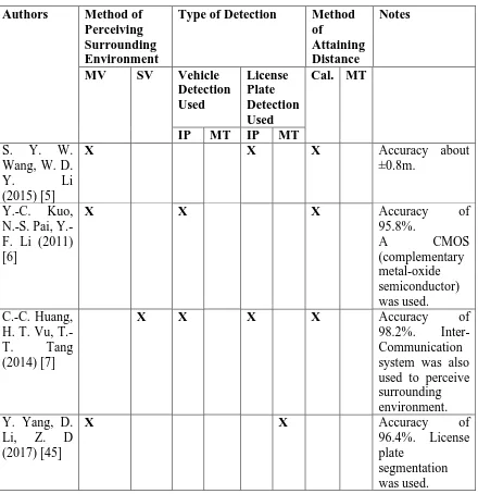
2.5: Related Work

A summary of related works covered in [5 – 7], [10], [16], [20 – 21], [29], [37],

[45] is outlined in Table 2.7. Key words used in Table 2.7 are as follows: MV is Monocular

(37)

21

calculated. As can be seen, a great deal different research has been done concerning

attaining vehicle distance using MV and MT for license plate detection. The focus of this

research is to detect the location of the license plate, and according to size of the license

plate, determine the distance of that vehicle.

Table 2.7a: Summary of Related Works

Authors Method of

Perceiving Surrounding Environment

Type of Detection Method

of

Attaining Distance

Notes

MV SV Vehicle

Detection Used License Plate Detection Used

Cal. MT

IP MT IP MT

S. Y. W. Wang, W. D.

Y. Li

(2015) [5]

X X X Accuracy about

±0.8m.

Y.-C. Kuo, N.-S. Pai, Y.-F. Li (2011) [6]

X X X Accuracy of

95.8%.

A CMOS

(complementary metal-oxide semiconductor) was used. C.-C. Huang,

H. T. Vu,

T.-T. Tang

(2014) [7]

X X X X Accuracy of

98.2%. Inter-Communication system was also used to perceive surrounding environment. Y. Yang, D.

Li, Z. D (2017) [45]

X X Accuracy of

96.4%. License plate

(38)

22

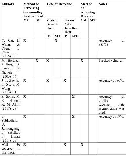
Table 2.7b: Summary of Related Works

Authors Method of

Perceiving Surrounding Environment

Type of Detection Method

of

Attaining Distance

Notes

MV SV Vehicle

Detection Used

License Plate Detection Used

Cal. MT

IP MT IP MT

Y. Cai, H.

Wang, X.

Chen, L.

Chen (2015) [10]

X X Accuracy of

98.7%.

M. Bertozzi, A. Broggi, A. Fascioli, S. Nichele (2003) [16]

X X X Tracked vehicles.

J.-T. Xue, S.-P. Xu, S.-M. Wang (2013) [21]

X X X Accuracy of 96%.

Z. Selmi, M. B. Halima, A. M. Alimi (2017) [29]

X X Accuracy of

91.3%.

License plate segmentation was used.

S.

Subhadhira, U.

Juithonglang, P. Sakulkoo P. Horata (2014) [37]

X X Accuracy of 89%.

Will be

covered in this thesis

(39)

23

From the table above, the combination of perceiving the surrounding environment

using MV, detecting license plates using MT, and attaining distance between vehicles using

calculations type of research has not been constructed yet. This thesis has aimed to attain

an accuracy of 90% or greater, which was surpassed. Furthermore, the majority of the

articles mentioned in Table 2.7 have only proven the theoretical approach concerning their

research topic, hence this thesis focuses on attaining an applicable approach of this ADAS

system. This thesis topic will be a good contribution to the academia society concerning

(40)

24

Chapter 3: Methodology and Description of Work

This chapter will cover the steps that were taken to complete this thesis, which is

shown in the block diagram in Figure 3.1. This thesis consists of three major steps:

1) obtaining a sufficient dataset that would aid in constructing a robust machine

trained model,

2) constructing a sufficient NN to train the machine with the dataset,

3) and putting together a localization and distance detection algorithms.

These steps are covered in depth in this chapter, along with additional steps required to

successfully replicate this project.

Figure 3.1: Thesis Flowchart

3.1: Obtaining a Dataset

In this thesis, a Nikon 1 J1 camera was used for MV. To achieve HD 1280x720

pixels for the images; the images were taken through the “movie” setting. It also contained

(41)

25

file data-type was a compressed 12-bit NEF (Nikon Electronic Format) RAW data. More

specs concerning the camera used in this thesis can be found in [58]. The first set of images

were taken in the University of Windsor’s Centre of Engineering and Innovation parking

lot with the mentioned camera and settings. Figure 3.2 shows the distance and location the

camera was placed for the images taken of the vehicles. The images were taken at distances

of 2m, 4m, 6m, 8m, 10m, 15m, 20m, 25m, and 30m. In addition, pictures were taken at the

same distances at angles 30° and 45° on left and right sides, where directly looking at the

vehicle is 0°, as outlined in Figure 3.2. With seven different vehicles, 267 images were

taken, according to the distances mentioned and labeled according to their location. For

example, Figure 3.3 is labelled as “car1_4_45L.JPG” which states that the image is of car

#1, at a distance of 4m and at an angle of 45° from the left side.

Figure 3.2: Layout of First Data-Set Image Taking

(42)

26

During training a NN, it was realized that the current data set was not sufficient

because the error rates barely went below a validation accuracy level of 60%, even after

more than thirty epochs; hence more images of license plates were obtained from online,

to be collaborated with the original data-set images. Certain amounts of images were taken

from the sites mentioned in Table 3.1. It was checked that there is no copyright violation

occurring when taking these images. A disadvantage of the online website images is that it

did not label the license plates’ distance from the camera which is needed for this thesis.A

great advantage about the following websites is that it contained license plate images from

every province and state from Canada, United States of America, and Mexico. This vast

variety of license plates aids in making the NN robust, and more applicable all-over North

America.

Table 3.1: Images taken from Online Websites

Website Number of Images

License Plate Mania [59] 647

The US 50 [60] 50

Olav’s License Plate Pictures [61] 217

Plates-Spotting [62] 255

License Plates of the World [63] 4054

Total 5223

3.2: Software Installation and Setup

To conduct the development of this research, GPUs and various Python packages

were used. Initial work was done on a Linux server, but later was transferred onto a

Windows computer. Table 3.2 covers the specs of the Linux server and the Windows OS

computer used. The next sub-sections cover the required major software used, installation,

(43)

27

Table 3.2: Specs of Used Computers

System Specs Linux Operating System Windows Operating System

Product Alienware Aurora R6 Asus Republic of Gamers GL753VD

Type Ubuntu 16.04.5 LTS Microsoft Windows 10 Home

Architecture X86_64 X64-based PC

Processor Intel® Core™ i7-7700K CPU

@ 4.20GHZ, 2400MHZ, 8 Cores

Intel® Core™ i7-7700HQ CPU @ 2.80GHZ, 2808MHZ, 4 Cores

Graphics Card

Nvidia GeForce GTX 1080 Ti Nvidia GeForce GTX 1050

RAM 16.0 GB 16.0 GB

Memory Size 2 TB HDD 1 TB HDD

3.2.1: OpenCV

OpenCV (Open Source Computer Vision Library) is an open source python

package containing libraries for CV and ML [64]. It was used in this thesis for CV, since

it had reliable algorithms for image processing. Minor errors and problems were resolved

through Google searches.

3.2.1.1: OpenCV on Linux – Ubuntu 16.04

Instructions from [65] were used to install OpenCV 3.4.4 onto Ubuntu 16.04.

Following the instructions to install OpenCV, the required OS libraries (which includes

cmake build) had to be installed initially, followed by python libraries. After installing

required packages, OpenCV and OpenCV_Contib’s githubs were installed, and built to be

used.

3.2.1.2: OpenCV on Windows 10

Similarly, [66] was used to install OpenCV 3 onto Windows 10. The required

applications included: Visual Studio 2015, CMake, and Anaconda. The installation process

for Windows is much lengthier and complicated. Anaconda installation is covered in the

(44)

28 3.2.2: Anaconda and Jupyter Notebook

Anaconda is a free platform for python programming language in an organized

environment. It supports virtual environments, which helps to keep different, conflicting

projects separated. Appendix A has all environments listed, along with the installation

command lines to install the libraries to the currently used environment. One of the

applications provided by Anaconda is Jupyter Notebook, which allows for the creation of

live code in virtual environments. The meaning of live code is that individual sections of

the code can be run without having to run the whole code.

Installation of Anaconda on Windows was already covered in the previous

subsection. For installing Anaconda on Linux, initially the latest Anaconda Linux Installer

was installed from Anaconda distribution website. The installation process mentioned in

[67] was followed with minor modifications to match the version installed and pathway

names on the used computer.

3.2.3: Tensorflow-GPU

Tensorflow is a platform for building a NN. Keras is an application that can be used

with tensorflow, making common neural network architecture (NNA) easier to code. Even

more, Tensorboard is created by tensorflow to help keep track of the NN as it trains.

Instructions to install tensorflow that is compatible with GPU is found at [68]. The process

of installing Tensorflow compatible with Nvidia GPU includes downloading CUDA and

cuDNN toolkits, which is covered in the instructions mentioned above.

3.2.4: GitHub

Microsoft created an online hosting service for code called GitHub. Using git

commands, the directory is easily uploaded onto the online repository. This thesis is saved

Vehicle Distance Detection Using Monocular Vision and Machine Learning

Scholarship at UWindsor

Scholarship at UWindsor

Vehicle Distance Detection Using Monocular Vision and Machine

Vehicle Distance Detection Using Monocular Vision and Machine

Learning

Learning

Vehicle Distance Detection Using Monocular

Vision and Machine Learning

By

Maryam Samir Naguib Girgis Hanna

A Thesis

Submitted to the Faculty of Graduate Studies

through the Department of Electrical and Computer Engineering

in Partial Fulfillment of the Requirements for

the Degree of Master of Applied Science

at the University of Windsor

Windsor, Ontario, Canada

2019

Vehicle Distance Detection Using Monocular

Vision and Machine Learning

By

Maryam Samir Naguib Girgis Hanna

Approved By:

S. Das

Department of Civil and Environmental Engineering

B. Balasingam

Department of Electrical and Computer Engineering

K. Tepe, Advisor

Department of Electrical and Computer Engineering

Declaration of Originality

Abstract

Dedication

I dedicate my thesis to my loving and supporting family;

Acknowledgements

Table of Contents

List of Figures

List of Tables

List of Equations

Abbreviations

Chapter 1: Introduction

1.1: Background

1.2: Motivation

1.3: Impacts of Autonomous Vehicles

1.4: Problem Statement

1.5: Thesis Contribution

1.6: Thesis Outline

Chapter 2: Literature Review

2.1: Background

2.2: Perceiving of the Surrounding Environment

2.3: Data Processing

2.4: Distance Detection

2.5: Related Work

Chapter 3: Methodology and Description of Work

3.1: Obtaining a Dataset

3.2: Software Installation and Setup