Development and Evaluation of Human Longitudinal
Time-Location-Activity Data
By Zeke Hill
Submitted to the Graduate Faculty of
North Carolina State University
In partial fulfillment of the
Requirements for the degree of
Master of Environmental Assessment
May 2014
Development and Evaluation of Human Longitudinal Time-Location-Activity Data
Abstract
Introduction
Fundamental to estimating exposure is the understanding of how an organism(s) of interest contacts various stressors. By definition, the basic tenets of exposure – duration, magnitude, frequency, and pattern – are dependent on these two components, that is, the variability (or lack of) in exposure results from the merging of contact rate and stressor level variability, all while considering the simultaneous sequencing of events for each component over short-term durations and/or extended periods (McCurdy, 2000). In estimating inhalation exposures, human time-location-activity patterns, detailed records of the places people visit (e.g., inside at home, outdoor amphitheater) and the activities performed (e.g., cooking, walking) within each, are a commonly used approach to accurately represent individual variability in stressor contact and their associated ventilation rate. For example, this type of approach has been used to estimate exposures and risk of adverse health responses by the United States (US) Environmental Protection Agency (EPA) in developing the National Ambient Air Quality Standards (NAAQS) for ozone (US EPA, 2007; US EPA, 2014), nitrogen dioxide (US EPA, 2008), sulfur dioxide (US EPA, 2009), carbon monoxide (US EPA, 2010).
In each of these assessments, The US EPA employed the Air Pollution Exposure (APEX) model, a
probabilistic population-based human exposure model that attempts to realistically capture both inter- and intra- personal variability in exposures via variability in how individuals go about their day (US EPA, 2012a,b). One key model input is EPA’s Consolidated Human Activity Database (CHAD), a collection of daily time-location-activity pattern data obtained from several national-scale and local surveys
(McCurdy et al., 2000; US EPA, 2002; Graham and McCurdy 2004). These data provide a daily time-series of personal locations visited and activities performed, and along with ambient pollutant concentrations and other anthropometric attributes, are used to estimate both short- and long-exposure concentrations along with each persons’ associated ventilation rates, often a critical factor in estimating important adverse health effects (US EPA, 2007; US EPA, 2009; US EPA, 2014).
There are limits to our understanding variability in stressor level and contact rate, perhaps more so for how contact is established and how activity patterns may vary over both short (daily) and longer (weekly, monthly) periods of time, particularly when considering an individual or groups of individuals. This is because much of the existing data are cross-sectional, that is to say, the original activity pattern survey in CHAD collected only a single diary day, representing a snapshot of an individual’s activity pattern. Advanced statistical methods have been developed to link seemingly unrelated diary days from multiple persons together to generate a longitudinal activity pattern profile for single simulated
research studies (e.g., having a limited study population group or sample size, few diary days collected, non-sequential days).
This is the underlying driver of the current investigation, to generate additional activity pattern data useful in inhalation exposure modeling and to improve our understanding of intra- and inter-variability in exposure by better characterizing trends in longitudinal time-location-activity data. The research performed here has been generally modeled after the recent longitudinal time-activity data study performed by Isaacs et al. (2012), though having significantly greater sample size. The project objectives include 1) develop basic though systematic data collection, processing, analysis, and associated quality assurance skills; 2) assign appropriate activity and location codes to each diary day to allow data to be incorporated within a widely used human time-location-activity pattern database; 3) determine the time spent within key exposure microenvironments visited and the time spent performing potentially
influential activities for the study participants; 4) perform advanced statistical evaluations of individual and group-level longitudinal activity patterns to better inform modeling efforts that estimate either peak exposure occurrences and/or cumulative intake doses ; 5) discuss assumptions made in data development and identifying important uncertainties that could affect conclusions.
Methodology
To generate new activity pattern data for CHAD and used by APEX and to investigate the longitudinal activity pattern data, personal time-location-activity diaries were generated by North Carolina State University (NCSU) Environmental Assessment (EA) students while completing coursework during the 2011 and 2013 fall semesters. The EA course in which the data was generated was instructed by Dr. Stephen Graham and Dr. Chris Hofelt whom have each specialized in environmental risk assessment field. Specific guidance on how to properly prepare personal diaries was presented during the course lectures and related examples were provided to better explain how to properly complete the “diary” work; I personally was involved as a student in the 2011 fall semester diary completion project and my personal results are included within the study. A template to be used by the students to document each activity and corresponding microenvironment was provided to be used. The instructors explained what types of activities needed to be documented and the specifics regarding required microenvironment information. Students were instructed to characterize their locations as to whether occurring indoors, outdoors, or inside a motor vehicle, though specificity of the type of microenvironment (inside
driving and the associated locations visited such as inside their residence, in a hotel, outside at a local park, or travelling in a car. The completion of the diary project and determining one’s exposure to benzene and ozone constituted approximately 20% of the student’s grade for the semester.
Out of the total number of students participating in the 2011 and 2013 semesters, 45 of them were selected here for additional analysis (yielding a total of 637 days).1 These diaries were selected based on
other similar longitudinal time activity data studies performed and what number would create a reliable representation of the population. Based on review of literature, the number of participants is relatively high for this study compared to similar studies. Diary data such as student gender, age and employment information surrounding the study group were selected for the analysis. Out of the total number of participants 53.3 % were male and 46.7 % were female. The age range of the total participant population spreads from 22 years to 54 years with a mean age of 31.8 years. The average age of the female participants is 29.1 and the average age of the male participants is 34.1. The maximum and minimum age for the male participants is 23 and 54 years; for the female participants, the maximum and minimum age is 22 and 38 years. Since the age range is so broad, four age categories were evaluated, ages 20 - 25 years (20% of the population), 26 – 30 years (40% of the population), 31 – 35 (17.8% of the population) years and 36 – 54 years (22.2 % of the population). The information is displayed within table 1 below.
Table 1: NCSU Activity Pattern Data Study Group Information.
Student ID M/FM Age Days Recorded
Occupation Type
Employed Fulltime Employment
13001 M 27 14 Labor Y N
13002 M 36 14 Prof Y Y
13003 F 31 15 Prof Y Y
13004 F 30 14 Prof Y Y
13005 M 24 14 Labor Y Y
13006 F 27 14 Admin Y Y
13007 F 25 14 Admin Y N
13008 M 48 14 Prof Y Y
13009 M 47 14 Prof Y Y
13010 M 54 14 NA NA NA
13011 M 33 14 Prof Y Y
13012 F 33 14 Prof Y Y
13013 F 23 14 NA NA NA
13014 F 34 14 Prof Y Y
13015 F 38 14 Prof Y N
13016 M 30 14 Prof Y Y
13017 M 23 14 Prof Y Y
13018 F 22 14 Serv Y N
13019 F 24 14 Prof Y N
13020 F 30 14 Prof Y Y
13021 F 24 14 Prof Y Y
13022 M 27 14 Prof Y Y
11001 M 30 14 Tech Y Y
11002 M 46 15 Tech Y Y
11003 M 36 14 Tech Y Y
11004 F 32 14 Prof Y Y
1 While 45 students generating 14-days would normally result in 630 total diary days, a few students apparently
11005 F 30 14 Tech Y Y
11006 F 26 14 Prof Y Y
11007 F 30 14 HSHL Y Y
11008 M 36 14 Prof Y Y
11010 M 30 15 Prof Y Y
11011 F 23 15 Prof Y N
11012 M 54 14 Prof Y Y
11013 M 35 14 Prof Y Y
11014 F 34 14 Tech Y Y
11015 M 35 15 Tech Y Y
11016 M 28 14 Prof Y Y
11017 F 37 14 Prof Y Y
11018 F 30 14 Admin Y N
11020 M 30 14 Serv Y Y
11023 F 29 14 Admin Y Y
11024 M 26 15 Admin Y Y
11025 M 29 15 Prof Y Y
11027 M 29 14 Admin Y Y
11028 M 26 14 NA NA NA
Each diary generated by the students during the two semesters that was selected for the analysis was evaluated for quality to determine if enough diary details had been obtained by the student to be useful in the longitudinal activity study. Overall, two diaries that had been completed during the 2011 and 2013 fall semesters and originally selected were eliminated from the study due to lack of specific details. The two diaries that were eliminated only included two to three microenvironments and only a few activities, therefore the data from the diary was determined to be unreliable and not specific enough. A diary with fewer than 30 events per day is generally considered to be “non-compliant(McCurdy and Graham, 2003; Graham and McCurdy, 2004) therefore diaries with fewer than 30 events per day recorded by the participant were not used within the study. The 45 remaining diaries that were
determined to provide effective data for study usage, were further adapted within an excel spreadsheet to include CHAD specific information such as activity codes and micro environmental codes (see
Appendix A, Figures A-1 and A-2). The diaries that were determined to be effective for our study contained at least 5 microenvironments and at least 15 activities within. Overall, for all diaries used there were approximately 30 CHAD activity codes assigned and approximately 20 CHAD
microenvironment codes assigned. Unique student identification codes were randomly assigned and times spent within each microenvironment were also outlined within the spreadsheets. Figure 1 below illustrates the format in which each useful diary was converted to for consistency purposes.
Figure 1: Excel Spread Sheet Template Used to Capture Relevant Data from Student Diary.
During the student diary information transfer to the excel spreadsheet from Figure 1, assumptions regarding the student’s activities and microenvironments had to be made. For example, a student’s diary may have indicated “bathroom” as an activity being performed; since “bathroom” does not have an activity code assigned in CHAD, the activity “personal care” was used. Another example of an
assumption made in assigning a student’s microenvironment is when one used “Outside residence”. It is unknown exactly what one’s outdoor residence may be like or if it’s next to a major highway,
construction site or park so the “General Outdoor” code was used. There were also situations when a student used multiple activities or microenvironments within their diaries. For example one may have indicated “Watching TV and Eating” as an activity; since there is a CHAD activity code for each of those one had to be selected. The activity that was ultimately selected during these situations was the activity that in my opinion required the most focus or exertion. In the example above, “Eating” was chosen as the activity by the student and “Watching TV” was disregarded. In addition, one may have indicated “In living room”, “In Bathrooom” or “In Kitchen” as their microenvironment; for simplification purposes, the CHAD location of “In-Residence” was selected to replace specific in residence locations. For purposes of data consistency and quality assurance, the corresponding student versus final activity and location descriptions were recorded for each diary as shown in column “loc_corr” and “act_corr” of Figure 1. For the purposes of developing activity pattern data for use in CHAD, all of the original descriptor data were retained for future purposes in the case different assumptions were needed or new and more
appropriate location or activity codes were developed.
General descriptive statistics were generated for locations visited using Microsoft Excel. All location data were mapped to three broad microenvironmental categories using the most current APEX CHAD microenvironemental mapping file (Appendix A Table A-2): Indoors, Outdoors,2 and In-Vehicle.
Estimation of day-to-day correlation statistics was done using SAS software (SAS Institute, Cary, NC).
Results
By assigning the NCSU project data appropriate CHAD codes, a total of 637 diary days are now usable by CHAD and for use in future exposure assessments that use such data. While this may seem of limited significance given that CHAD currently contains over 50,000 diary days, this is particularly important in that when simulating activities in a current or future exposure scenario, it is likely that the use of recently collected data more accurately represents the type of locations visited and level of activities performed. Note that some of the CHAD data were collected during the 1980’s, potentially occurring at a time not accounting for recent technological advances (e.g., personal video gaming activities) or changes in commuting or work patterns (e.g., tele-work opportunities) that would affect activity patterns. Further, the pool of longitudinal diaries has increased dramatically, giving potential to better reflect actual longitudinal profiles and increasing opportunities for further longitudinal data analysis research.
Out of the data collected during the 2011 and 2013 fall semesters, three main microenvironments where selected for a detailed analysis. The three main microenvironments include “Inside”, “Outside” and “In Vehicle”. To appropriately represent the time spent within each main microenvironment, the original diary CHAD codes had to be combined in many cases to fit into one of the three locations. Analysis of time spent within each microenvironment was performed and was further broken down into
certain categories such as day of the week, gender and age to evaluate if certain influences exist within the categories. Additionally, the analyses performed were also compared to other literature sources to determine if consistencies exist or if there are reasonable differences which is discussed in more detail within the next section.The mean or average time per day was used and was based on all people across the category of interest. There are multiple influences in the data that can be observed. For means of clarity, each microenvironment category is described that show signs of influencing factors.
The average time spend outdoors was greater on the weekend days versus the weekdays. This is observable from analyzing the data from each single day and by analyzing the data per weekday or weekend basis. As displayed in table 3e, the time spent outdoors on Saturday more than doubled the time spent outdoors during the weekdays. Time spent outdoors is also influenced by gender; the male gender spent considerably more time outdoors on both weekends and weekdays compared to the female gender. Lastly, the age category also influenced time spend outdoors with the age ranges of 26 – 30 (40 % of population) and 36 – 54 (22.2 % of population) spending a considerable amount of time outdoors compared to those in the age ranges of 20 – 25 (20 % of population) and 31 – 35 (17.8 % of population).. A broader age category of > 30 (40% of the population) or </= 30 (60% of the population) was also evaluated to see if the age influence still exists and the data revealed that the older age group generally spends more time outdoors.
Much like time spent outdoors, time spent indoors seems to be influenced by the same categories and by the fact that time spent indoors is negatively correlated with the time spent outdoors; therefore, we can somewhat predict the indoor time spent by knowing the outdoor time spent. More time is spent indoors on the weekdays versus the weekends and females spend more time indoors compared to males on both weekends and weekdays. The age categories explained in the outdoors
microenvironment predict what is presented in the indoor microenvironment, with the age groups of 22 – 25 and 31 – 35 spending the most time indoors compared to other two age groups. Overall, the time spent indoors occupies the vast majority one one’s time in this particular study.
Time in a vehicle is also influenced by the categories as well and there is a recognizable consistency within the data. Based on the weekday and weekend averages, more time is spent in a vehicle during the weekdays versus the weekends and males spend slightly more time within the microenvironment. However, the time spent within a vehicle is not consistent when observing each day of the week
individually; for example, slightly more time is spent within a vehicle on Saturday compared to Monday, Tuesday and Wednesday. Age groups did have an impact on time spent within a vehicle as well; age groups 26 – 30 and 36 – 54 spend more time within a vehicle compared to the 22 – 25 and 31 – 35 age groups. For details of the exact times spent within each microenvironment by each category see the tables 2 and 3a-3h.
Table 2: Time Expenditure Information
Location Category Minutes/Day Mean Minute/Day Minimum
Minute/Day Maximum
Inside Weekday 1216 30 1440
Weekend 1133 0 1440
Weekend 202 0 1365
Vehicle Weekday 112 0 690
Weekend 100 0 705
Table 3a – 3h: Expenditure by Influential Variables
Table 3a: Time Outdoors – Males
Category Number of Days & Males
Minutes/Day Mean Minute/Day Minimum Minute/Day Maximum
Weekend 182 & 24 228 0 1365
Weekday 455 & 24 131 0 1330
Table 3b: Time Outdoor – Female
Category Number of Days & Females Minutes/Day Mean Minute/Day Minimum Minute/Day Maximum
Weekend 182 & 21 171 160 1220
Weekday 455 & 21 82 0 532
Table 3c: Time Indoor – Males
Category Number of Days & Males Minutes/Day Mean Minute/Day Minimum Minute/Day Maximum
Weekend 182 & 24 1103 0 1440
Weekday 455 & 24 1186 30 1440
Table 3d: Time Indoor – Female
Category Number of Days & Females Minutes/Day Mean Minute/Day Minimum Minute/Day Maximum
Weekend 182 & 21 1168 160 1440
Weekday 455 & 21 1251 720 1440
Table 3e: Time in Vehicle – Male
Category Number of Days & Males Minutes/Day Mean Minute/Day Minimum Minute/Day Maximum
Weekend 182 & 24 101 0 480
Weekday 455 & 24 120 0 400
Table 3f: Time in Vehicle – Female
Category Number of Days & Females Minutes/Day Mean Minute/Day Minimum Minute/Day Maximum
Weekend 182 & 21 98 0 705
Weekday 455 & 21 104 0 690
Table 3g: Day of Week Breakdown
Category Number of Days Inside - Minutes/Day Mean Inside – Minutes/Day Min : Max
Outside - Minutes/Day Mean
Outside – Minutes/Day Min : Max
Vehicle - Minutes/Day Mean
Monday 92 1234 606 : 1440 100 0 : 640 102 0 : 400 Tuesday 91 1227 588 : 1440 108 0 : 647 104 0 : 333 Wednesday 92 1224 435 : 1440 107 0 : 685 106 0 : 450 Thursday 90 1217 30 : 1410 111 0 : 1330 112 0 : 690 Friday 91 1179 510 : 1378 115 0 : 635 138 10 : 410 Saturday 91 1077 0 : 1440 249 0 : 1365 109 0 : 705 Sunday 90 1188 0 : 1440 155 0 : 1215 91 0 : 404
Table 3h: Age Group
Data Comparison / Discussion of Results
The results obtained from the study were compared to other longitudinal time-activity data sets that have been compiled in order to evaluate the consistencies and differences in the information. The primary information compared was time spent by the students within the microenvironments in the tables above to other datasets in which the same microenvironment data time spent was evaluated.
Comparison 1:
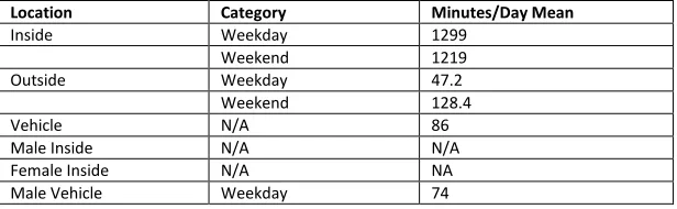
One study titled “Statistical properties of longitudinal time-activity data for use in human exposure modeling” (alsomentioned above and used as a model for the current project) performed by Isaacs et al explored the daily activity patterns of eight working adults within the Raleigh, North Carolina region between the ages of 35 - 66. The total number of data collection days was much greater by the eight working adults compared to the data collected by the students (~ 52 days of data collection data
averaged per adult versus ~ 14 days of data collection averaged per student) and the data collection was seasonal which is an important consideration considering temperature difference; however, the number of events recorded per day was consistent between the two studies.
Comparison of Time Expenditure Information
Location Category Minutes/Day Mean
Inside Weekday 1299
Weekend 1219
Outside Weekday 47.2
Weekend 128.4
Vehicle N/A 86
Male Inside N/A N/A
Female Inside N/A NA Male Vehicle Weekday 74
Age Category (Years) Number in Category Inside - Minutes/Day Mean Inside – Minutes/Day Min : Max
Outside - Minutes/Day Mean
Outside – Minutes/Day Min : Max
Vehicle - Minutes/Day Mean
Vehicle – Minutes/Day Min : Max
Weekend 86 Female Vehicle Weekday 27 Weekend 125
Comparison 2:
Another study reviewed titled “Using human activity data in exposure models: Analysis of discriminating factors” by McCurdy et al, evaluated the differences between a cross sectional sample and a longitudinal individual to evaluate the differences in time spent within certain microenvironments that can be attributed to certain discriminating factors. For purposes of comparison of data obtained from the students, the information was in the table below illustrates data pulled from the research that compares the two examples.
Comparison of Time Expenditure Information
Location Minutes/Day Mean Cross Sectional Sample
Inside 1224 Outside 176 Vehicle 107
Longitudinal Sample
Inside 1228 Outside 125 Vehicle 106
Longitudinal Statistical Review
To simulate long-term exposures (e.g., weekly, monthly or annual), EPA has developed a longitudinal diary-construction approach, that is, a method to link together diary data in CHAD that are cross sectional in nature (US EPA, 2012). This population diversity- and autocorrelation- (D & A) based
method attempts to reproduce both individual and population-level variability in time expenditure, both factors important in estimating exposures.
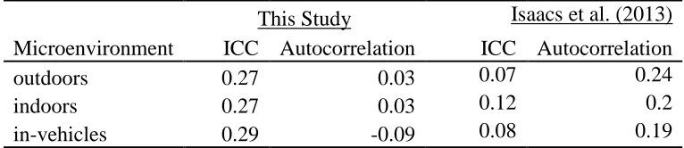
The longitudinal diary measurement data generated for this project were used to estimate the two variables needed when performing exposure modeling that use this D & A method. As was done in Isaacs et al. (2013), an intraclass correlation coefficient (ICC) was estimated and used to represent the diversity (D) statistic for three broadly defined microenvironments (time spent indoors, outdoors, and inside motor vehicles) using the fraction of inter-personal (or between person, 𝜎𝑏2) variability relative to the intra-personal (within person variability, 𝜎𝑤2) variability. Both of the variability components were generated with SAS using PROC ANOVA, whereas the ICC was calculated as follows:
𝐼𝐶𝐶 = 𝜎𝑏2/(𝜎
𝑏2+ 𝜎𝑤2)
A mean population day-to-day correlation statistic was calculated, that is a lag 1 (one-day)
autocorrelations were calculated using the SAS PROC CORR procedure. Estimates of the ICC and A using the longitudinal data are provided below in Table 4.
Table 4. Intraclass correlation coefficient (ICC) and autocorrelation (A)
statistic estimated using the longitudinal diary data.
Microenvironment
This Study
Isaacs et al. (2013)
ICC Autocorrelation
ICC Autocorrelation
outdoors
0.27
0.03
0.07
0.24
indoors
0.27
0.03
0.12
0.2
in-vehicles
0.29
-0.09
0.08
0.19
Results for the ICC statistic generated here are generally higher than the range of values calculated by Isaacs et al. (2013) for their adult study group, while autocorrelation statistics estimated in this study were generally lower when comparing similar microenvironments. Values for the ICC indicate a large degree of within-person variability in time expenditure, possibly driven by the underlying nature of many of the diary persons. In reviewing some of the locations listed, there appeared to be a number of study subjects that periodically spent work time outdoors as well as time spent in hotels, probably driven by their specific occupational duties (e.g., environmental field sampling events). This behavior could also explain the low autocorrelation statistic, that is, these study subjects do not appear to have significant day-to-day repetition in the locations where they spend time.
Conclusions
The data in this paper represents the longitudinal time activity patterns and a statistical analysis from graduate students participating in EA 503. There were 45 student diaries that were used in the analysis which comprised a total of 637 days of data. The objectives of the study were to 1) develop basic though systematic data collection, processing, analysis, and associated quality assurance skills; 2) assign appropriate activity and location codes to each diary day to allow data to be incorporated within a widely used human time-location-activity pattern database; 3) determine the time spent within key exposure microenvironments visited and the time spent performing potentially influential activities for the study participants; 4) perform advanced statistical evaluations of individual and group-level longitudinal activity patterns to better inform modeling efforts that estimate either peak exposure occurrences and/or cumulative intake doses ; 5) discuss assumptions made in data development and identifying important uncertainties that could affect conclusions.
The data used within the study was obtained from the graduate students using data collection methods taught within EA 503 which included the completion of detailed daily activity pattern diaries. Each diary was assessed for quality purposes and the 45 diaries selected displayed an adequate amount of
it’s unlikely that the assumptions made affected the quality of the data since the assumptions made were much more specific (i.e. changed “bathroom” to “inside residence”).
The time spent within each location showed that slight influencing variables exist such as time spent outdoors is higher for males on both weekends and weekdays. In addition, time spend outdoors for each individual group (age, gender) is higher on the weekend days. These findings are consistent with similar activity pattern studies that have been performed. The time spent within each
micro-environment by age groups shows a minor influence; based on the diary participant’s age range (22 years to 54 years) the ages of 22-25 years and 31-35 years are closer in correlation and the ages of 26-30 and 36-54 are closer in correlation.
The intraclass correlation coefficient (ICC) and autocorrelation (A) statistic findings were somewhat different than what we expected going into the project while comparing findings to a recently
conducted longitudinal activity analysis. Our study indicated an ICC range of .27 through .29 and an A range of .03 through -.09. These values indicate that the group of individuals have a high degree of within person variability and do not appear to have common day to day repetition of activities. These findings can be attributed to the specifics of the group studied. In reviewing the data, it’s evident that each student’s diary attributes are unique; the main correlation is the situation that each student was enrolled within EA 503 which is a distance learning course, so even that particular activity (Adult Education or Homework) would not necessary produce consistency to activity patterns. The group of students evaluated within the study held different types of occupations, lived in various locations and exhibited a wide age range which would have an effect on activities and locations visited. The other longitudinal activity pattern statistical analysis performed by Isaacs et al included individuals with more similar patterns such as, they worked in the same field, held similar work hours, and lived/worked in the same area which apparently leads to less of an effect on the differences in activities performed and locations visited.
Overall, the results of the study help prove that we can predict high within person variability even with longitudinal time activity studies which can be used to help improve our ability of appropriately
References
Glen, G.; L. Smith; K. Isaacs; T. McCurdy and J. Langstaff. 2008. "A New Method of Longitudinal Diary Assembly for Human Exposure Modeling." Journal of Exposure Science and Environmental Epidemiology, 18:299-311.
Graham, S. E. and T. McCurdy. 2004. "Developing Meaningful Cohorts for Human Exposure Models."
Journal of Exposure Analysis and Environmental Epidemiology, 14:23-43.
Knowledge Networks. (2009). Field Report: National-Scale Activity Survey (NSAS). Conducted for Research Triangle Institute. Submitted to Carol Mansfield November 13, 2009.
Isaacs, K. K., McCurdy, T., Glen, G., Nysewander, M., Errickson, A., Forbes, S., Graham, S., McCurdy, L., Smith, L., Tulve, N., and Vallero, D. (2012). Statistical properties of longitudinal time-activity data for use in human exposure modeling. Journal of Exposure Science and Environmental
Epidemiology. 23(3): 328-336.
McCurdy, T. 2000. "Conceptual Basis for Multi-route Intake Dose Modeling Using an Energy Expenditure Approach.” Journal of Exposure Analysis and Environmental Epidemiology, 10:1-12.
McCurdy, T.; G. Glen; L. Smith and Y. Lakkadi. 2000. "The National Exposure Research Laboratory's Consolidated Human Activity Database." Journal of Exposure Analysis and Environmental Epidemiology, 10:566-578.
McCurdy, T., Graham, S. E. (2003). Using human activity data in exposure models: analysis of discriminating factors. J Expos Anal Environ Epidemiol. 13(4): 294-317.
US EPA. 2002. Consolidated Human Activities Database (CHAD) Users Guide. Database and documentation available at: <http://www.epa.gov/chadnet1/>.
US EPA. 2007. Ozone Population Exposure Analysis for Selected Urban Areas. Research Triangle Park, NC: EPA Office of Air Quality Planning and Standards. Available at:
<http://www.epa.gov/ttn/naaqs/standards/ozone/s_o3_cr_td.html>.
US EPA. 2008. Risk and Exposure Assessment to Support the Review of the NO2 Primary National Ambient
Air Quality Standard. Washington, DC: EPA Office of Air and Radiation. (EPA document number EPA-452/R-08-008a0, November). Available at:
<http://www.epa.gov/ttn/naaqs/standards/nox/data/20081121_NO2_REA_final.pdf>.
US EPA. 2009. Risk and Exposure Assessment to Support the Review of the SO2 Primary National Ambient
Air Quality Standard. (EPA document number EPA-452/R-09-007, August). Available at: <http://www.epa.gov/ttn/naaqs/standards/so2/data/200908SO2REAFinalReport.pdf>.
US EPA. 2010. Quantitative Risk and Exposure Assessment for Carbon Monoxide – Amended. Research Triangle Park, NC: EPA Office of Air Quality Planning and Standards. (EPA document number EPA-452/R-10-009, July). Available at: <http://www.epa.gov/ttn/naaqs/standards/co/data/CO-REA-Amended-July2010.pdf>.
US EPA. 2012a. Total Risk Integrated Methodology (TRIM) - Air Pollutants Exposure Model
NC: EPA Office of Air Quality Planning and Standards. (EPA document number EPA-452/B-12-001a). Available at: <http://www.epa.gov/ttn/fera/human_apex.html>.
US EPA. 2012b. Total Risk Integrated Methodology (TRIM) - Air Pollutants Exposure Model
Documentation (TRIM.Expo / APEX, Version 4.4) Volume II: Technical Support Document. Research Triangle Park, NC: EPA Office of Air Quality Planning and Standards. (EPA document number EPA-452/B-12-001b). Available at: <http://www.epa.gov/ttn/fera/human_apex.html>.
US EPA. 2014. Health Risk and Exposure Assessment for Ozone. Second External Review Draft. Research Triangle Park, NC: EPA Office of Air Quality Planning and Standards. (EPA document number EPA EPA-452/P-14-004a). Available at:
<http://www.epa.gov/ttn/naaqs/standards/ozone/data/20140131healthrea.pdf >.
APPENDIX A