ABSTRACT
WENG, TENGYING. The Dynamics of the US Broiler Industry. (Under the direction of Tomislav Vukina and Xiaoyong Zheng.)
This essay studies the effect of higher concentration of US broiler industry on social welfare
and effect of productivity and demand-specific factors on plants’ probability of survival,
ownership change and firms’ probability of expansion. My results show that producer surplus
increased when concentration increased, and decreased when centration decreased; consumer
welfare increased as a result of lower price; and social welfare changed in the same direction
as producer surplus. My results also show that higher demand-specific factors will increase
the probability of survival, probability of ownership change and probability of expansion.
© Copyright 2012 by Tengying Weng
The Dynamic of the US Broiler Industry
by
Tengying Weng
A dissertation submitted to the Graduate Faculty of North Carolina State University
in partial fulfillment of the requirements for the Degree of
Doctor of Philosophy
Economics
Raleigh, North Carolina
2013
APPROVED BY:
_______________________________ ______________________________
Tomislav Vukina Xiaoyong Zheng Committee Co-Chair Committee Co-Chair
________________________________ ________________________________
BIOGRAPHY
Tengying Weng is the only daughter of Guoqiang Weng and Yunhua Sheng. She was born
on July 21, 1985, in China. From 2004 to 2008, she attended Zhejiang University, one the
most prestigious universities in China. Ms. Weng received a B.S. degree in Environmental
and Resource Science in 2008.
After receiving her bachelor’s degree, Ms. Weng enrolled in the Economics graduate
program at North Carolina State University at the master’s level. She changed from the
terminal master’s program to the Ph.D. program in December 2007. She finally earned a
Ph.D. degree in Economics in May 2013.
ACKNOWLEDGMENTS
I am grateful to Dr. Tomislav Vukina and Dr. Xiaoyong Zheng, my supervisors, for
their many suggestions and constant support during this research. Without their support, I
would not have accomplished this task. I would like to express my appreciation to Dr.
Michael Wohlgenant for his advice and great help on my chapter 3. I would like to thank Dr.
Robert Hammond who suggested several ideas on how to tackle many questions in this
dissertation.
I gratefully acknowledge the USDA-ERS for providing the data used in chapter 3 and
chapter 4. I would also like to thank Bert Grider (UNC) for his help on using the Census data
used in chapter 3 and chapter 4.
Very specific thanks go to my family, especially my dad and my mom, for their
patience and support. Without them, this research would never have come to existence. I
thank my brother, Tengfei, for offering encouragement throughout this research.
Finally, I wish to thank the following: Bidong Liu (for support), Tingting Liu, Luyuan
Niu, Xiaomei Chen, Xingyi Su (for friendship) and friends from Zhejiang University. I also
TABLE OF CONTENTS
LIST OF TABLES ... vi
LIST OF FIGURES ... vii
CHAPTER 1: INTRODUCTION ... 1
CHAPTER 2: THE U.S. BROILER INDUSTRY ... 4
2.1 A Brief History ... 4
2.2 More Recent Developments ... 5
2.3 Industry Structure and Dynamics ... 7
2.4 Today’s Industry ... 9
CHAPTER 3: WELFARE EFFECTS OF THE HORTIZONTAL CONSOLIDATION IN THE BROILER INDUSTRY ... 20
3.1 Introduction ... 20
3.2 Literature review ... 21
3.2.1 Theoretical Literature... 21
3.2.2 Empirical Literature ... 25
3.3 Empirical Methodology... 27
3.3.1 Producer Surplus ... 27
3.3.1.1 Cost Function Estimation ... 27
3.3.1.2 Producer Surplus ... 30
3.3.2.1 Estimating Demand for Chickens ... 32
3.3.2.2 Change in Consumer Surplus ... 34
3.3.3 Compensating Variation ... 38
3.4 Data ... 39
3.4.1 Census data ... 39
3.4.2 USDA Data ... 42
3.5 Results ... 44
3.5.1 Producer Surplus ... 44
3.5.2 Demand Estimation ... 47
3.5.3 Consumer Surplus and Compensating Variation ... 49
3.5.4 Changes in Social Welfare ... 51
CHAPTER 4: THE EFFECTS OF PRODUCTIVITY AND DEMAND-SPECIFIC
FACTORS ON PLANTS’ SURVIVAL AND OWNERSHIP CHANGE ... 68
4.1. Introduction ... 68
4.2. Theoretical Framework ... 73
4.3. Data and Measurement Issues ... 80
4.3.1. Measuring Productivity ... 82
4.3.2. Measuring Demand-Specific Factors ... 86
4.4. Estimation Models... 87
4.5. Results ... 89
4.5.1 Plant-Level Analysis ... 90
4.5.2 Firm-Level Analysis ... 92
4.6. Conclusions ... 95
CHAPTER 5: CONCLUSION ... 105
REFERENCES ... 108
APPENDIX ... 113
LIST OF TABLES
Table 1: Growth in Broiler Production (%), 1987-2007 ... 10
Table 2: Major Mergers and Acquisitions among Top 25 firms, 1997- 2009 ... 11
Table 3: National Rankings of Broiler Companies, 1997-2009 ... 12
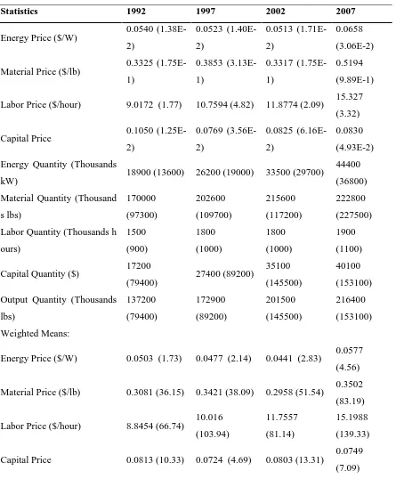
Table 3.1: Summary Statistics for Cost Function Estimations, 1992-2007 ... 54
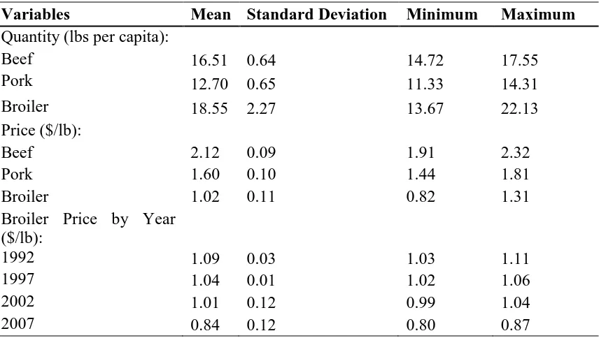
Table 3.2: Summary Statistics of Retail Prices and Consumption Quantities for Meats, 1989-2009... 55
Table 3.3: Generalized Leontief Cost Function and Input Demand System Estimation Results ... 56
Table 3.4: Input Demand Elasticity ... 58
Table 3.5: Producer Surplus, 1992-2007 ... 60
Table 3.6: LA/AIDS Demand System Estimation Results ... 61
Table 3.7: Uncompensated Price and Income Elasticities ... 62
Table 3.8: Compensated Price Elasticities ... 63
Table 3.9: Extreme Prices, 1992-2007 ... 64
Table 3.10: Change in Consumer Surplus per Capita ($) ... 64
Table 3.11: Compensating Variation ($) ... 65
Table 3.12: Social Welfare Changes per Capita ($) ... 65
Table 4.1: Summary Statistics for Variables Used to Calculate Physical Productivity and Demand Specific Factors (1987-2002) ... 96
Table 4.2: Summary Statistics for Plant-Level Physical Productivity and Demand Specific Factors (1987-2002) ... 97
Table 4.3: Plant-level Demand Estimation Results Using 2SLS ... 98
Table 4.4: Probability of Plant Exit ... 99
Table 4.5: Probability of Ownership Change ... 100
Table 4.6: Estimation Results for Multinomial Model ... 101
Table 4.7: Marginal Effects of One-Standard-Deviation Increase ... 102
Table 4.8: Firm-level Physical Productivity and Demand-specific Factors (1987-2002) .... 102
Table 4.9: Firm-level Demand Estimation Results with 2SLS ... 103
LIST OF FIGURES
Figure 1: US Broiler Production (million lbs), 1987-2010 ... 13
Figure 2: Meat Consumption per Capita (lbs), 1987-2010 ... 14
Figure 3: Meat Real Retail Prices (dollars/lb), 1989-2009 ... 15
Figure 4: Retail Prices of Beef and Pork Relative to Broilers, 1989-2009 ... 16
Figure 5: Expenditure Shares of Meat on Food Expenditure (%), 1987-2009 ... 17
Figure 6: US Broiler Exports (million lbs), 1987-2010 ... 18
Figure 7: US Broiler Export Ratio in Values (%), 1987-2010 ... 19
Figure 3.1: Demand Curve for Chicken when ... 66
CHAPTER 1: INTRODUCTION
The US broiler industry is generally considered to be the role model of industrialized
agriculture in the United States. There are three characteristics which make the US broiler
industry special and interesting. First, the US broiler industry is almost entirely vertically
integrated, from breeding flocks and hatcheries to feed mills, transportation divisions and
processing plants. The only stage which is not integrated with processors is farmers
(commonly called growers). Today, more than 90% of broiler chickens are raised under
contract. Because of the significant economies of scale and a large proportion of the value
added in processing, processors became the natural leaders of the industry. Second, the US
broiler industry has become more and more concentrated during the last couple of decades.
The Herfindahl index (HHI) of poultry processing industry increased from 735 to 1224 from
1992 to 2007.1 The industry's Top-4 concentration ratio increased from 44.24% in 1992 to
58.52% in 2007, and its Top-8 concentration ratio increased from 60.30% to 72.14%.2
Finally, the total production of the US broiler industry increased dramatically from 1992 to
2007. In fact, chicken consumption surpassed beef consumption in 1993 and became the
number-one meat item consumed in the United States. In Chapter 2, I will explore these
aspects of the broiler industry’s history.
As mentioned above, the US broiler industry became more and more concentrated
during the study period. The higher concentration in the US broiler industry could decrease
the social welfare (because of higher market power) or increase social welfare (because of
1
In the calculation of HHI, I picked the top 50 firms and left the rest of firms in the “other” category with Census data of Manufacture.
2 Top-4 and Top-8 are the top 4 firms’ market shares and top 8 firms’ market shares in the value of shipments
higher efficiency). So the objective of Chapter 3 is to determine which one of the two effects
dominates. In other words, are the cost reductions (synergies) through consolidation enough
to offset the allocation inefficiency resulting from greater market power? The results of this
analysis show that the overall social welfare increased during the HHI’s increasing period
(1992-2002) while decreasing during the HHI’s decreasing period (2002 to 2007). These
results show that society benefited from higher concentration in the poultry industry, while it
worse off from lower concentration in the poultry industry.
The possible sources of increasing concentration of the US broiler industry are
mergers and acquisitions, exits, and expansions. So one of the major objectives of Chapter 4
is to determine which plants were more likely to exit (the effects of productivity and
demand-specific factor). Generally speaking, people believe that plants with higher productivity are
less likely to exit. But most previous studies used revenue-based productivity as a measure of
physical productivity because of the availability of data. This method could overstate the
effect of physical productivity because revenue-based productivity combines with physical
productivity and specific factors. Chapter 4 explains the definition of
demand-specific factors and why using revenue productivity could overstate the effect of physical
productivity. By separately estimating the effect of physical productivity and
demand-specific factors on plants’ survival, I show that higher demand-demand-specific factors decrease the
probability of exit. The effect of physical productivity on the probability of exit is generally
insignificant. In addition to studying the effect of physical productivity and demand-specific
factors on the probability of a plant’s exit, I also study the effect of these factors on the
Most previous studies treat plants’ ownership change as plants exit; however, I
decided to separate ownership changes from exits, mainly because I believe plants that
change ownership are fundamentally different from plants that completely exit from the
industry. Plants that change ownership have to be good enough to attract other firms to buy
them. The results of this study show that higher demand-specific factors increase the
probability of an ownership change, while the effect of physical productivity on the
probability of an ownership change is generally insignificant. Finally, given the fact that the
poultry industry’s volume of production has almost doubled during the studied period, I also
analyze the firm-level expansion in Chapter 4. The results show that firms with higher
demand-specific factors have a higher probability to expand their businesses.
Overall, our results show that the effect of physical productivity is not significant and
that previous studies that used revenue productivity overstated the effect of physical
productivity. Instead, demand-specific factors have significant effects on the probability of a
plant’s exit, ownership change, and on firms’ expanding. Also, it is necessary to separate
plants that change ownership change from plants that exit, because the results of this study
show that demand-specific factors have opposite effects on the probability of exit and
ownership change. By treating plants that change ownership as plants that exit the broiler
industry altogether, previous studies could have possibly underestimated the effects of
CHAPTER 2: THE U.S. BROILER INDUSTRY
The broiler industry is generally considered to be the role model of industrialized
agriculture in the United States. In the last century, the U.S. broiler industry has evolved
from disorganized and locally-oriented business into a highly efficient, vertically integrated
and horizontally concentrated industry that provides products nationwide and around the
globe. This chapter presents a brief description of the U.S. broiler industry.
2.1 A Brief History
About 100 years ago, the United States chicken industry consisted of millions of small
households raising flocks of dual-purpose chickens (eggs and meat) in their backyards. Mrs.
Wilmer Steele of Sussex County, Delaware, is believed to be the pioneer US broiler (a
chicken raised specifically for its meat) industry. In 1923, she raised a flock of 500 broilers.
Her business turned out to be successful; consequently, in 1927 she was able to build a
broiler house with a capacity of 25,000 broilers. By 1952, accompanied by the improvement
in technology (e.g. on-line evisceration and discovery of the importance of nutrition and
photoperiod (cycle of sunlight and darkness) on production), specially bred meat chickens
(broilers) surpassed the farm chickens and became the number one source of chicken meat in
the United States.
The further technological developments in all stages of the industry led to
overproduction and hence lower prices. The substantial losses in 1959 and 1961, due to
excess production and the lack of coordination between feed mills, hatcheries, farms and
processors, caused a large exit of hatcheries and feed companies from the broiler industry
the industry. Because of the significant economies of scale and a large proportion of the
value added in processing, processors became the natural leaders of the industry. By the
1970s, the broiler chicken industry had evolved into the fully integrated industry seen today
where more than 90% of the broilers production came from integrated operations.
2.2 More Recent Developments
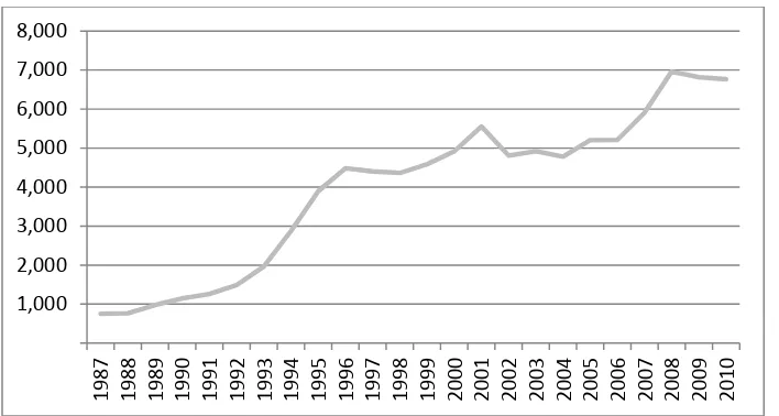
From 1987 to 2007, the production of broilers in the USA grew rapidly (see Figure 1).
Compared to 15,413 million pounds in 1987, the total broiler production was 35,772 million
pounds in 2007. Three main factors contributed to this growth: growth in population, growth
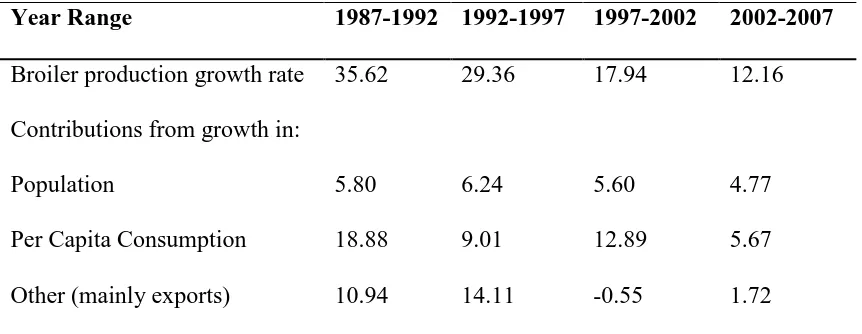
in per capita consumption, and exports. Table 1 shows the contributions of those factors in
5-year intervals between 1987 and 2007. As seen from the data, the most significant
contribution came from the growth in per capita consumption which was as high as almost
19% in the 1987-1992 period (see also Figure 2 which depicts the trend in the per capita
broiler consumption for the 1989-2009 period). Chicken consumption surpassed beef
consumption in 1993 and became the number one meat item consumed in the United States.
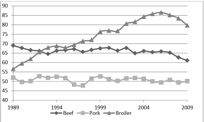
The growth in the volume of production was accompanied by the decrease in price. As
illustrated in Figure 3, broiler retail price dropped from $1.16/lb in 1987 to $0.89/lb in 2007,
whereas for its substitutes, beef and pork, prices remained relatively stable.3
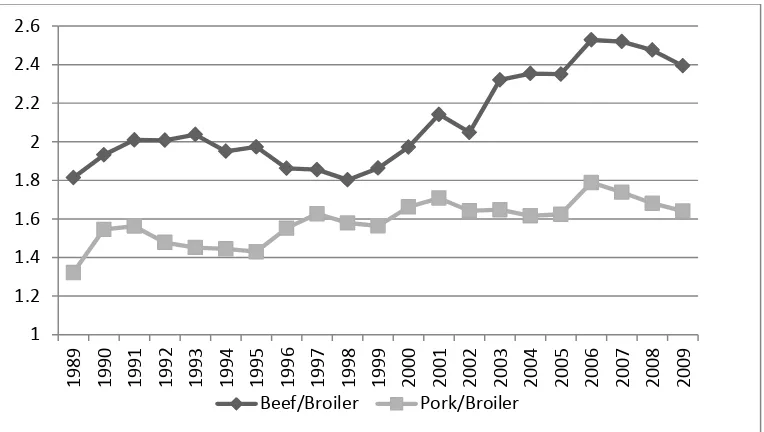
The growth in the broiler per capita consumption may be explained by a couple of
factors. The first is the reduction in the relative price of chicken meat compared to its
substitutes, beef and pork. As seen from Figure 4, the ratio of beef price to broiler price
3 Meat prices were calculated by averaging the quarterly prices deflated by meat consumer price index from
increased from 1.8 in 1989 to 2.5 in 2007, and the ratio of pork price to broiler price
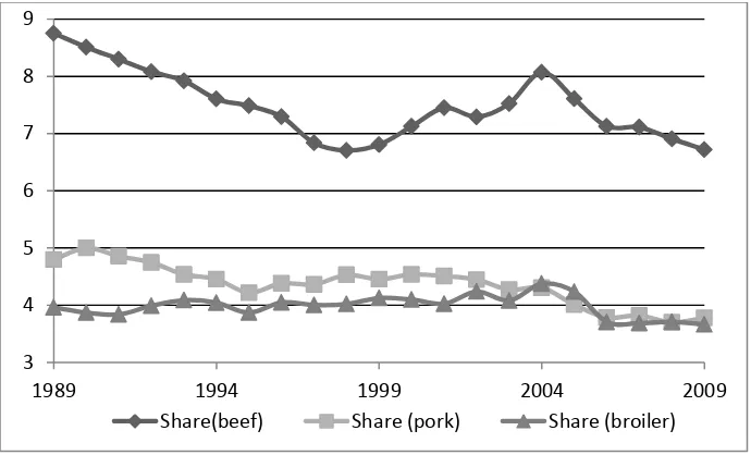
increased from 1.3 in 1989 to 1.7 in 2007. The second factor is the change in consumers’
preferences away from red meats and towards the white meats, predominantly due to
consumers’ health concerns. The expenditure shares of various meat categories depicted in
Figure 5 illustrates the point.
Besides the higher per capita consumption and the population growth, the other
contributing factor for the expansion of the broiler industry’s production came from exports.
As seen in Figure 6, from 1987 to 2007 the U.S. broiler exports increased approximately 7
times, from less than 1 billion pounds to nearly 7 billion pounds. There are multiple reasons
for the increase of the U.S. broiler exports, but one of the most important reasons is that the
U.S. government started to support the U.S. broiler exports from 1991 onward4.
After the introduction of this export support program, the U.S. has made substantial
increases in the volume and value of the broiler exports to various countries all around the
world. For instance, the U.S. broiler exports to Russia increased from in 1989 to 1.89
billion pounds in 2007. In fact, Russia surpassed Hong Kong and became the largest
importing country of the U.S. broiler since 1994. As the second largest U.S. broiler importing
country in 2007, mainland China increased its imports of the U.S. broiler from 0.68 million
pounds in 1989 to 650million pounds in 2007. Hong Kong also made a contribution to the
growth of the U.S. broiler exports. Its import of the U.S. broiler increased from 0.21 million
pounds in 1989 to 970 billion pounds in 1995 (it peaked in 1995 and then started to decline).
Other countries such as Mexico and Canada increased their imports of U.S. broiler as well
during the period. Mexican imports of the U.S. broiler increased from 90 million pounds in
1989 to 534 million pounds in 2007. Canada imports of the U.S. broilers increased from 63
million pounds in 1989 to 251 million pounds in 2007.
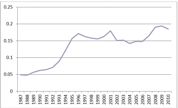
The ratio of exports to U.S. total production also increased from 4.87% in 1987 to
18.52% in 2010 (see Figure 7). Strong reliance on exports, together with various trade
barriers that effectively blocked the imports of fresh and chilled chicken meat from low cost
producing countries (e.g. Brazil) was essential for industry profitability and overall success.
Domestic consumers’ strong preference for white (breast) meat and the lack of demand for
dark meat (leg quarters) forced the U.S. broiler industry to look to overseas markets to get rid
of large quantities of leg quarters (Rabobank, 2011).
2.3 Industry Structure and Dynamics
During the same period (1992 to 2007), the broiler industry has become more and more
concentrated as a result of mergers and acquisitions. The Herfindahl index (HHI) of poultry
processing industry increased from 735 to 1224 from 1992 to 2007.5 The industry's Top-4
concentration ratio increased from 44.24% in 1992 to 58.52% in 2007, and Top-8
concentration ratio increased from 60.30% to 72.14%.6 For comparison purposes, the rest of
the meat complex in the U.S. is even more concentrated with beef and pork industries’
concentration ratios exceeding that of the broiler industry. In 2007, the 4-firm concentration
ratio for beef was about 80%, and for pork about 68% compared to only 58.52% for broilers.
5
In the calculation of HHI I picked the top 50 firms and left the rest of firms in the “other” category with Census data of Manufacture.
6 Top-4 and Top-8 are the top 4 firms’ market shares and top 8 firms’ market shares in the value of shipments
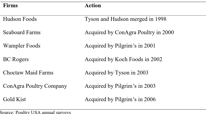
Table 2 lists the most significant mergers and acquisitions that happened among the
leading 25 broiler firms from 1997 to 2009. As a general tendency, most acquiring firms are
large firms while most acquired firms are small firms. The exception to this is Gold Kist7
whose position was No.3 when it was acquired by Pilgrim’s Pride8 who was then No. 2.9
The Pilgrim’s Pride’s case is compelling: after a series of aggressive acquisitions
(Wampler Foods Inc. in 2001, ConAgra Poultry Co. in 2003, and Gold Kist in 2006),
Pilgrim’s filed for Chapter 11 bankruptcy protection on December 1, 2008, because of the
deterioration of poultry pricing combined with an increase in input costs and the company's
lack of liquidity to withstand the downturn10. According to The Wall Street Journal
(February 12, 2009), the company terminated the contracts with at least 300 growers in
Arkansas, Florida and North Carolina because Pilgrim stopped or reduced production at
processing plants in those areas.
Despite several activities in the mergers and acquisitions area in the broiler industry, the
rankings of the leading players remained relatively stable during the analyzed period (see
7
While some of the statistical/econometric analyses in this research employ confidential Census microdata, the reference to this company by name is based on information that comes solely from an external trade publication Watt Poultry USA (various issues) and does not imply anything about whether that company is in (or not in) any data samples constructed using the Census microdata.
8
While some of the statistical/econometric analyses in this research employ confidential Census microdata, the reference to this company by name is based on information that comes solely from an external trade publication Watt Poultry USA (various issues) and does not imply anything about whether that company is in (or not in) any data samples constructed using the Census microdata.
9
Pilgrim’s sent an unsolicited proposal to Gold Kist offering to purchase all of the outstanding shares for $20.00 per share in cash on 18 August, 2006. The agreement was reached on 4 December 2006 at the price of $1 higher than Pilgrims’ initial offer.
10Pilgrim's Pride successfully emerged from bankruptcy protection on December 28, 2009 after 64% of its
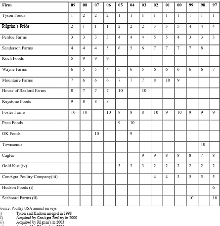
Table 3). Tyson11 was and remained the number one U.S. broiler company, except briefly in
the 2006-2008 period when its number one position was taken over by Pilgrim’s. The other
two large players are Perdue Farms and Sanderson Farms. Perdue represents an interesting
case because it is the only privately-owned large company in this market segment which is
dominated by publicly held companies. Table 4 shows that the production shares of most
broiler companies were stable over the time period except Pilgrim. Pilgrim’s production
increased from 6.40% in 1997 to 18.90% in 2009, peaking at 24.78% in 2006, because
Pilgrim conducted a series of aggressive acquisitions during the time period.
2.4 Today’s Industry
The overall positive economic outlook of the U.S. broiler industry changed dramatically
with the recession of 2008, and the long-term industry outlook became rather uncertain. In
the last several years, the US broiler industry has been facing unprecedented challenges. The
most serious challenge comes from the high cost of feed. There are several reasons for a
sharp rise in prices of corn and soybeans, including increasing livestock and poultry
production in emerging markets caused by increased demand for protein diets and domestic
ethanol subsidies. Secondly, the US domestic market is maturing, and the international
competition is intensifying. As seen in Figure 2, the U.S. per capita consumption of broilers
has been decreasing since 2006 and similar trends characterize other meats. The weakening
of the demand for U.S. poultry in once traditional export markets such as Russia (mainly due
to increased Russia domestic production) and the stiffer competition from the low cost
11
producers (such as Brazil) require the broiler companies to rethink their production strategies
and perhaps reduce production.
More consolidation is probably on the way with mergers and acquisitions targeting other
protein segments becoming increasingly likely. The companies that participate in all protein
markets (chickens, pork and beef) simultaneously (such as JBS and Tyson) are probably the
way of the future. Those who do not recognize the change in the operating environment and
change their strategies may not survive and may eventually leave the industry.
Table 1: Growth in Broiler Production (%), 1987-2007
Year Range 1987-1992 1992-1997 1997-2002 2002-2007
Broiler production growth rate 35.62 29.36 17.94 12.16
Contributions from growth in:
Population 5.80 6.24 5.60 4.77
Per Capita Consumption 18.88 9.01 12.89 5.67
Other (mainly exports) 10.94 14.11 -0.55 1.72
Table 2: Major Mergers and Acquisitions among Top 25 firms, 1997- 200912
Firms Action
Hudson Foods Tyson and Hudson merged in 1998
Seaboard Farms Acquired by ConAgra Poultry in 2000
Wampler Foods Acquired by Pilgrim’s in 2001
BC Rogers Acquired by Koch Foods in 2002
Choctaw Maid Farms Acquired by Tyson in 2003
ConAgra Poultry Company Acquired by Pilgrim’s in 2003
Gold Kist Acquired by Pilgrim’s in 2006
Source: Poultry USA annual surveys
12
Table 3: National Rankings of Broiler Companies, 1997-200913
Firm 09 08 07 06 05 04 03 02 01 00 99 98 97
Tyson Foods 1 2 2 2 1 1 1 1 1 1 1 1 1
Pilgrim’s Pride 2 1 1 1 2 2 2 3 3 5 4 4 4
Perdue Farms 3 3 3 3 4 4 4 5 5 4 3 3 3
Sanderson Farms 4 4 4 5 6 5 6 7 7 7 7 8
Koch Foods 5 9 9 9
Wayne Farms 6 5 5 4 5 6 5 6 6 6 6 6 7
Mountaire Farms 7 6 6 6 7 7 7 8 10 9
House of Raeford Farms 8 7 7 7 10 10
Keystone Foods 9 8 8 8
Foster Farms 10 10 10 8 8 8 10 9 10 9 9 9
Peco Foods 9 10
OK Foods 10 9
Townsends 10
Cagles 9 9 8 8 8 7 8
Gold Kist (iv) 3 3 3 2 2 2 2 2 2
ConAgra Poultry Company(iii) 4 4 3 5 5 5
Hudson Foods (i) 6
Seaboard Farms (ii) 10 10
Source: Poultry USA annual surveys
(i) Tyson and Hudson merged in 1998
(ii) Acquired by ConAgra Poultry in 2000
(iii) Acquired by Pilgrim’s in 2003
(iv) Acquired by Pilgrim’s in 2006
13 While some of the statistical/econometric analyses in this research employ confidential Census microdata, the reference to this company
Figure 1: US Broiler Production (million lbs), 1987-2010 Source: USDA-ERS all meat supply and disappearance data
Figure 2: Meat Consumption per Capita (lbs), 1987-2010 Source: calculated from USDA-ERS all meat supply and disappearance data
40 45 50 55 60 65 70 75 80 85 90
1989 1994 1999 2004 2009
Figure 3: Meat Real Retail Prices (dollars/lb), 1989-2009 Source: USDA-ERS all meat prices
0.5 0.7 0.9 1.1 1.3 1.5 1.7 1.9 2.1 2.3 2.5 19 89 19 90 19 91 19 92 19 93 19 94 19 95 19 96 19 97 19 98 19 99 20 00 20 01 20 02 20 03 20 04 20 05 20 06 20 07 20 08 20 09
Figure 4: Retail Prices of Beef and Pork Relative to Broilers, 1989-2009 Source: USDA-ERS all meat prices
Figure 5: Expenditure Shares of Meat on Food Expenditure (%), 1987-2009
Source: calculated from USDA-ERS all meat prices and USDA-ERS all meat supply and disappearance data
3 4 5 6 7 8 9
1989 1994 1999 2004 2009
Figure 6: US Broiler Exports (million lbs), 1987-2010 Source: USDA-ERS all meat supply and disappearance data
Figure 7: US Broiler Export Ratio in Values (%), 1987-2010 Source: calculated from USDA-ERS all meat supply and disappearance data
CHAPTER 3: WELFARE EFFECTS OF THE HORTIZONTAL CONSOLIDATION IN THE BROILER INDUSTRY14
3.1 Introduction
The U.S. poultry industry in general, and particularly the broiler industry, is often considered
the role model for the industrialization of agriculture. The poultry industry is one of the most
integrated agricultural industries. It has dominated the competitive scene in the meat complex
over the last 30 years, expanding its market share dramatically as it improved efficiency,
maintained lower prices than its competitors, and improved its product offerings and variety.
Overall, the poultry industry's vertical integration and reliance on production contracts with
independent farmers undoubtedly facilitated the industry’s efficiency and responsiveness to
consumers, making it a more formidable competitor in the global meat market (Tsoulouhas
and Vukina 2001).
The broiler industry is entirely vertically integrated, from breeding flocks and hatcheries
to feed mills, transportation divisions and processing plants. The finishing stage of
production is organized almost entirely through contracts with independent growers. A large
proportion of the value added in processing is the main reason the processors became the
coordinators of the industry, whereas the significant economies of scale in processing have
led to a significant industry concentration.
This concentration coupled with restructuring occurred either through the replacing of
existing plants with fewer, larger, more efficient ones, or through reorganization and
14 Any opinions and conclusions expressed herein are those of the author(s) and do not necessarily represent the
consolidation of assets of existing firms into more efficient configuration, or both. The
concentration and restructuring in the poultry industry could have two impacts: (a) social
welfare would decrease because higher concentrated industry means higher market power (b)
social welfare would increase because the industry restructuring may improve cost
efficiency. The objective of the chapter is to determine which one of the two effects
dominates. In other words, are the cost reductions (synergies) through consolidation enough
to offset the allocation inefficiency resulting from greater market power?
The results of this paper show that Herfindahl-Hirschman Index (HHI) increased in the
periods between 1992-1997 and1997-2002, and decreased in the period 2002-2007.
Consumer surplus increased in all three periods. Producer surplus is positively correlated
with HHI; that is, producer surplus increases when HHI increases and decreases when HHI is
decreases. The overall social welfare increased during the HHI increased period (1992-2002),
while decreasing during the HHI decreasing period (2002 to 2007), which means the society
benefited from higher concentration in the poultry industry.
The rest of this chapter is organized as follows. Section 2 reviews the relevant literature,
both theoretical and empirical. The empirical methodology is detailed in Section 3. Section 4
describes the data. Results are reported and discussed in Section 5 and the final Section
concludes the chapter.
3.2 Literature review 3.2.1 Theoretical Literature
The theoretical literature in this area starts with Williamson (1968) who first modeled the
for computing the average cost reduction necessary to neutralize the allocation inefficiency
of post consolidation rise in output price. Williamson (1968) argued that if the post-merger
price decreased, the social welfare would certainly increase. This is because when the price
decreases, the total output should increase, and the consumer surplus would certainly
increase. On the other hand, because merged firms produce more with lower average cost
( because mergers shift the merged firm’s average cost and marginal cost function down), the
non-merged firms produce less with the lower average cost (the non-merged firms’ average
cost and marginal cost functions do not shift; this change is along the average cost curve). As
a result, the model predicts that the industry average cost will decrease, and the overall
industry production will increase, which consequently increases the producer surplus. In the
case of an increase in the post-merger price, the results are ambiguous. The welfare tradeoff
model applies most easily to the case of two firms that merge into a monopoly. The analysis
recognizes that in the case of a demand curve that is relatively elastic, the efficiency gains
from a cost-reducing merger (toward monopoly) could easily outweigh the incremental
deadweight loss from the post-merger monopoly pricing. Williamson (1968) provided the
core theoretical basis used today for taking efficiencies into account in horizontal merger
analysis.
The Department of Justice’s “Merger Guidelines” (1984) takes Williamson’s
trade-off explicitly into account. The main focus is on market concentration typically measured by
the HHI. The HHI is calculated by summing the squares of the individual market shares of all
the participants. Compared to the top-4 firms’ concentration ratio, the HHI reflect both the
that will not result in a highly concentrated market (HHI greater than 1000) or increase
concentration by very much (less than 100 points or 50 points) will be permitted without
further investigation. For the mergers which cross the threshold, the Department of Justice is
likely to challenge them. The Department will not challenge the merger if it produces
significant cognizable efficiencies which cannot be achieved by the parties through other
means. “Cognizable efficiencies include, but are not limited to, achieving economies of scale,
better integration of production facilities, plant specialization, lower transportation cost, and
similar efficiencies relating to specific manufacturing, servicing, or distribution operations of
the merging firms” (Guidelines 1984). When these cognizable efficiencies are large enough
to offset the price increase as a result of market power increased by the potential merger, the
merger is likely to be permitted.
Because the Guidelines (1984) focus on whether output price increases or decreases,
recent papers focus on the effect of mergers on price. The measured effect is unilateral
because researchers assume that non-merging rivals do not alter their strategies either
pre-merger or post-pre-merger. In this case, if the price does not increase after the pre-merger, social
welfare will definitely increase. In other words, no increase in price is the sufficient condition
for social welfare to increase.
Farrell and Shapiro (1990) derived the necessary condition to maintain the price before
and after the merger. They show that the post-merger price will decrease if and only if the
price cost margin of the merged firm is larger than the sum of the price cost margins of the
merge firms when the merged firm produces at the level of total production of the
decreases significantly to offset the effect of higher post-merger market power. Farrell and
Shapiro (1990) also relate the marginal cost of the merged firm to the share of the pre-merger
firms, demand elasticity and pre-merger price. They showed that larger pre-merger firms and
lower demand elasticity require more cost reduction to prevent price from increasing after
merger. This result is reflected in the Horizontal Merger Guidelines (1997) which recognizes
that the greater the potential adverse competitive effect of a merger (as indicated by the
increase in the HHI and post-merger HHI), the greater must be the cognizable efficiencies in
order for the merger not to have an anticompetitive effect in the relevant market.
Farrel and Shapiro (1990) further extend their model to general cost and demand
functions. They argue that because it is hard to compare pre- and post-merger allocations
directly, they studied the merger effect on the welfare of non-merging firms and consumers,
which they called external welfare effects. Because the profit of merged firm should increase
after merger (otherwise the firms would have not merged to begin with), if the welfare of
non-merging firms and consumers increase as a result of the merger, social welfare will
increase for sure. Farrel and Shapiro (1990) also showed that if the market share of the new
firm is less than the sum of the market shares of the other firms in the industry weighted by
their respective conjectural variation terms, external welfare effects will be positive.
Werden and Froeb (1998) derived the ratio of marginal cost reduction to pre-merger
price needed to prevent the price from increasing after a merger as a function of the
pre-merge market shares and demand elasticity. Their result is quite similar to Farrell and
(in absolute value), the more reduction in marginal cost is required to prevent the
post-merger price from increasing.
As said earlier, having no increase in the post-merger output price is a sufficient
condition for social welfare to increase. However, the social welfare could increase even
when the post-merger price goes up if the increase in producer surplus dominates, i.e. when
cost synergies are substantial. Although the studies by Farrell and Shapiro (1990) and its
extensions are widely accepted by economists, the Horizontal Merger Guidelines (2010) are
still in favor of protecting competition and consumer surplus.
3.2.2 Empirical Literature
Different consequences of mergers and acquisitions have been studied empirically. Some
authors study the effects of mergers on the partners’ profitability (Cosh, Hughes & Singh,
1979; Kumar, 1985; Meek, 1977; Ravenscraft and Scherer, 1987; Utton,1974). Others study
the relationship between ownership change and the stock market performance (Alberts &
Varaiya, 1989; Hughes, 1993; Mueller, 1989; Roll, 1986 . Other studies are concerned with
productivity and prices. Since the literature in this field is huge, this review will focus only
on the empirical studies in food and beverage and meat packing industries.
The first group of studies looks into the effect of mergers and acquisitions on
productivity. The main finding of this literature is that mergers and acquisitions will increase
productivity, as shown by Lichtenberg and Siegel (1992) and McGuckin and Nguyen (1995),
among others. On the other hand, Nguyen and Ollinger (2006) argue that Lichtenberg and
Siegel’s (1992) and McGuckin and Nguyen’s (1995) results may not hold for more narrowly
industry, sausages and other prepared meat product industry as well as the poultry
slaughtering and processing industry) before and after mergers using 1977-82 and 1982-97
periods. Their results show that smaller acquired plants in the meat packing industry,
sausages and other prepared meat product industry and larger plants in the poultry
slaughtering and processing industry in 1977-87 improved their productivity growth after
merger. But for smaller plants of the poultry processing industry during 1982-87 and all
plants of poultry processing industry during 1987-92, there was no improvement in
productivity.
Other researchers studied the effect of mergers and acquisitions on employment and
wages with different results obtained by using different data. Brown and Medoff (1988),
using a sample of firms in Michigan, found that mergers and acquisitions have little effect on
employment and wages. But Lichtenberg and Seigel (1992) found that mergers and
acquisitions of manufacturing plants led to reduction in both employment and wages at
central offices but had little effect at production establishments. Further,, McGuckin and
Nguyen (1998) showed that the change in ownership increased the wages of employees of
acquired plants by 12% and employment by 16% in food industry over 1977-82. Nguyen and
Ollinger (2007) showed that mergers and acquisitions increased wages in the meat packing
and prepared meat product industries over 1977-87 but not during 1982-92, and it resulted in
increased employment in all three meat and poultry industry over 1977-87 period, but only in
poultry for 1982-92.
Yet other studies focused on the effect of mergers and acquisitions on input price, output
lead to lower input prices (Wald, 1981; Menkhaus et al., 1981; Hayenga, Deiter and
Montoya, 1986; Menkhaus, Whipple and Ward, 1990; Ward, 1992). On the other hand, the
results for the effect of higher concentration on margins vary. Schroeter and Azzam (1990)
and Brester and Musick (1995) found higher industry concentration was associated with the
higher farm-to-wholesale marketing margins in the beef and pork packing industries and
higher farm-to-retail margins in the lamb industry. Matthews (1999) used monthly data from
1979 to 1996 and found no significant association between increased concentration and
farm-wholesale marketing margins. Ward and Stevens (2000) also found little aggregate effect in
the beef industry price linkages resulting from increased packer concentration.
Finally, the Williamson welfare tradeoff due to consolidation in the beef packing
industry was studied by Azzam and Schroeter (1995). The objective was to determine what
cost reductions are necessary to offset the anticompetitive effects of market power resulting
from consolidation in a regional oligopolistic industry. He found that the unit costs would
have to decrease by 0.29% to neutralize the effects of a 50% increase in concentration, and
would have to decrease by 2.94% to offset the effects of a cartelization of the buyers’ side of
the cattle market.
3.3 Empirical Methodology 3.3.1 Producer Surplus
3.3.1.1 Cost Function Estimation
In order to calculate the producer surplus, I first estimate the cost function for the U.S. broiler
industry. We use the generalized Leontief cost function, first introduced by Diewert and
(1). ∑ ∑ ∑ ∑ ,
where is output cost for plant , is price of input for plant , and is the output
quantity for plant ,. s and s are the parameters to be estimated. With the generalized
Leontief cost function, homotheticity is satisfied by construction. I impose the restriction
such that the symmetry condition is also satisfied. When and ,
the underlying production function from which (1) is derived has the property of constant
returns to scale (CRS).
Appling Shephard’s Lemma to (1) gives the input demand functions,
(2). ∑ ,
where is the quantity demanded of input for plant . In order to convert the theoretical
model (2) to an empirical model, I append errors to (2):
(3). ∑ ,
where s are error terms. The equation system is then estimated by iterated seemingly
unrelated regression (ITSUR). The following paragraphs show how ITSUR estimate
parameters. We now rewrite (3) in terms of matrix to make the explanation easier to
understand:
where [
], is a parameter vector, is matrix of independent
variables, [
]. In ITSUR, , , and are assumed to be correlated. But
and are independent with each other for . Parameters are then estimated by feasible generalized least squares. Because the variance-covariance matrix of s (name it ) is
unknown, we need to estimate the parameters by iteration. In the first step, we run ordinary
least squares for (4). The residuals from this regression are used to estimate elements of . In
the second step, we run the generalized least squares regression for (4) to get the second
estimation of . The residuals from this second regression can be used to form the second
estimator of . The estimation runs iteratively until the convergence is achieved. In order to
account for changes in the cost function across time, we estimate the equation system (4) for
each census year separately. We assume that the changes in cost function parameters across
different years are caused by changes in industry concentration. After estimate parameters,
from equation (3), we can calculate the input demand elasticities by formulas below:
(5). ∑ ̂
̂ ∑ ̂ ̂ ̂
,
(6). ̂
̂ ∑ ̂ ̂ ̂
,
where is own price elasticity for input , is cross price elasticity for input with respect
From equations (5) and (6), we can see that and will change with different s, s
and s. So we substitute the industry averages of input prices, output quantities into the
equations to get the elasticities:
(7). ∑ ̂ ̅̅̅̅ ̅̅̅̅ ̅ ̅̅̅̅
̂ ∑ ̂ ̅̅̅̅ ̅̅̅̅ ̅ ̂ ̅̅̅
(8). ̂ ̅̅̅̅ ̅̅̅̅ ̅ ̅̅̅̅
̂ ∑ ̂ ̅̅̅̅ ̅̅̅̅ ̅ ̂ ̅̅̅
,
where ̅̅̅̅ s , ̅ are industry average of input prices and output quantiy.
3.3.1.2 Producer Surplus
With the cost function estimated out, we can compute the producer surplus for each plant
in each census year as follows:
(9). ∫ ( ) ,
where denotes the producer surplus, is the total revenue and ( ) is the marginal cost function. ( ) can be obtained by taking the partial derivative of (1) with respect to the output quantity and takes the following form,
(10). ( ) ∑ ∑ ∑ .
Using (10), (9) can be rewritten as,
(11). ∑ ∑ ∑ ,
where is the price of input for plant in year and the parameters have a subscript
because as mentioned above, we estimate the cost function for each census year separately.
across all plants in that year, that is, ∑ , where is the number of plants in
census year .
With the method above, we implicitly assume that the changes in producer surplus
across different census years are caused only by changes in industry concentration. Industry
concentration could affect the producer surplus in many different ways: First, in the output
market, broiler processing firms could have higher oligopoly power could charge higher
prices to consumers. Second, in the input markets, broiler processing firms having higher
oligopsony power to procure inputs at a lower price (that is, lower in (1)). Third, larger
firms could have higher incentives and more funding for research and development in
technological improvements which could potentially lower the marginal cost. There are other
factors that could potentially cause changes in the producer surplus across different census
years, not including them in this analysis. For example, changes in the supply and demand
conditions in the grain market can cause changes in the feed price (hence changes in for
materials in (1)) and hence the cost and the producer surplus. While a higher concentration
rate of broiler processing firms would increase their ability to negotiate the price of live
chicken, this not not likely to be the case with other input makets. One way to address this
problem is to fix prices for labor, energy and capital, while allowing prices for material to
3.3.2 Consumer Welfare15
3.3.2.1 Estimating Demand for Chickens
To calculate changes in consumer surplus due to changes in industry concentration, we first
need to estimate consumers’ demand for meats including beef, pork and chicken. We use the
almost ideal demand system (AIDS) model introduced by Deaton and Muellbauer (1980).
The system consists of demand equations for beef, pork, poultry, and other (food and
nonfood) consumption items16. Inclusion of The inclusion of an equation representing
consumption of “all other goods” (food and non-food) and use of per capital total personal
consumption expenditures as the income variable implies that we are estimating
unconditional demand system instead of conditional demand system17.
The AIDS model starts with the following expenditure function for a representative
consumer:
(12). ( ) ( ) ( ),
where ( ) ∑ ∑ ∑ , ( ) ∏ , is the price for good and s, s and s are parameters to be estimated.
15 I want to appreciate Michael Wohlgenant’s guidance and help in this part: including the suggestion of
demand estimations (use unconditional demand system instead of conditional demand system), seasonal dummies and calculation of compensating variations as an alternative measure of consumer welfare.
16 LaFrance and Hanemann (1989) proved in their paper that incomplete demand systems are weakly integrable
if the incomplete demand systems are augmented with an artificial composite commodity representing “other goods”. And they also showed that the exact welfare measures can be obtained from directly from any weakly integrable set of demand functions.
17 Hanemann and Morey(1992) showed in his paper that even with the assumption of separability, the partial
Applying the Shephard’s Lemma to (12) yields the following demand system,
(13). ∑ ( ) for all ,
where is the expenditure share of good , is the price index, that is, ( ) and is the representative consumer’s budget for meat consumption. For estimation purposes, the
AIDS model is often re-formulated as the LA/AIDS model by replacing the price index using the Stone index:
(14). ∑ .
The resulting LA/AIDS model is simpler and it makes the estimating equation (13) linear in
parameters. Moschini (1996) shows that the Stone index is not invariant to price scaling and
recommends using price indices instead of actual prices. This means we need to normalize
each price series in (13) such that the price of each good takes the value of one in the base
period.
To take into account of the year, seasonal shocks in meat consumption, we include time trend
and quarter dummies in (14):
(15). ∑ ( ) ( ) for all ,
where the subscript is added to the variables to denote the time period, the variable is the
time trend, s are the quarterly dummy variables and is an error term appended to the
equation to turn the theoretical model (13) into an empirical model (15). To avoid the
where ̅ is the average share of good across different time periods. Also, to address the possible autocorrelations in the error term , we take the first difference of (15).
(16). ∑ ( ) ( )
for all ,
(16) is the final empirical demand system model we estimate. We impose the following set of
restrictions, ∑ , ∑ ∑ , ∑ and such that the demand system satisfies the homogeneity and symmetry conditions, as required by the demand
theory. This demand system is then estimated by ITSUR as well.
3.3.2.2 Change in Consumer Surplus18
To compute the change in consumer surplus due to changes in industry concentration in the
broiler processing industry, we need to derive the demand function for chicken from the
AIDS model. By definition, the expenditure share for chicken is:
(17). 𝑐 𝑝𝑐 𝑞𝑐 𝑐 𝑐 ∑ 𝑐 ( )
𝑐 ( ) 𝑐 ,
where the subscript denotes chicken. Therefore:
(18). 𝑞𝑐 𝛼𝑐 𝜃𝑐 𝑑 𝑄 𝑑 𝑄 𝑑 𝑄 ∑ 𝛾𝑐 𝑜𝑔(𝑝 ) 𝑐 𝑜𝑔 ( 𝑒 𝑃 )
= 𝑐
𝑝𝑐 ,
and the consumer surplus is:
18 LaFrance and Hanemann (1989) noted in their paper that the consumer surplus line integral is not unique and
(19). 𝑐 ∫ 𝑞p𝑐 𝑐 ( 𝑐 ) 𝑐
+
𝑝𝑐 ,
where 𝑐 is the price of chicken in period and 𝑐 is the price of chicken when zero amount
is consumed. For 𝑐 , we use the yearly broiler price from USDA for year .
Computing 𝑐 , is more involved. Let 𝑐 ( 𝑐 𝑐
∑ 𝑐 ( ) 𝑐 ( ) 𝑐∑ ̅ ( ) 𝑐 ) and 𝑐 ( 𝑐𝑐 𝑐̅̅̅)𝑐 , then
(18) can be rewritten as
(20). 𝑞𝑐 ( 𝑐 ) 𝑐 𝑐 𝑝 𝑜𝑔 (𝑝𝑐 )
𝑐 .
When 𝑐
𝑐
𝑐 , 𝑞𝑐 ( 𝑐 ) . As a result, one may conclude that 𝑐 𝑐 𝑐 is the choke
price for chickens. But this conclusion might be incorrect because this result does not take
the shape of the demand curve into account. To learn more about the shape of the demand
curve, we take the partial derivative of the demand function for chicken with respect to the
price of chicken:
(21). 𝑞 𝑝𝑐 (𝑝𝑐 )
𝑐
𝑐
𝑝𝑐
𝑐 𝑐 𝑜𝑔(𝑝𝑐 )
𝑝𝑐
𝑐 𝑐 𝑜𝑔(𝑝𝑐 )
𝑝𝑐
By setting (21) equal to zero, we see that when 𝑐
𝑐
𝑐 , 𝑞𝑐 ( 𝑐 ) attains its extreme
value (the extreme value is 𝑐
𝑐
𝑐 ). Whether this value is a maximum or a minimum
depends on the sign of the second derivative of the demand function evaluated at the extreme
value. The second derivative of the demand function with respect to price is:
(22). 𝑞 𝑝𝑐 (𝑝𝑐 )
𝑐
𝑐 𝑐 𝑐 𝑜𝑔 (𝑝𝑐 )
Evaluating (22) at 𝑐
𝑐
𝑐 yields 𝑞𝑐 (𝑝𝑐 )
𝑝𝑐
𝑐
𝑝𝑐 . So if 𝑐 is negative, which means
that the demand for chicken is elastic, the extreme value is a minimum. If 𝑐 is positive,
which means that the demand for chicken is inelastic, the extreme value is a maximum. The
two cases are illustrated in Figures 3.1 and 3.2.
Therefore, when 𝑐 , 𝑐
𝑐
𝑐 . But, as we can see from Figure 3.1, when
𝑐 ,
𝑐
𝑐 is not the real choke price because for prices above 𝑐 𝑐 , the quantity will
decrease but will never go to zero again. In other words, there is no real choke price when
𝑐 . This implies that when demand is inelastic, 𝑐 , the consumer surplus will be
positive infinity as well. So we could only calculate the change in consumer surplus instead
of the absolute value of consumer surplus. The change in consumer surplus between two
years could be expressed as:
(23). 𝑐 𝑐 𝑐 ∫𝑝 𝑞𝑐 ( 𝑐) 𝑐
𝑐 ∫ 𝑞𝑐 ( 𝑐) 𝑐
𝑝𝑐
where 𝑐 is the chicken price in year and 𝑐 is the chicken price in year .
From (23), it is clear that there are two sources of the changes in consumer surplus
across different time periods. The first source is the change in the demand function, that is,
the demand function for chickens changes from 𝑞𝑐 ( ) to 𝑞𝑐 ( ). The second source is the change in the poultry price, that is, the price for chickens changes from 𝑐 to 𝑐 . Since we
are only interested in the consumer surplus change resulting from the change in chicken price
caused by changes in industry concentration in the broiler processing industry, we fix the
period of 1992 to 2007, we compute two versions of (23) for each pair of years, once using
the demand function for chickens in 1992 and once using the demand function for chicken in
2007. With this, (23) becomes:
(24). 𝑐 ∫𝑝𝑝𝑐 𝑞𝑐 ( 𝑐) 𝑐
𝑐 or 𝑐
∫ 𝑞
𝑐 ( 𝑐) 𝑐 𝑝𝑐
𝑝𝑐 .
Finally, note that since we use (16) to estimate the demand system, 𝑐 and 𝑐 are not
estimated. However, we need an estimate for 𝑐 𝑐 to compute the change in consumer
surplus using (24). We use the difference between the observed expenditure share for chicken
and the estimated value of the right hand side of (15) excluding the 𝑐 𝑐 , that is, (25) 𝑐̂ 𝑐 𝑐 [ ̂ 𝑐 ̂ 𝑐 ̂ 𝑐 ̂ 𝑐 ∑ ̂ ( 𝑐 )
𝑐
̂ ( )],
Where ̂ , 𝑐 ̂ , 𝑐 ̂ , 𝑐 ̂s and 𝑐 ̂ are parameter estimators. 𝑐
With the method above, we implicitly assume that the change in output price is due entirely
to change in HHI. However, a change in output price could be caused by development in the
export market. For example, a positive shock in the export market could increase price of leg
quarters (main export item). This could to decrease domestic price (for white meat), because
poultry companies always tend to cross-subsidize their export by charging higher prices for
domestic market. However, except in the first period of my study (1992 to 1997),
export-to-production ratios were fairly stable (see Figure 2.7). This indicates there is no major shock
strictly caused by HHI. From 1992 to 1997, the export ratio increased dramatically from
around 7.5% to more than 15% (more than doubled). So during this time period, increase in
consumer surplus could have been partially caused by positive shocks in the export market.
3.3.3 Compensating Variation
In fact, compensating variation (CV) is generally considered to be a better measurement of
the welfare effect on consumers than CS. CV is defined as the amount of money consumers
would pay or would need to be paid to be just as well off after the price change as they were
before the price change. In most empirical studies, because Hicksian demand is generally not
observable, CS (calculated from Marshallian demand) is used as an approximation of CV
(calculated from Hicksian demand). The primary condition for CS to be a good
approximation to CV is constant marginal utility of income. Hausman (1981) argues that in
the case of single price change no approximation is necessary to measure consumer welfare
change. In his paper, by developing a method to calculate unobservable Hicksian demand
function from observable Marshallian demand function, he was able to estimate the exact
measure of consumer welfare changes. In this part of this chapter, we follow Hausman’s
approach to calculate compensating variation. Instead of a general demand function, we
apply his approach to LA/AIDS model.
In our model, following Hausman’s approach, we rewrite (12) as,
where ( ) is the representative consumer’s indirect utility given expenditure and price vector . Let ( ) denotes the indirect utility in year . We then have the following formula for CV:
(27). ( ) ( ),
where the expenditure function ( ) is defined in (12) and is the price vector for all products in the demand system in year . We are now ready to state the following result.
Result1: When the prices for beef, pork and “all other goods” remain the same and only the price of chicken changes from 𝑐 to 𝑐 , (27) can be rewritten as follows:
(28). { { 𝑐 𝑐 𝑐𝑐( 𝑐) [ 𝑐 𝑜𝑔 𝑝𝑐 ]( )} },
where 𝑐 𝑐 𝑐 , 𝑐 𝑐 ∑ 𝑐 and
∑ ∑ ∑ .
Since we estimate our demand system using (16), is not estimated. If 𝑐 𝑐 is small, (28) can be rewritten as:
(29). { { 𝑐 𝑐 𝑐𝑐( 𝑐) } }, where 𝑐 is the expenditure share of poultry at time .
Proof: see the Appendix.
3.4 Data
3.4.1 Census data
The estimation of the cost function and the calculation of the producer surplus are based on
the data from the Census of Manufactures. Our sample consists of plants in the broiler
only interested in the producer surplus for broilers, we focus on those plants which use live
broilers (young chickens including commercial broilers) as the main input material and for
which processed broiler meat (broilers and fryers under 20 weeks of age, roasters and
capons) account for more than 90% of the output values.
Using the Census data, we created the following variables that are needed to estimate
the input demand system (3) and compute the producer surplus (11) for each plant. The
output variable ( ) is the total processed broiler meat produced (in thousands of lbs.), which
is directly available from the Census. Input quantities ( s) and prices ( s) were constructed
as follows. There are 4 inputs in broiler production: materials, labor, energy and capital.
Since one processed broiler comes from one live broilers, we use the total live broiler used in
production (in thousands of lbs.) as the quantity for materials, . The total live broilers used
in production are directly available in the Census data. The materials price, , was
computed by dividing the expenditure on materials (directly available in the Census data and
including expenditure on live broilers and boxes and other packaging materials, also in terms
of thousands of dollars) by .
The labor price, , was calculated by dividing the expenditure on production workers
(directly available in the Census data and including annual payroll and fringe benefits for
both leased and non-leased workers, also in terms of thousands of dollars) by the total
production workers’ production hours. The labor quantity, , was computed by dividing the
sum of the expenditure on production workers and non-production workers (both of which
implicit assumption here is that production workers and non-production workers have the
same average wage rate.19
The energy price, , was calculated by dividing the expenditure on electricity (directly
available in the Census data and in terms of thousands of dollars) by the quantity of
electricity used (directly available in the Census data and in terms of Kilowatts). The energy
quantity, , was computed by dividing the sum of the expenditure on electricity and fuel
(both of which are directly available in the Census data and in terms of thousand dollars) by
. The implicit assumption here is that the electricity price and the fuel price are the same
when electricity and fuel are converted into the same unit.20
The capital price, , was calculated by dividing the depreciation charges (directly
available in the Census data and in terms of thousands of dollars) by the total of value of
assets at the beginning of the year (directly available in the Census data and in terms of
thousands of dollars)21. The capital quantity, , was computed by dividing the sum of the
depreciation charges and rental payments for machines and buildings (both of which are
directly available in the Census data and in terms of thousands of dollars) by . The implicit
assumption here is that the rental rate for machines and buildings is the same as the
depreciation rate for machines and buildings the plant owns.22
19
This assumption is necessary as the Census data does not report the total hours for non-production workers.
20 This assumption is necessary as the Census data does not report the quantity of fuel used. 21
This method may not be accurate. The average of is quite different from the industry level rental price used in Chapter 4. Further improvement is needed for this part in the future.
22 This assumption is necessary as the Census data does not report how many machines and buildings a plant