On Doppler Mismatch of Linear Frequency Modulated
Waveforms in Active Sonar Applications
C. K. Sunith
Assistant Professor in Electronics, Model Engineering College, Thrikkakara, Kochi, Kerala, India
ABSTRACT: The development of an active sonar system requires knowledge of the properties of the waveforms transmitted by that system. The choice of waveform will determine the ability of the system to resolve targets in range and Doppler, and will also impact the detection capabilities of the system. . Modulating the frequency or the amplitude of the transmitted waveform and coding the waveform with a pseudo random sequence will result in an increased time-bandwidth product. Amplitude modulation, however, results in a decrease of power efficiency, and hence it is common to use frequency modulated signals. The use of Linear Frequency Modulated (LFM) waveforms has been in existence in active sonar systems for quite long. This article based on Matlab simulation focuses primarily on the Doppler sensitivity and mismatch characteristics of Linear Frequency Modulated waveforms.
KEYWORDS: Active Sonar, Matlab, Linear Frequency Modulation, Decimation, Beamformer, Chebyshev Polynomials, Matched Filter, Doppler Resolution.
I. INTRODUCTION
In order to maintain peak transmitted power, various forms of frequency modulation are typically used. These include Linear Frequency Modulation (LFM), with a transmit waveform expressed as:
s(t) = wT(t)exp[2i(f0t + ½ mt2)] (1a)
where
duration
pulse
extent
sweep
T
W
m
_
_
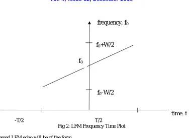
. (1b)wT is the square envelope and f0 the centre frequency. The centre frequency of the waveform was assumed 10 KHz, the bandwidth
and pulse width used were 400 Hz and 0.5 seconds respectively with a total time period of 1 second (Fig 1). For LFM, the frequency varies linearly with time as shown in Fig 2.
0 0.05 0.1 0.15 0.2 0.25 0.3 0.35 0.4 0.45 0.5 -40
-20 0 20 40
0 0.1 0.2 0.3 0.4 0.5 0.6 0.7 0.8 0.9 1 -40 -20 0 20 40 LFM WAVEFORM time a m p li tu d e
-T/2 T/2
Fig 2: LFM Frequency Time Plot
A time-compressed LFM echo will be of the form
s[(1 - )t] = wT(t)exp[2i(f0(1 - )t + ½ m(1 - )2t2)] (2)
The frequency translation term f0= - f0 is present, but in addition there is a change m= (2- 2)m in the sweep rate.
To simplify calculations and to ease implementation, it was assumed that since has a small value, 2 will be still smaller, hence (1 - )2 was approximated to 1 - 2. With this approximation, a frequency translated version of the transmitted pulse s(t) may not correlate precisely with the echo, and for m sufficiently large one must use true time-compressed references in the replica correlator .
II. RELATED WORK
Linear Frequency Modulated (LFM) waveforms and its properties for use in Radar Systems have been described in detail by Levanon et. al1, Burdick et al.2 and Winder et. al.4 in their works have explained in detail about Active Sonar Systems and the use of LFM in Active Sonar Systems. An analysis of LFM for use in Active Sonar Systems has been conducted by Glisson et. al.5 in his work. Parvana et. al.7 in their work
have conducted a performance analysis of LFM. A few mathematical expressions connected with LFM can also be found in the work by Chan et. al.8. Baldacci et. al.6 in their work have explained an Adaptive Algorithm for Normalization of Sonar Data which will be useful for future works as well. A few references can also be found online. In the proposed work, an attempt has been made to highlight one of the problems concerned with the use of LFM for Active Sonar detection.
II. SIMULATION SETUP
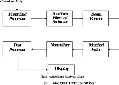
The front end processor conditions the array signal and converts it to digital signal for processing. Active Sonar receiver (Fig 3) will have to process the signal at lesser data rates. The signal is bandpass filtered to improve signal to noise ratio. Decimation process helps to sample the signal at a lesser data rate convenient to the receiver. The beamformer comprises of a series of receiving elements or hydrophones. Receiving arrays are linear assemblies of
f
0time, t
frequency, f
0f
0-W/2
hydrophone elements designed to increment signal to noise ratio and directionality. Array weights and shading coefficients are multiplied element by element with the received signal to account for the attenuation suffered, to reduce side lobe levels and improve directivity. Path difference issues between different receiving elements are resolved at this stage. Chebyshev polynomial coefficients are used as shading coefficients to suppress side lobe levels to as low as 23dB below main lobe level. A split window normaliser6 was used to estimate and remove background noise.
From Transducer Array
Fig 3 : Active Sonar Receiving Chain
IV. MATCHED FILTER RESPONSE
Matched filter response is essentially the correlation of the received signal with the stored reference. Delay Parameter tau (τ) is the round trip delay of the signal to the target and is given by:
τ = 2R0/C (3)
R0 is the range to the target and C is the sonic velocity in water whose average value is 1500 m/s. The Doppler parameter delta(δ) is given by the expression
δ = 2 V/C (4)
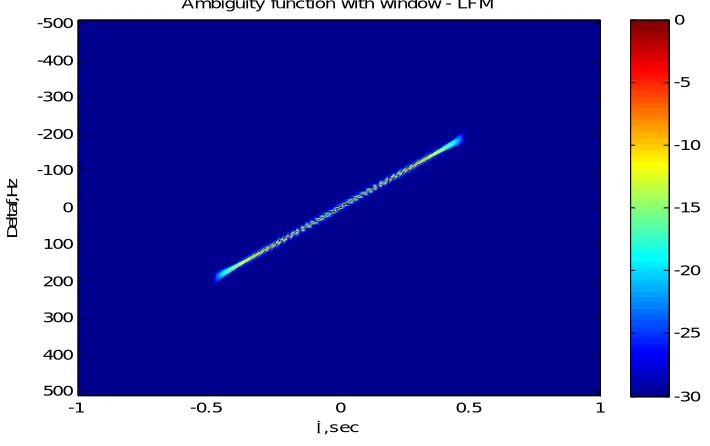
where V is the velocity of the target. The 3dB ambiguity contour1,5 of LFM plotted using Matlab is shown in Fig 4.
Front End
Processor
Band Pass
Filter and
Decimator
Beam
Former
Matched
Filter
Normalizer
Post
Processor
,sec
D
e
lt
a
f,
H
z
Ambiguity function with window - LFM
-1 -0.5 0 0.5 1
-500
-400
-300
-200
-100
0
100
200
300
400
500 -30
-25 -20 -15 -10 -5 0
Fig 4: 3dB ambiguity contour of LFM
The value of τ was maintained constantand the expected value of δ was assumed to be 0.02. The value of δ
was varied in equal steps from 0 to 0.04 and peak values of matched filter responses (Fig 5) were plotted as bar graph
V. SIMULATION RESULTS
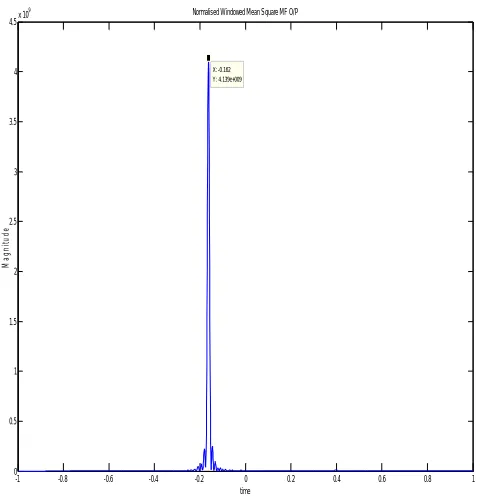
Simulations for an expected value of δ = 0.02 show that when the value of δ of stored replica (our expected signal) was set to 0.02, the matched filter response does not peak when the actual value of delta is 0.02, but instead the peak appears at a different value of δ as shown in Fig 5. This Doppler mismatch can be attributed to the approximation that was applied to equation (2), as described earlier. But when the expected value of δ for the stored replica was changed to 0.023, the matched filter response exhibited a peak at δ = 0.02. This means that the corrected value of the Doppler parameter (δ = 0.023), necessitated by the approximation made in equation (2) on stored replica of the waveform caused the matched filter output to peak when the actual value of δ became 0.02, as to exhibit a Doppler match. However, this Doppler correction applied to the value of δ to force a match was not without drawbacks. In fact the change caused a
significant reduction in the peak value as well as a change in slope and the 3dB width of the matched filter output (Fig 6a and Fig 6b) normalised6 to the rms mean of background noise. Range (R) and Doppler resolutions (V) computed for a pulse width of 0.5 second showed change in values (Table 1). With Doppler correction applied, range resolution degraded slightly, but Doppler resolution has improved. The phenomenon may be attributed to the slight change in the slope of the matched filter response as well.
Waveform R(m) V(m/s)
LFM(W.O. Correction)
2.625 21.4286
LFM(With Correction)*
3 19.5
Table 1: Range and Doppler resolution of LFM (* - Matched Filter output peak reduced)
Fig 6a: Normalised matched filter output of LFM without Doppler correction (Y Axis: Magnitude)
-1 -0.8 -0.6 -0.4 -0.2 0 0.2 0.4 0.6 0.8 1
0 0.5 1 1.5 2 2.5 3x 10
23
X: 0 Y: 2.563e+023
Normalised Windowed Mean Square MF O/P
time
M
a
g
n
it
u
d
Fig 6b: Normalised matched filter output of LFM with Doppler correction (Y Axis: Magnitude)
VI. CONCLUSIONS
Linear Frequency Modulated waveforms constitute a class of waveforms well known and widely accepted for use in active sonar applications. This paper has attempted to probe into one of the problems concerned with the use of linear frequency modulated waveforms for active sonar detection.
REFERENCES
1. Levanon, Nadav and Mozeson , Radar Signals, IEEE Press , John Wiley and Sons.
2. Burdick, W S, “Underwater Acoustic System Analysis”, Prentice Hall, Eaglewood Cliffs, NJ, 1984,ISBN 0-13-936716-0. 3. Toomay, J C, “Principles of Radar”, Prentice Hall of India, New Delhi, 2nd Edition, ISBN No. 81-203-2509-5.
4. Winder, Alan A, Sonar System Technology, IEEE Transactions on Sonics and Ultrasonics, Sept 1975.
5. Glisson, Black and Sage, On Sonar Signal Analysis, IEEE Transactions on Aerospace and Electronic Systems, January 1970. 6. Baldacci, Alberto & Haralabus, Georgios, Adaptive Normalisation of Sonar data, NURC-PR-2006-13, August 2006. 7. Parvana, Shruti and Dr. Kumar, Sanjay, “ Analysis of LFM and NLFM Waveforms and their Performance Analysis”,
International Research Journal of Engineering and Technology, Volume :02, Issue:0 2, May 2015, pp:334-339.
8. Chan, Y K, Chua, M Y and Koo, V C, “Sidelobes reduction using simple two and tristages Nonlinear Frequency Modulation”, Progress in Electromagnetic Research, PIER 98, 2009, pp:33-52.
9. http://www.radartutorial.eu. 10. http://www.uio.no.
11. https://www.ncbi.nlm.nih.gov.
12. http://www.wikipedia.com.
-1 -0.8 -0.6 -0.4 -0.2 0 0.2 0.4 0.6 0.8 1
0 0.5 1 1.5 2 2.5 3 3.5 4 4.5x 10
9
X: -0.162 Y: 4.139e+009
Normalised Windowed Mean Square MF O/P
time
M
a
g
n
it
u
d
BIOGRAPHY