ABSTRACT
QIAN, HUI. Numerical Simulations of Internal Waves Generated by Flow over a Ridge. (Under the direction of Dr. Ping-Tung Shaw).
Numerical Simulations of Internal Waves Generated by Flow over a Ridge
by Hui Qian
A thesis submitted to the Graduate Faculty of North Carolina State University
in partial fulfillment of the requirements for the Degree of
Master of Science
Marine, Earth and Atmospheric Sciences
Raleigh, North Carolina2010
APPROVED BY:
________________________ ________________________ Dr.Gerald S.Janowitz Dr. Ruoying He
_______________________________ Dr. Ping-Tung Shaw
BIOGRAPHY
ACKNOWLEDGMENTS
I would like to thank the faculty and staff in the department of Marine, Earth and Atmospheric Sciences, who afforded me opportunities to work and study. I would like especially to thank my adviser Dr. Ping-Tung Shaw for the professional instructions and step-by-step guidance over the past two years. I would like to thank my committee members Dr. Ruoying He and Dr.Gerald S.Janowitz for their insightful comments and suggestions on my research. Also, thanks go to my family, especially to my husband, Yizhen Li who supports me all these years and my son Dennis, who has made my life in the United States more colorful.
TABLE OF CONTENTS
LIST OF TABLES... v
LIST OF FIGURES ... vi
1. Introduction... 1
1.1 Characteristics of internal waves and internal solitary waves ... 1
1.2 Energy flux of internal waves... 3
2. Model description and experiments... 7
3. Model Results ... 11
3.1 Internal wave generation... 12
3.2 Dependence of internal wave energy on the topographic width... 14
3.3 Dependence of internal wave energy on barotropic current amplitude ... 16
3.4 Dependence of internal wave energy on stratification... 17
3.5 Effects of ridge height on internal wave energy ... 18
4. Parameterization of energy flux... 19
4.1 Dependence of non-dimensional energy flux on the slope parameter... 19
4.2 Energy flux from observations ... 22
5. Discussion... 24
6. Conclusions... 27
REFERENCES ... 30
Tables……….35
LIST OF TABLES
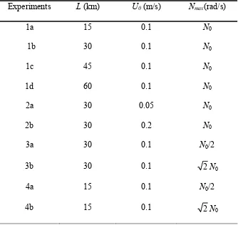
Table 3.1 List of experiments for ridge height h0 = 400 m. Experiments
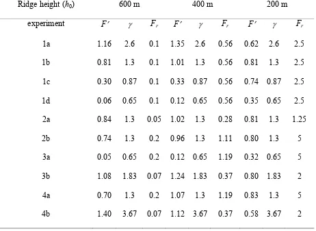
with the same parameters are repeated for ridge heights 200 m and 600 m………...35 Table 4.1 Nondimensioanl parameters calculated from all experiments in this
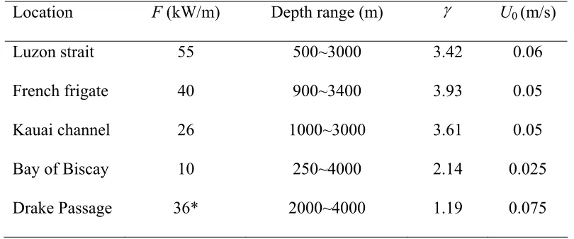
study………..36 Table 4.2 Energy fluxes and parameters at locations where strong internal waves are
LIST OF FIGURES
Figure 1.1 A sketch of internal waves
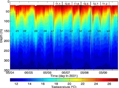
(http://whatonearth.olehnielsen.dk/oceanwaves.asp)...38 Figure 1.2 Time evolution of temperature shows the occurrence of internal solitary waves
from mooring measurement (adapted from Zhao et al.,
2006)………...…..39 Figure 1.3 Satellite images of internal solitary waves (a) from
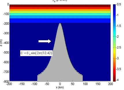
http://www.ifm.uni-hamburh.de/ers-sar/index.html and (b) adapted from Zhao et al., 2004………...40 Figure 2.1 The model configuration. Contours show the background density
field. The grey shaded area is the ridge. The model is forced by
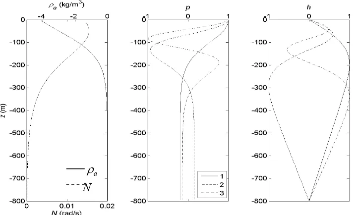
semidiurnal tide………...41 Figure 2.2 (a) Profiles of density perturbation in kg/mρa 3 and buoyancy frequency
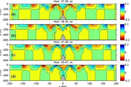
N in rad/s. The first three normal modes are shown for (b) horizontal velocity and (c) vertical velocity. Adapted from Shaw et al. (2009)…...42 Figure 3.1 Contour plots of baroclinic velocity u′ in experiment 1a with L = 15 km
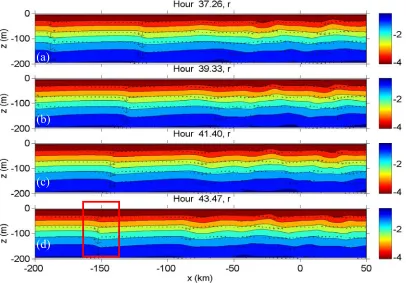
for ridge height h0 = 400 m at t = 37.26 to 43.47 hours with increments of 2 hours. The barotropic tidal flow is to the right in the two middle panels. The contour interval is 0.04 m/s………..43 Figure 3.2 Contour plots of density perturbation for experiment 1a with baroclinic
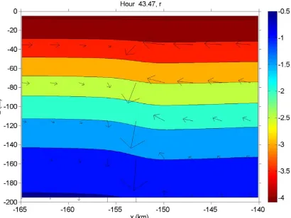
velocity vector superposed at t = 37.26 to 43.47 hours with increments of 2 hours. The contour interval is 0.5 kg/m3 ………....44 Figure 3.3 Detailed view of the density field for the red box in Figure 3.2d.
The maximum velocity is 0.14 m/s for u and 0.0061 m/s for w…………45 Figure 3.4 Contour plot of internal wave energy density at z = −5 m on the x-t
plane for experiment 1a. The contour interval is 2 W/m3………...46 Figure 3.5 Internal wave energy density for L = (a) 15, (b) 30, (c) 45, and (d) 60 km
(experiments 1a-d) with ridge height at 400 m. Energy density is the average of hourly data over three tidal cycles between t = 25.84 and
62.10 hours. The contour intervals are 2, 0.5, 0.2 and 0.2 W/m3,
Figure 3.6 Distribution of vertical energy flux at 41.40 hours in experiments (a) 1a and (b) 1d with ridge height at 400 m. The contour intervals are 0.02 and 0.002 W/m2, respectively………...48 Figure 3.7 Vertically integrated horizontal energy flux as a function of horizontal
distance for L = 15, 30, 45 and 60 km with ridge height at 400m (experiments 1a-d). The flux is averaged over three tidal cycles from
25.875 to 62.1 hours. The ridge is located at x = 0 km……...49 Figure 3.8 Distribution of time-averaged internal wave energy for U0 = (a) 0.2,
(b) 0.1, and (c) 0.05 m/s with h0 = 400 m and L = 30 km (experiments 2b, 1b, and 2a). The contour intervals are 2, 0.5 and 0.1 W/m3,
respectively………..50 Figure 3.9 Vertically integrated horizontal energy flux as a function of x for the
three experiments shown in Figure 3.8. The energy flux is normalized by
U02………...51
Figure 3.10 Distribution of internal wave energy for ridges with h0 = 400 m and L = 30 km in experiments (a) 3b, (b) 1b and (c) 3a. Time average is over the same period as in Figure 3.5. The contour intervals are 1, 0.5 and 0.1 W/m3, respectively………...52 Figure 3.11 Distribution of vertical energy flux at 41.4 hours for experiments (a) 3b
and (b) 3a. The contour intervals are 0.02 and 0.002 W/m2,
respectively……….53 Figure 3.12 Distribution of time-averaged internal wave energy for varying ridge
heights with L = 15 km. The contour intervals are 10, 2 and 0.2 W/m3, respectively……….54 Figure 3.13 Distribution of time-averaged internal wave energy for varying ridge
heights with L = 60 km. The contour intervals are 2, 0.1 and 0.05 W/m3, respectively……….55 Figure 4.1 Normalized horizontal energy flux as a function of slope parameter
Figure 4.2 Locations of the energy flux estimates in Figure
1. Introduction
1.1 Characteristics of internal waves and internal solitary waves
Internal waves propagate at the interface between the lower density water and higher density water in the ocean’s interior. Figure 1.1 is a sketch of the internal waves. In contrast
to surface waves, internal waves usually have a larger vertical displacement and a slower speed of propagation. When the amplitude of an internal wave is large, strong convergence develops at the wave front, and internal solitary waves (ISWs) forms by wave dispersion.
Figure 1.2 gives an example of the internal solitary wave observed in mooring time series in
May 2001 in the South China Sea (Zhao et al., 2006). Strong downward motion at the interface depresses the thermocline by nearly 150 m. Waves with downward motion at the front are called depression waves and are observed in the deep ocean. Differences in the arrival times for a1-a4 (labels of ISWs) are nearly 24 hours, indicating that these waves are generated by the diurnal tides. Wave fronts marked by b1-b4 (labels of ISWs) are of the origin of the semidiurnal tide. Elevation waves with strong upward motion at the front are possible in shallow waters when the upper layer is deeper than the lower layer.
the ocean are affected by ISWs, including ocean acoustic transmission (Dushaw, 2006), sediment transport (Cacchione et al., 2002; McPhee-Shaw, 2006), biological activities (Sandstrom and Elliott, 1984), and marine structure (Osborne and Burch, 1980). Most internal waves are generated by the barotropic tidal flow over varying bottom topography. Thus energy flux of internal waves plays an important role in dissipation of barotropic tidal energy in the ocean and is of concern to mixing in the ocean (e.g. Rudnick et al, 2003).
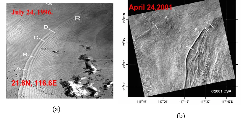
Although propagating in the ocean’s interior, ISWs are visible in the remote sensing images. Their signatures at the sea surface are produced by changes in sea surface roughness. Examples of ISWs in two satellite images in the northern South China Sea are shown in
Figure 1.3. A bright strip leading a dark strip in front of a wave group is produced by strong
convergence at the wave front of a depression wave (Figure 1.3b). In Figure 1.3a, dark
strips leading white ones represent elevation ISWs (Zhao et al., 2003; Zhao et al., 2004).
Numerical models and field observations provide detailed descriptions of the
structure of ISWs in the world’s ocean. In the Luzon Strait, internal waves are produced over steep ridges reaching the strongly stratified upper ocean (Chao et al., 2007). In mooring observations (Ramp et al., 2004; Yang et al., 2004), these internal waves evolve into
1.5~3.0 m/s, using climatological stratification in the northern South China Sea (Zhao et al 2006). Over the shallow continental shelf, polarity change from depression waves to elevation waves may take place (Zhao et al, 2006).
The ability of ISWs to propagate over long distance without changing their form is due to the balance between nonlinearity and dispersion (Osborn and Burch, 1980). Two mechanisms are involved in the generation of ISWs by strong tidal flow over varying bottom topography (Lamb, 1994; Farmer et al., 1999; Colosi et al., 2001). In the first generation mechanism, lee waves formed over shelf break by the ebb tide are released and evolve into ISWs toward the coast during the flood tide (Maxworthy, 1979; Apel et al., 1985; Lamb, 1994). In the second generation mechanism, internal waves are produced by tidal flow over topography; nonlinear steepening of internal tides forms the rank-ordered ISWs (Lee and Beardsley, 1974; Gerkema and Zimmerman, 1995; Holloway et al., 1997). Using idealized
nonhydrostatic simulation, Shaw et al. (2009) conclude that both generation mechanisms are crucial in the formation of ISWs in the northern South China Sea. Internal wave beams in the form of lee waves are produced by tidal flow over a ridge with supercritical slope. Wave beams then develop into horizontally propagating internal waves, which intensify to form tidal bores and internal solitary waves. A sharp thermocline in the upper ocean is required to trap energy in a wave guide to develop ISWs.
1.2 Energy flux of internal waves
away from the topography, and used for the local mixing at the topography. Estimating the baroclinic energy flux converted from the barotropic tides into the internal wave fields requires understanding of the generation mechanisms of internal waves.
The baroclinic energy flux F generated over a ridge by the barotropic tides depends on the topographic width L, the topographic height h0, total water depth H, amplitude of tidal current U0, forcing frequencyω, the buoyancy frequency N, and the Coriolis parameter f. Several non-dimensional parameters can be defined: topographic slope α = h0/L, relative topographic heightδ =h H0/ , slope of the internal wave beam
, the local Froude number
(
) (
)
1/22 2 / 2 2
s=⎡⎣ ω − f N −ω ⎤⎦ Fr =U0/
(
Nh0)
)
, the tidal excursion
parameterRL =U0/
(
ωL , and the relative steepnessγ α= /s(e.g., Legg et al., 2006; Garrett and Kunze, 2007; Legg et al., 2008). The ridge is classified as supercritical ifγ >1 and subcritical ifγ <1.Linear theory of energy conversion is reviewed by Garrett and Kunze (2007). The solution in an ocean of infinite depth in the limitγ 1 is given by Bell (1975). In this case, the energy flux is independent of the ridge slope (Llewellyn Smith and Young, 2002). Balmforth et al. (2002) found modest increase in energy conversion with γ in 0≤γ<1 in an infinitely deep ocean and demonstrated the development of sharp wave beams
whenγ approaches 1. The infinite-depth solution establishes a scaling factor for energy flux:
2 2
(
2 2) (
1/2 2 2)
1/20 0 0 1 /
whereρ0is a reference density.
In an ocean of finite depth, the prediction of Bell (1975) can be significantly reduced over extended topographic features (Khatiwala, 2003) or when the length scale of the
topography is larger than the horizontal wavelength of the internal tides (Llewellyn Smith and Young, 2002). The decrease is mainly due to the absence of energy flux from large-scale
components of the bottom topography (Garrett and Kunze, 2007). Khatiwala (2003) showed that the energy flux increases withγ for subcritical topography (γ <1) and becomes saturated forγ >1over truncated sinusoidal topography. St Laurent et al. (2003) found that the energy flux produced by a small knife-edge ridge (γ → ∞) is twice that atγ =1 from a
witch-of-Agnesi profile
(
)
2 ( ) m/ 1 /h x =h ⎡⎣ + x L ⎤⎦ (2)
where x is the horizontal coordinate and L is the half-width of the ridge. For a knife-edge ridge of moderate height, St Laurent et al. (2003) found that the energy flux is mostly in mode-1 waves and greatly exceeds the prediction by linear theory whenδ →1. The result is verified analytically by Llewellyn Smith and Young (2003). Llewellyn Smith and Young (2003) also suggested that the buoyancy frequency at the ridge top should be used in (1) and the ridge height is normalized in the WKB sense.
Using a nonhydrostatic numerical model, Legg and Huijts (2006) varied the
ridges. For small RL(wide ridges), mode-1 internal waves propagate away from the ridge at the forcing frequency with small energy dissipation over both small and finite-height ridges. The internal wave energy flux produced by a small ridge (large ) can be predicted by the linear theory. Increasing
r F
L
R over a small ridge leads to waves of higher vertical modes, increasing dissipation. Higher tidal harmonics in the form of wave beams emit from the topography when RL is large. Using a nonhydrostatic model, Legg and Klymak (2008) showed occurrence of overturning produced by transient hydraulic jumps in the regime of small RL and smallFr. Whenγ is large, the isopycnal displacement, normalized by , reaches a maximum, which may saturate the internal wave energy flux.
0/
U N
The equation for calculating the energy flux from a small ridge in the linear wave regime is well developed in earlier studies. For internal solitary waves, an empirical relation is needed for large topography over a range of ridge heights, topographic widths, strengths of stratification, and amplitudes of the barotropic tide. In particular, the strong stratification in the upper ocean has been shown to play an important role in the generation of internal solitary waves in the Luzon Strait (Shaw et al., 2009). Although WKB scaling has been suggested in the linear theory, it is not clear what the effect of depth-varying stratification is in the case of a steep ridge slope and large ridge height.
three different heights are studied in a nonhydrostatic numerical model. Non-dimensional relations are established for the dependence of the normalized energy flux on the slope parameterγ . The equations have many applications in the world ocean.
The outline of the thesis is as follows: Section 2 describes the model configuration and setup. Model results for three sets of experiments with different ridge heights are given in Section 3. The effects of topographic width, barotropic tidal amplitude and stratification on internal wave energy flux are studied in each set of experiments. In Section 4, a
parameterization scheme of energy flux is derived and compared with estimated fluxes from the world ocean. Section 5 and 6 are discussion and conclusions.
2. Model description and experiments
The three-dimensional nonhydrostatic numerical model of Shaw and Chao (2006) is adopted for this study. The model uses three-dimensional momentum, continuity, and density equations with Boussinesq and rigid lid approximations. The governing equations are
2 2
2
0 0
1
2 H H
D
p g A
Dt z ρ ν ρ ρ ∂ ′ + Ω × = − ∇ − + ∇ + ∂ u
k u k u u (3)
(4) 0
∇⋅ =u
2 2 2 H H D K Dt z ρ = ∇ ρ κ+ ∂ ρ
where u is the three-dimensional velocity vector (u, v, w) in the (x, y, z) coordinates, k′ isa unit vector pointing upward from the North Pole, k is the local upward unit vector,ρ is the
deviation of density from reference density ρ0(1028 kg m−3), Ω is the Earth’s rotation rate, and p is the pressure. The kinematic viscosity and diffusivity are constant, so that AH =106 m2/s, KH = 105 m2s−1,
ν
= 1×10⁻⁴ m2s−1, and κ = 0.1×10⁻⁴ m2s−1. Equation (3) includes both the horizontal and vertical components of the Coriolis acceleration. The finite difference form of the governing equations and the solution procedure are described in Shaw and Chao (2006).The numerical experiments in this study follow those in Shaw et al. (2009) but with expanded parameter ranges. The model domain is from x = −200 km on the west side to 200 km on the east and z = −800 m at the bottom to 0 m at the surface. The horizontal and vertical grid sizes are 200 m and 10 m, respectively. An initially constant field with two grid cells is used in the y direction. By applying a periodic boundary condition, the field in the y-direction remains uniform. In effect, the three dimensional model performs a
Flow over the ridge is forced by the oscillating barotropic M2 tide with flow in the x-direction given by
U U= 0sin
( )
ωt (6)where is the tidal frequency. The barotropic tide starts from U = 0 at t = 0 and flows toward x > 0 in the first half tidal cycle. In this study, U > 0 is called the ebb tide, as in the case of the Luzon Strait.
1
1/12.42 hr 1.41 10 s
ω= − = × −4 −1
The density field consists of ambient density ρa (z) and a perturbation density anomaly ρ′ (x, z, t)
ρ ρ= a
( )
z +ρ′(
x z t, ,)
. (7)The ambient density is given by
( )
1 tanh 0 2 a z z z D ρ ρ = −∆ ⎡⎢ + ⎛⎜ − ⎝ ⎠ ⎣ ⎦ ⎤ ⎞⎟⎥ (8)
where ∆ρ is the scale of density perturbation. The thermocline is centered at depth z0 (= −50 m) with thickness D (= 120m). Figure 2.1 shows the mode configuration with the
ambient density contoures.
(
g)
1/2
1/2 0 0
0 m
0
sech sech
2 a
z z z z
g
N d dz N
D D ρ ρ ρ ρ ⎛ ∆ ⎞ ⎛ − ⎞ ⎛ − = −⎡⎣ ⎤⎦ =⎜ ⎟ ⎜ ⎟= ⎜ ⎝ ⎠ ⎝
⎝ ⎠ ax D
⎞ ⎟ ⎠ N = N (9)
with a maximum buoyancy frequencyNmaxat z = z0. The stratification
in the control experiments is obtained by setting ∆ρ = 6 kg/m max 0.015rad/s 0
N = 3 and
ρ0= 1028 kg/m3. Figure 2.2 shows the modal decomposition for this stratification. Mode-1 waves associated with (9) have zero horizontal velocity and maximum vertical velocity at z = −200 m. The phase speed of the mode-1 wave is 1.52 m/s forNmax = 0, and is proportional
to Nmax in other experiments of this study. For semidiurnal tides, the buoyancy frequency is less than the tidal frequency below z = −700 m. Extending the bottom to depths below 800 m should not affect the internal wave generation significantly.
The baroclinic velocity u′ ≡
(
u v w', ', ')
is calculated by subtracting thedepth-averaged horizontal velocity from the total velocity u. The perturbation kinetic energy
density is defined by
(
2 2 20
1
.
2
K
=
ρ
u
′
+
v
′
+
w
′
)
(10)The perturbation density ρ′ is calculated by subtracting (8) from the density field. The perturbation potential energy density is
2 2 2 0 1 . 2 g P N ρ ρ ′
The internal wave energy density E is the sum of the potential energy and kinetic energy.
The internal wave energy flux is p' 'u , wherep′is the perturbation pressure. Following Nash et al. (2005), the perturbation pressure p′ is given by
p x z t′( , , )=p x z t( , , )−p x t( , ) (12)
where pis the depth-averaged hydrostatic pressure calculated from perturbation density
1 0
(
b ( , , ))
. bz
z z
p d z x z t g d
H ρ′ ′ z
=
∫
∫
′ (13)and zb is the bottom of the z-coordinate. The total wave energy flux generated over the
topography in a region [−xB, xB] is
0 0
B
b x x b x x
z z
F
=
∫
p u
′ ′
=dz
−
∫
p u
′ ′
B
dz
=− (14)
3. Model Results
Three sets of experiments at h0 = 200 m, 400 m and 600 m, respectively, were carried out in an ocean 800 m deep. Generation of the internal wave is studied in each set of
3.1 Internal wave generation
Figure 3.1 shows the distribution of baroclinic velocity u′ during the ebb phase of the
fourth tidal cycle in experiment 1a for a ridge height of 400 m. The barotropic tidal current is zero in the first panel, eastward in the two middle panels, and zero again in the bottom panel. In Figure 3.1a, a narrow wave beam, produced by the negative tidal current in the previous
tidal phase, is present at the ridge top between z = −400 m and −200 m. The baroclinic velocity u′ is negative. In the strongly stratified upper ocean, the wave beam splits into two nearly symmetric paths away from the ridge. After the tidal current reverses direction, u′ in the wave beam becomes positive. Thus, a wave beam of positive (negative) u′ over the ridge top originates at the beginning of the ebb (flood) tide with positive (negative) tidal currents (Shaw et al. 2009).
Wave reflections by the surface occurs at x = ±26 km and ±75 km. Upward
reflections at z = −200 m, the depth of zero mode-1 horizontal velocity for profile (9), can be seen at x = ±50 km. Mode-1 waves appear beyond x = ±100 km. Intensification in the wave front of negative u′ leads to a tidal bore at x = −120 km in Figure 3.1a. This bore can be
traced back to the start of the flood tide in the second tidal cycle. As time goes by, this tidal bore gradually develops into a rank-ordered internal solitary wave train with intensification on the wave fronts. At time 43.47 hour, this rank-ordered internal solitary wave reaches about x=−153 km in Figure 3.1d. Symmetrically, ISWs with positive u′ form on the east side
The distribution of density perturbation ρ′ for experiment 1a reveals further insight into the wave generation (Figure 3.2). Over the ridge, the density surfaces are depressed
downward. The depression signal propagates away from the ridge in the form of internal waves. With sufficient tidal forcing amplitude, the front face of the depression can steepen and an internal solitary wave train gradually developes (Figure 3.2d red box).
Figure 3.3 shows the detailed view of the well developed ISW train at 43.47 hour
(red box in Figure 3.2d). The tide is at the slack water before the flood tide and the
barotropic flow field is zero at this time. A depression with amplitude 10 m is clearly seen at x=−152 km. This depression is associated with strong convergence, which produces
downward motion. The maximum downward flow is 0.006 m/s at 1 km ahead of the depression and its magnitude decreases rapidly behind the front. The maximum speed appears at the surface with magnitude of 0.14 m/s. The vertical structure is of the first baroclinic mode.
Internal wave energy density at z = −5 m for experiment 1a is shown on the x-t plane in Figure 3.4. Maxima at x = ±26 km and ±75 km indicate, respectively, the first and second
locations of wave reflection from the surface as discussed in Figure 3.1. Bands of high
data for plotting are stored hourly, insufficient to resolve the propagations of short waves in time.
3.2 Dependence of internal wave energy on the topographic width
Figure 3.5 compares the internal wave energy density for ridges of four different
widths (experiments 1a-d) but with the same height. The energy density is averaged over 3 tidal cycles starting at the third tidal cycle. The ridge top is located at the middle of the water column (h0 = 400 m). Distinct narrow internal wave beams are clearly seen over the steepest ridge slope (L = 15 km), similar to those in the u′ velocity plot in Figure 3.1. Between 200 m
and 400 m depth, wave beams are nearly vertical because of the weak stratification in the water column. In the strongly stratified upper 200 m of the water column, wave beams slant toward the horizontal direction. Symmetric wave beams appear on the two sides of the ridge. Wave reflection from the surface occurs at a location on the edge of topographic influence with maximum wave energy at the surface. Afterward, waves propagate away from the ridge in an upper ocean wave guide. Figure 3.4 shows that energy of the mode-1 waves is nearly
uniform during propagation. The decrease in energy away from the ridge is an artifact of averaging over insufficiently sampled small-scale solitary waves in hourly intervals.
Increasing the ridge half width to L = 30 km reduces the energy density and widens the wave beam (Figure 3.5b). The internal wave beams are barely visible, but the maximum
location influenced by ridge topography. The wave beam is diffused, and the location of the vertical energy maximum shifts from surface downward to 125 m depth. The internal wave energy is much reduced. A steep ridge is most efficient in producing internal waves. The different wave patterns may suggest different wave generation mechanisms over a wide ridge and a narrow ridge. The ridge slope at L = 30 km may be regarded as the critical value for transition wave structure to occur.
The vertical energy flux, wp′ at t = 41.40 hours is demonstrated in experiments with L = 15 km and 60 km (Figure 3.6). In both cases, upward energy flux occurs over the sloping
ridge face above z = −700 m, the depth where the tidal frequency equals the buoyancy frequency. However, the maximum flux over the narrow ridge is nearly 5 times greater. Above z = −200 m, the patterns are also different for these two cases. Over a narrow ridge (Figure 3.6a), wave beams of upward vertical energy flux cross over the ridge along the ray
paths shown in Figure 3.5. Downward flux occurs at |x| > 20 km in the entire water column
on both sides of the ridge beyond the topographic influence. The alternating upward and downward fluxes develop horizontal propagating internal waves. For L = 60 km (Figure 3.6b), upward energy flux is diffused horizontally on the ridge, downward energy flux occurs
Figure 3.7 shows the distribution of vertically integrated horizontal energy
flux as a function of the horizontal distance for the four ridges. The flux is
averaged over 3 tidal periods starting from the third tidal cycle as in Figure 3.5. The
horizontal energy flux increases rapidly with x over the ridge top, reaches a maximum at the location of maximum wave energy shown in Figure 3.5, and decays slightly away from the
ridge. The maximum horizontal energy flux is highest over the steepest ridge with L = 15 km. Decreasing the ridge slope decreases the horizontal energy flux. In this study, the sum of the maximum horizontal energy flux on the two sides of the ridge is used to represent the total internal wave energy flux produced over the ridge.
0 b z u p dz′ ′
∫
3.3 Dependence of internal wave energy on barotropic current amplitude
Figure 3.8 compares the internal wave energy generated by tidal currents of
amplitude 0.2, 0.1, and 0.05 m/s over a 400-m ridge with L = 30 km. The pattern of internal wave energy distribution is qualitatively similar in the three cases; only the magnitudes are different. Ripples in the case of the strongest tidal current indicate the formation of internal solitary waves. The data used in averaging are sampled every hour, inadequate to smooth out the sharp jumps near the wave front of an internal solitary wave.
Figure 3.9 demonstrates the vertically integrated horizontal energy flux normalized
by U02 for the three experiments shown in Figure 3.8. After normalization, the three curves become similar, especially in the wave generation region. Figure 3.9 validates that the
current as suggested in the linear theory (e.g. Bell, 1975; Llewellyn Smith and Young, 2002). In the range of current amplitude used in this study, strength of the barotropic tidal flow doesn’t affect internal wave generation qualitatively.
3.4 Dependence of internal wave energy on stratification
Effects of stratification on energy flux are studied in experiments 3b, 1b, and 3a with Nmax= 2N0, N0, and N0/2, respectively. In these three experiment, h0 = 400 m and L = 30
km. The distribution of internal wave energy shows qualitative differences in the three experiments. As discussed in Figure 3.5, the ridge slope in experiment 1b is near the
threshold to produce internal wave beams (Figure 3.10b). When the strength of stratification
is 2N0, wave beams clearly form in the upper ocean (Figure 3.10a). On the other hand,
wave beams are not well defined for Nmax= N0/2, and maximum internal wave energy is at the mid-depth, similar to the case with L = 60 km in Figure 3.5. Figure 3.10 indicates that
increase in the amplitude of the buoyancy frequency has a similar effect on wave energy conversion as increasing ridge slope.
The vertical energy flux at 41.40 hour in experiments 3b and 3a is shown in Figure 3.11. In weaker stratification (lower panel), energy propagation is upward below z = −200 m.
frequency at the ridge top. The area of vertical energy propagation below z = −200 m tilts horizontally, indicating a greater angle between the wave beam and the vertical axis, again consistent with linear theory. Upward energy propagation appears in the two slanting wave beams above z = −200 m over the ridge. The effect is to move the location of reflection from surface beyond x = ±30 km. The region of downward energy flux is now beyond topographic influence, and a large amount of internal wave energy propagates away from the ridge.
Figure 3.11 shows that stratification plays a crucial role in the wave generation mechanism;
the stronger the stratification, the more conducive to the formation of wave beams and the larger energy flux away from the ridge.
3.5 Effects of ridge height on internal wave energy
Experiment 1a with L = 15 km is extended to ridge heights h0 = 200 and 600 m with
the same tidal amplitude and stratification. Figure 3.12 shows that internal waves generated
in these three experiments are similar qualitatively. Above z = −200 m, wave beams form at nearly the same locations in all cases. However, the maximum energy is much reduced when the ridge height decreases. The ratio of energy from the smallest ridge to the tallest ridge is 1:7.5:30.
ridge top is1:5:24. It seems that the energy ratios in both Figures 3.12 and 3.13 are close to
the ratio of buoyancy frequency. However, a steep ridge slope may enhance the energy density over a tall ridge compared to that of a gentler slope ridge.
4. Parameterization of energy flux
In this study, experiments with parameters given in Table 3.1 are carried out for three
ridge heights h0 = 200, 400 and 600 m. From these experiments, a parameterization scheme can be formulated for the dependence of the vertically integrated horizontal energy flux on the topographic height, topographic half width, barotropic tidal current amplitude and stratification. The scheme is represented by a non-dimensional relation, which expresses the non-dimensional energy flux as a function of relative steepnessγ .
4.1 Dependence of non-dimensional energy flux on the slope parameter
The non-dimensional energy flux of internal waves produced over a ridge can be obtained from linear theory (1). It has been shown in Section 3.3 that is an appropriate
factor even for large ridges. However, the factor in (1) is not appropriate for tall ridges. Intuitively, we would expect that the energy flux should be proportional to the
depth-integrated barotropic tidal energy
2 0 U 2 0 h 2 0
HU . Furthermore, the choice of N is not clear for tall ridges in an ocean with buoyancy frequency varying greatly with depth. Earlier studies (e.g., Llewellyn Smith and Young, 2003) suggest that N at the ridge top be used. The
slope not just the top. Therefore, the remaining factor Nh0 in (1) is replaced by the integrated buoyancy frequency from the bottom to the depth of the ridge top. This integral relation is similar to WKB scaling. Since the buoyancy frequency decreases rapidly with depth, the stratification near the ridge top should dominate the integral consistent with the scaling in linear theory. Therefore, the following non-dimensional energy flux is used:
(15) 0 2 0 b b z h z F F = HU Ndz ρ + ′
∫
A non-dimensional parameter used in earlier studies is the slope parameterγ , the
ratio of the ridge slope to that of the wave beam. It is shown in Section 3.5 that raising and
lowering the ridge has little effect on the formation of wave beams (Figure 3.12). Therefore,
the maximum ridge slope near the top is appropriate for calculatingγ . For the depth profile
(2), the maximum topographic slope is located at /x L=1/ 3 . Because the buoyancy
frequency N is not constant in this study, the wave slope varies with depth. In Figure 3.5,
wave beams are nearly vertical below z = −200 m. Significant horizontal turning above 200
m depth indicates that the maximum slope of the wave beam is important, instead of the
depth-averaged slope over the entire water column. The maximum wave slope is obtained by
averaging the wave slope in the upper 200 m, which is the zero crossing point of the
first-mode horizontal velocity for stratification (9):
where zt = −200 m. The parameterγ is then calculated from the ratio of the ridge slope to s. The local Froude number is estimated by averaging N over the depths of the ridge, as in (15):
0
0 .
b
b
r z h
z
U F
N d z +
=
∫
(17)Table 4.1 summarizes the non-dimensional numbers for all experiments carried out in this
study.
Figure 4.1 shows the dependence of nondimensional horizontal energy flux F′ on the
relative steepnessγ obtained from all experiments. All points with ridge heights 400 and 600 m fall nicely on a curve (Figure 4.1, top panel), while the data points from the 200 m ridges
can be approximated by a different relation (Figure 4.1, bottom panel). The two relations can
be roughly classified using the Froude number (Table 2). The Froude number is less than 1.2 for ridge heights at 400 and 600 m, and greater than 1.2 for ridge height at 200 m. At the two higher ridges, the non-dimensional energy flux increases with increasingγ forγ <1 and
becomes saturated asγ increases further. The non-dimensional energy flux reaches a constant value when γ is greater than about 1.5. The transition occurs at1< <γ 1.5. The lower panel of Figure 4.1 shows the experiments of ridge height at 200 m. The non-dimensional energy
4.2 Energy flux from observations
Several field observations and numerical experiments on strong internal waves provide estimates of the non-dimensional parameters in the ocean. Figure 4.2 shows the
locations of these estimates: the Luzon Strait (L), the Hawaiian Ridge (H), which includes French Frigate and Kauai Channel, Bay of Biscay (B), and Drake Passage (DP). The internal wave energy flux in the Luzon Strait are obtained from the real-time simulation at Naval Research Laboratory in 2005 (S. F. Lin, 2009, personal communication). At French Frigate, the maximum internal wave energy flux is 39 kw/m from in-situ velocity profiles (Rudnick et al., 2003) and 45 kw/m from internal tide simulation (Simmons et al. 2004). An average
value of 40 kW/m is used. Energy fluxes in Kauai Channel and Drake Passage are reported by Simmons et al. (2004) from internal tide simulation. From the current meter measurement, Gerkema et al. (2004) estimated the energy flux in Bay of Biscay.
A note of caution needs to be mentioned. From a regional model of internal tide generation, Padman et al. (2006) estimated that the energy fluxes along the South Scotia Ridge in the Drake Passage are two orders of magnitude less than those in the global model of Simmons et al. (2004). Padman et al. (2006) suggested that the global model of Simmons et al. (2004) is not optimized for high latitude application and the South Scotia may not be a
The climatological temperature and salinity fields of Levitus (1998) are used to estimate the buoyancy frequency for the calculation of non-dimensional numbers. Bottom depth is obtained from the Gridded Earth Topography Data (ETOPO2) with 2-min resolution compiled by US Geological Survey (http://www.ngdc.noaa.gov/mgg/fliers/01mgg04.html). Topography is smoothed by a 2-D Savitzky-Golay filter using the least-squares polynomial smoothing technique (Ratzlaff and Johnson, 1989; Kuo et al., 1991). The topographic slope is then calculated from the smoothed topography as the first spatial derivatives with respect to x and y. The range for vertical integration of the buoyancy frequency over the ridge surface is determined from the smoothed topography.The ridge slope is the mean value in this depth range. In this paper, east-west transects are chosen except for the Drake Passage, where a north-south transect is chosen (Heywood et al. 2007). Typical barotropic tidal current amplitude is obtained from previous studies (e.g. Legg and Klymak, 2008; Heywood et al., 2007;Gerkema et al., 2004; Jan et al., 2008). At all locations, the local Froude number is much smaller than 1.
The calculated non-dimensional energy flux and relative steepness in the ocean are listed in Table 4.2 and represented by stars in Figure 4.1 (top panel). Estimates from
energy flux is similar to that with a slightly smallerγ , indicating that all these observations are in the supercritical wave regime.
5. Discussion
The time-averaged internal wave energy plots suggest that either waves of a vertical modal structure or wave beams may be generated over a ridge. After leaving the ridge, both wave structures evolve into waves of the first baroclinic mode adapted to the undisturbed topography. The largest energy flux is associated with wave beams. When wave amplitude is large, internal waves may develop into ISWs.
Formation of wave beams over the ridge is not affected by the amplitude of the barotropic tidal current or by varying ridge height. The two factors affect the energy flux only quantitatively. In this study, the internal wave energy flux is shown to be proportional to the square of the barotropic tidal current. The result is consistent with the linear internal wave theory (e.g. Bell, 1975; Llewellyn Smith and Young, 2002). Linear theory also suggests that energy of the internal wave is proportional to the buoyancy frequency at the ridge crest (e.g., Llewellyn Smith and Young, 2002). Lowering the ridge height in this study greatly reduces
ridge heights when normalized by the integrated buoyancy frequency and the square of tidal current amplitude. The quadratic dependence on ridge height as suggested in linear theory is not appropriate for tall ridges.
Topographic width plays an important role in the wave generation mechanism.
Internal wave beams are generated on narrow ridges with concentrated wave energy. Because of the slanting wave path and small ridge width, internal wave beams can escape the
topographic influence when reaching the surface. In the linear internal wave theory, the slope of the wave beam depends on stratification and is given
bys=tanθ =⎡
(
ω2− f2) (
/ N2−ω2)
1/ 2, where⎣ ⎤⎦ θ is the angle between the wave beam and the horizontal direction. A wave of small θ would likely escape topographic influence. Thus, increasing stratification has the same effect on formation of wave beams as decreasing ridge width. In linear theory, the effect of ridge width and wave slope is combined into a relative slope ratio γ (see review by Garrett and Kunze, 2007). When γ > 1, the ridge is supercritical, wave beams appear on the ridge and carry a large amount of baroclinic energy away from the ridge. When γ < 1, a modal structure appears, and energy is trapped in the generation region.
The dependence of the normalized energy flux on the ratio of the ridge slope to the slope of the wave beam is described by Figure 4.1 for the three ridge heights. The
normal mode structure; no wave beams form. In this group, the normalized energy flux increases with increasing γ in each ridge height group. The trend is consistent with the previous result that energy conversion from the barotropic tide to the internal wave is enhanced as the ridge slope approaches the critical value (Khatiwala, 2003; St Laurent et al, 2003; Llewellyn Smith and Young, 2003). At fixed γ, energy flux decreases with increasing ridge height. For example, at γ = 0.65, F′ is 0.35 for ridge height at 200 m and decreases to 0.12 and 0.06, respectively, for ridges at 400 m and 600 m (Table 2). In the numerical experiments, the horizontal topographic scale above the ocean floor for a 200-m ridge becomes close to the wavelength of the free propagating internal waves. The matching in horizontal scale may increase the conversion rate.
Over supercritical ridges with large slope parameterγ (indicated in ellipses), strong wave beams form as in previous studies (e.g. Balmforth et al., 2002; St. Laurent et al., 2003). The normalized energy flux reaches a constant value at ridge heights of 400 m and 600 m. The corresponding local Froude number is small. Khatiwala (2003) found similar saturation of energy flux for certain topographies when strong internal wave beams are produced. When the local Froude number is small, hydraulic jumps form over a supercritical ridge and limit the maximum isopycnal displacement (Legg and Klymak, 2008). This process may explain the energy saturation shown in Figure 4.1.
with γ for a small ridge. In the limit of a small knife-edge ridge (γ → ∞), the conversion rate increases by a factor of 2 when compared to a bell-shaped ridge of the same height at γ = 1 (Llewellyn Smith and Young, 2003; St Laurent et al., 2003). It is likely that the reduced surface area of the ridge above ocean floor decreases the vertical energy flux emitting from the ridge. Further study is needed.
The estimates of non-dimensional energy flux for the five locations in the ocean are relatively coarse. Many uncertainties are involved. The barotropic tidal current amplitude at each location is not fixed, but changes seasonally. In this study, typical values are chosen. The energy fluxes at these locations are also obtained from rough estimates based on
numerical model and observations. In addition, uncertainties exist in the depth ranges of the ridges at these locations. In reality, the topography is much more complicated than the ideal ridge in this study. There’s no effective way to accurately determine the bottom of the ridge. Even one hundred meter change in the depth range will result in huge difference in the non-dimensional energy flux. Therefore, with all these uncertainties, it is difficult to put an error bar in Figure 4.1. Nevertheless, estimates should give the correct order of magnitude
for energy fluxes.
6. Conclusions
Energy is converted from the barotropic to baroclinic field during the generation of internal waves by flow over bottom topography. Experiments are carried out using a
Numerical experiments are set up for ridges of three different heights to study the dependence of energy flux on topographic width, barotropic tidal current amplitude, and stratification.
The results show that two distinct wave generation mechanisms are involved, producing a normal mode structure or strong internal wave beams over the ridge. These different wave generation mechanisms are closely related to the topographic width and stratification. When the topographic width is small, representing steep ridges, the wave
generation process is associated with internal wave beams. On the contrary, over a wide ridge, waves over the ridge have a vertical normal mode structure. Strong stratification leads to strong internal wave beams. Under weak stratification, development of internal wave beam is hindered, and the wave field is dominated by a modal structure over the ridge. The effects of topographic width and stratification on wave generation mechanism can be summarized by the slope parameterγ . For subcritical ridges (γ < 1, a wide ridge or weak stratification), waves of vertical modes are produced on the ridge; little energy propagates away from the ridge. On the other hand, distinct wave beams appear over a supercritical ridge (γ > 1, a steep ridge or stronger stratification); a large amount of energy propagates away from the ridge. The amplitude of barotropic tidal current does not affect the wave generation mechanism but increases the amplitude of the internal wave proportionally.
REFERENCES
Apel, J.R., J.R. Holbrook, A.K. Liu and J.J. Tsai (1985), The Sulu Sea internal soliton experiment, Journal of Physical Oceanography, 15,1625-1651.
Alpers, W., La Violette PE (1993), Tide-generated nonlinear internal wave packets in the Strait of Gibraltar observed by the synthetic aperture radar aboard the ERS-1 satellite. Proc First ERS-1 Symposium - Space at the Service of our Environment, Cannes, 4-6/11/1992. ESA, Paris, ESA SP-359, 753-758.
Balmforth, N., G. Ierley, and W. Young (2002), Tidal conversion by subcritical topography, Journal of Physical Oceanography, 32, 2900–2914.
Bell, T. (1975), Lee waves in stratified flows with simple harmonic time dependence, Journal of Fluid Mechanics 67, 705-722.
Cacchione, D.A, L.F., Pratson, A.S., Ogston (2002), The shaping of continental slopes by internal tides. Science, 296, 724-727.
Chao, S.-Y., D.-S. Ko, R.-C. Lien, P.-T. Shaw (2007), Assessing the west ridge of Luzon Strait as an internal waves mediator, Journal of Oceanography 63, 897–911.
Colosi, J., A., R.C. Beardsley, J.F. Lynch, G. Gawarkiewicz, C.-S. Chiu, and A. Scotti (2001), Observations of nonlinear internal waves on the outer New England continental shelf during the summer shelf break primer study, Journal of Geophysical Research, 106(C5),9587-9601.
Dushaw, B.D. (2006), Mode-1 internal tides in the western North Atlantic Ocean, Deep Sea Research I, 53, 449-473.
Farmer, D.M. and L. Armi (1999), The generation and trapping of solitary waves over topography, Science, 283, 188-190.
Gerkema, T. and J. T. F. Zimmerman (1995), Generation of nonlinear internal tide and solitary waves, Journal of Physical Oceanography, 25, 1081-1094.
Gerkema, T., F.–P. Lam, and L. R.M. Maas (2004), Internal tides in the Bay of Biscay: conversion rates and seasonal effects, Deep Sea Res., Part II, 51, 2995-3008.
doi:10.1016/j.dsr2.2004.09.012.
Global Ocean Associates, (2004), An atlas of Internal solitary-like waves and their properties, 2nd edition http://www.internalwaveatlas.com/Atlas2_index.html.
Heywood, K.J., J. L. Collins, C.W. Hughes, and I. Vassie (2007), On the detectability of internal tides in Drake Passage, Deep-Sea Research I, 54, 1972-1984, doi:
10.1016/j.dsr.2007.08.002.
Holloway, P.E., E. Pelinovsky, T. Talipova and B. Barnes (1997), A nonlinear model of internal tide transformation on the Australian north west shelf, Journal of Physical Oceanography, 27, 871-891.
Jan, S., R. C. Lien, and C. H. Ting (2008), Numerical study of baroclinic tides in Luzon Strait, Journal of Oceanography, 64, 789-802.
Khatiwala, S. (2003), Generation of internal tides in an ocean of finite depth: analytical and numerical calculations, Deep-Sea Research I, 50, 3–21.
Kuo, J. E., H. Wang, and S. Pickup (1991), Multidimensional least-squares smoothing using orthogonal polynomials, Analytical Chemistry, 63, 630-635.
Lamb, K.G. (1994), Numerical experiments of internal wave generation by strong tidal flow across a finite-amplitude bank edge, Journal of Geophysical Research, 99, 843-864.
Lee, C.-Y. and R.C. Beardsley (1974), The generation of long nonlinear internal waves in a weakly stratified shear flow, Journal of Geophysical Research, 79, 453-462.
Legg, S., and K. Huijts (2006), Preliminary simulations of internal waves and mixing
Legg, S. and J. Klymak (2008), Internal hydraulic jumps and overturning generated by tidal flow over a tall steep ridge, Journal of Physical Oceanography, 38, 1949-1964, doi:
10.1175/2008JPO3777.1.
Lien, R.-C., T. Y. Tang, M. H. Chang and E. A. D’Asaro (2005), Energy of nonlinear internal waves in the South China Sea. Geophysical Research Letters, 32, L05615, doi:10.1029/2004GL022012.
Llewellyn Smith, S. and W. Young (2002), Conversion of the barotropic tide, Journal of Physical Oceanography, 32, 1554-1566.
Llewellyn Smith, S. and W. Young (2003), Tidal conversion at a very steep ridge, Journal of Fluid Mechanics, 495, 175–191.
Maxworthy, T. (1979), A note on the internal solitary waves produced by tidal flow over a three-dimensional ridge, Journal of Geophysical Research, 84, 338-346.
McPhee-Shaw, E. (2006), Boundary-interior exchange: reviewing the idea that internal-wave mixing enhances lateral dispersal near continental margins, Deep Sea Research II, 53, 42-59.
Merrifield, M. A., P. E. Holloway, and T. M. S. Johnston (2001), The generation of internal tides at the Hawaiian Ridge, Geophysical Research Letter, 28, 559– 562.
Nash, J. D., M. H., Alford, E., Kunze (2005), Estimating internal wave energy fluxes in the ocean. Journal of Atmospheric and Oceanic Technology, 22, 1551-1570.
Osborne, A.R., and T. Burch (1980), Internal solitons in the Andaman Sea, Science, 108, 451-460.
Padman, L., Howard, S. and Muench, R. (2006), Internal tide generation along the South Scotia Ridge, Deep-Sea Research II 53, 157-171.
Ramp, S. R., T. Y. Tang, T. F. Duda, J. F. Lynch, A. K. Liu, C.-S. Chiu, F. L. Bahr, H. Kim, and Y. Yang (2004), Internal solitions in the northern South China Sea. Part I: Sources and deep water propagation, IEEE Journal of Oceanic Engineering, 29, 1157-1181,
Ratzlaff, K. L. and J. T. Johnson (1989), Computation of two-dimensional polynomial least-squares convolution smoothing integers, Analytical Chemistry, 61, 1303-1305.
Rudnick, D., Boyd, T.J., Brainard, R.E., Carter, G.S., Egbert, G.D., Gregg, M.C., Holloway, P.E., Klymak, J.M., Kunze, E., Lee, C.M., Levine, M.D., Luther, D.S., Martin, J.P.,
Merrifield, M.A., Moum, J.N., Nash, J.D., Pinkel, R., Rainville, L., and Sanford, T.B.(2003), From tides to mixing along the Hawaiian Ridge, Science, 301, 355–357.
Sandstrom, H. and Elliott, J.A. (1984), Internal tide and solitions on the Scotia Shelf: A nutrient pump at work. Journal of Geophysical Research, 89, 6415-6426.
Scotti, A., R. C. Beardsley, and B. Butman (2007), Generation and propagation of nonlinear internal waves in Massachusetts Bay, Journal of Geophysical Research, 112, C10001, doi:10.1029/2007JC004313.
Shaw, P.-T., and S.-Y. Chao (2006), A nonhydrostatic primitive-equation model for studying small-scale processes: an object oriented approach, Continental Shelf Research, 26,
1416-1432. doi:10.1016/j.csr.200601.018.
Shaw, P.-T., D.-S. Ko., and S.-Y. Chao (2009), Internal solitary waves induced by flow over a ridge: With applications to the northern South China Sea, Journal of Geophysical Research, 114, C02019, doi:10.1029/2008JC005007.
Simmons, H.L., Hallberg, R.W., Arbic, B.K. (2004), Internal wave generation in a global baroclinic tide model. Deep-Sea Research II, 51, 3043–3068.
doi:10.1016/j.dsr2.2004.09.015.
St. Laurent, L., S. Stringer, C. Garrett, and D. Perrault-Joncas (2003), The generation of internal tides at abrupt topography. Deep-Sea Research I, 50,
987–1003.doi:10.1016/S0967-0637(03)00096-7.
Yang Y.-J., T. Y. Tang, M. H. Chang, A. K. Liu, M.-K. Hsu, and S. R. Ramp (2004), Solitons northeast of Tung-Sha Island during the ASIAEX pilot studies, IEEE Journal of Oceanic Engineering, 29, 1182-1199. doi:10.1109/JOE.2004.841424.
Zhao, Z., V. Klemas, Q. Zheng and X.H.Yan (2004), Remote sensing evidence for baroclinic tide origin of internal solitary waves in the northeastern South China Sea, Geophysical Research Letters, 31, L06302, doi:10.1029/2003GL019077.
Zhao, Z. and M. H. Alford (2006), Source and propagation of internal solitary waves in the northeastern South China Sea, Journal of Geophysical Research, 111, C11012,
Table 3.1. List of experiments for ridge height h0 = 400 m. Experiments with the same parameters are repeated for ridge heights 200 m and 600 m.
Experiments L (km) U0 (m/s) Nmax(rad/s)
1a 15 0.1 N0
1b 30 0.1 N0
1c 45 0.1 N0
1d 60 0.1 N0
2a 30 0.05 N0
2b 30 0.2 N0
3a 30 0.1 N0/2
3b 30 0.1 2N0
4a 15 0.1 N0/2
Table 4.1. Nondimensioanl parameters calculated from all experiments in this study.
Ridge height (h0) 600 m 400 m 200 m
experiment F′ γ Fr F′ γ Fr F′ γ Fr
1a 1.16 2.6 0.1 1.35 2.6 0.56 0.62 2.6 2.5
1b 0.81 1.3 0.1 1.01 1.3 0.56 0.81 1.3 2.5
1c 0.30 0.87 0.1 0.33 0.87 0.56 0.74 0.87 2.5
1d 0.06 0.65 0.1 0.12 0.65 0.56 0.35 0.65 2.5
2a 0.84 1.3 0.05 1.02 1.3 0.28 0.81 1.3 1.25
2b 0.74 1.3 0.2 0.96 1.3 1.11 0.80 1.3 5
3a 0.05 0.65 0.2 0.12 0.65 1.19 0.32 0.65 5
3b 1.08 1.83 0.07 1.24 1.83 0.37 0.80 1.83 2
4a 0.70 1.3 0.2 1.07 1.3 1.19 0.83 1.3 5
Table 4.2. Energy fluxes and parameters at locations where strong internal waves are observed.
Location F (kW/m) Depth range (m) γ U0(m/s)
Luzon strait 55 500~3000 3.42 0.06
French frigate 40 900~3400 3.93 0.05
Kauai channel 26 1000~3000 3.61 0.05
Bay of Biscay 10 250~4000 2.14 0.025
Drake Passage 36* 2000~4000 1.19 0.075
Internal waves
Surface waves
(a)
April 24,2001
July 24, 1996.
21.8N, 116.6E
(b) Figure 1.3. Satellite images of internal solitary waves (a) from
http://www.ifm.uni-hamburh.de/ers-sar/index.html and (b) adapted from Zhao et al., 2004.
(
)
0sin 2 12.42U U= πt
a
ρ
N
Figure 2.2. (a) Profiles of density perturbation in kg/m3 and buoyancy frequency
N in rad/s. The first three normal modes are shown for (b) horizontal velocity and (c) vertical velocity. Adapted from Shaw et al. (2009).
a
(a)
(b)
(c)
(d)
Figure 3.1. Contour plots of baroclinic velocity u′ in experiment 1a with L = 15 km for ridge height h0 = 400 m at t = 37.26 to 43.47 hours with increments of 2 hours. The
(a)
(b)
(c)
(d)
E (W/m3)
E (W/m3)
(a) L=15 km
(b) L=30 km
(c) L=45 km
(d) L=60 km
(a) L=15 km
(b) L=60 km
E (W/m3)
(a) U0=0. 2m/s
(b) U0=0.1m/s
(c) U0=0.05m/s
E (W/m3)
(a) 2N0
(b) N0
(c) N0/2
W/m2
(a) 2N0
(b) N0/2
E (W/m3)
(a) h0 = 600m
(b) h0 = 400m
(c) h0 = 200m
E (W/m3)
h0=600m
h0=400m
h0=200m
0.5 1 1.5 2 2.5 3 3.5 4 0 0.5 1 1.5 H H L B DP γ F′ 400m 600m obs
0.5 1 1.5 2 2.5 3 3.5 4
0.2 0.4 0.6 0.8 1 γ F′ 200m (b) (a)
Figure 4.1. Normalized horizontal energy flux as a function of slope parameter for ridge heights (a) at 400 and 600m (top panel) and (b) at 200m (lower panel). In the top panel, * represents estimates in the ocean at Drake Passage (DP), Bay of Biscay (B), and Luzon Strait (L). The Hawaiian Ridge data (H) are at French Frigate and Kauai Channel. The three
B
H L
DP