DOI: 10.1534/genetics.108.089912
Identity-by-Descent Estimation and Mapping of Qualitative Traits in
Large, Complex Pedigrees
Mark Abney
1Department of Human Genetics, University of Chicago, Chicago, Illinois 60637
Manuscript received April 4, 2008 Accepted for publication May 2, 2008
ABSTRACT
Computing identity-by-descent sharing between individuals connected through a large, complex pedigree is a computationally demanding task that often cannot be done using exact methods. What I present here is a rapid computational method for estimating, in large complex pedigrees, the probability that pairs of alleles are IBD given the single-point genotype data at that marker for all individuals. The method can be used on pedigrees of essentially arbitrary size and complexity without the need to divide the individuals into separate subpedigrees. I apply the method to do qualitative trait linkage mapping using the nonparametric sharing statisticSpairs. The validity of the method is demonstrated via simulation
studies on a 13-generation 3028-person pedigree with 700 genotyped individuals. An analysis of an asthma data set of individuals in this pedigree finds four loci withP-values,103that were not detected in prior
analyses. The mapping method is fast and can complete analyses of150 affected individuals within this pedigree for thousands of markers in a matter of hours.
C
OMPUTATION of identical-by-descent (IBD) allelesharing between related individuals is a necessary ingredient in many methods for linkage mapping of complex traits. Typically, IBD allele sharing is used either directly to assess whether affected individuals are sharing more at a locus than expected under the null hypothesis or as a component in the covariance matrix in a variance component model. A number of
algo-rithms for computing IBD exactly exist (e.g., Elston
and Stewart 1971; Lander and Green 1987;
Kruglyak et al. 1996; Fishelson and Geiger 2002); however, these methods become computationally in-feasible when pedigrees are very large and complex. Under such circumstances approximate methods be-come necessary, whether Markov chain Monte Carlo (Thompsonet al.1993; Sobeland Lange1996; Heath
1997) or regression based (Fulkeret al.1995; Almasy
and Blangero 1998). Even these methods, however,
have difficulty when the pedigree is very deep with many generations of individuals with no data.
In humans, very deep, and possibly complex, pedi-grees often arise in conjunction with genetic studies of isolated populations. Isolated populations are com-monly thought to have characteristics that may prove
advantageous for mapping (Wrightet al.1999; Peltonen
et al.2000; Escamilla2001; Shifmanand Darvasi2001; Serviceet al.2006), yet may require specialized statis-tical methods to both properly leverage these
advan-tages and provide a valid test for the presence of a
trait-influencing gene (Bourgain and Genin2005). Large
pedigrees also arise in other animal systems where breed-ing is carefully controlled. For example, there is interest in methods that are applicable to complex pedigrees for
both livestock (Thallmanet al.2001) and dogs (Sutter
and Ostrander2004).
What I present here is a rapid computational method for estimating, in large complex pedigrees, the proba-bility that pairs of alleles are IBD given the single-point genotype data at that marker for all individuals. Because the method is very fast, it can easily be used on geno-mewide data with many thousands of markers on hun-dreds of related individuals. It can be used directly to do linkage mapping with affected individuals using the
Spairs statistic or to compute approximate multipoint
probabilities both for alleles being IBD, using
regres-sion-based approaches (e.g., Almasy and Blangero
1998), and for alleles being homozygous by descent
(HBD) using a hidden Markov model (HMM) (Abney
et al.2002). Here, I describe this computational method and its application to qualitative trait linkage analysis.
Although computing Spairs is straightforward, in
prin-ciple, a number of challenges must be overcome in creating a practical and valid mapping method for very large, and possibly complex, pedigrees. In particular, it is common in studies involving large pedigrees to have one, or a few, pedigrees, making the asymptotic distri-bution of the test statistic, which is appropriate when there are many independent pedigrees, not necessarily applicable. Also, the allele-frequency distribution may have a major influence on the test statistic when 1Address for correspondence:Department of Human Genetics, University
of Chicago, 920 E. 58th St., Chicago, IL 60637. E-mail: [email protected]
inheritance information is obscured by missing data. Unfortunately, the relevant allele-frequency distribu-tion is that in the founders of the pedigree, which in large pedigrees may be many generations earlier than the sampled individuals. As a result, estimation of the founder allele-frequency distribution from the sampled data can result in a large bias of the conditional expected sharing statistic. The difficulties posed by not knowing the true allele-frequency distribution can be largely overcome through the use of simulations, but the capacity to do many simulations requires a compu-tationally efficient method, particularly when a large number of markers are involved. Below, I describe the theoretical basis of the IBD estimation method, the approximations used, and how it differs from earlier
methods that take a similar approach (Wanget al.1995;
Daviset al.1996). I then show its application to
single-point linkage mapping usingSpairs and how the
diffi-culties mentioned above are solved. The appendix
describes how to use the IBD estimation method to obtain multipoint estimates of HBD by modifying the
HMM of Abneyet al.(2002).
METHODS
IBD estimation
The objective is to compute the probability of two alleles being IBD given all available genotype data at that locus and the entire, unbroken pedigree. The method is based on the recursive strategy suggested by Wanget al.(1995) and Daviset al.(1996). In both of these studies the probability is computed in a manner analogous to the recurrence relation for kinship coef-ficients,fAB¼1
2fMB112fFB, whereMandFare the
mother and the father of individualA, and individualB
is not a descendant of A. The equivalent recurrence
equation when there are genotype data at the locus, as
given by Wanget al.(1995) and Daviset al.(1996), is
valid only when there are no missing genotypes and is
PrðA1[B1jGÞ ¼PrðA1)M1jGÞPrðM1[B1jGÞ
1PrðA1)M2jGÞPrðM2[B1jGÞ
1PrðA1)F1jGÞPrðF1[B1jGÞ
1PrðA1)F2jGÞPrðF2[B1jGÞ; ð1Þ
where PrðAi)MjjGÞis the probability that theith allele
fromAwas inherited from thejth allele ofA’s mother,
given the observed genotype data; andAi [ Bjmeans
alleleAiis IBD with allele Bj. This equation is applied repeatedly until the founders of the pedigree are reached and boundary conditions are used to obtain the probability. When there are no individuals with missing genotypes the method is both fast and returns exact probabilities.
Unfortunately, as recognized by both Wang et al.
(1995) and Daviset al.(1996), Equation 1 is not valid
when there are missing genotypes in the data. Although neither study formulated a version of Equation 1 that holds under missing data conditions, they each sug-gested approaches for this case. The most recent version
of SimIBD (Davis et al. 1996) uses a Monte Carlo
procedure where, for each realization, a random geno-type is assigned to each missing genogeno-type, and the recursive algorithm is applied. The final probability is the average of the probabilities computed at each Monte Carlo realization. In contrast, Wanget al.(1995) suggest two different possibilities. In the first, when the recursive algorithm encounters an individual who has a missing
genotype, the relevant inheritance probability [e.g.,
PrðA1)M1jGÞ] is computed by summing over all
possible genotypes for the missing data weighted by the probability of the genotype given the observed genotypes. To simplify the computation, one can use the probability of the genotype given only the genotypes of close relatives rather than all observed genotypes. The second possibility is to find the genotype configuration for all individuals with missing genotypes that has the highest probability and apply the recursive algorithm to that configuration. Finding the highest-probability ge-notype configuration, however, can be computationally demanding if there are many missing genotypes.
A common situation when analyzing large pedigrees is to have several generations of the pedigree completely untyped. None of the above strategies are entirely sufficient in such a situation. The problem is that there is little information in the untyped portion of the genealogy from which to infer the genotype probability distribution in those individuals. Simulating over valid genotype configurations can then be time consuming and, possibly, inaccurate. Summing over all possible genotypes, on the other hand, may be computationally impracticable.
The approach I propose relies on classifying individ-uals into two groups,AandS. AnSindividual is someone who either is genotyped or has at least one ancestor who
is genotyped, while anA individual is someone who is
not among theSgroup. Note that by this definition theS
group may contain individuals for whom no data were actually collected. I also define a set of individuals called ‘‘quasi-founders,’’ where each quasi-founder is either an
Sindividual with both parents in theA group or anA
individual with a spouse in S. A version of recurrence
Equation 1, reformulated to hold true even under
missing data, is applied to the S individuals until the
quasi-founders are reached, at which point boundary conditions are employed to determine the final proba-bility. This allows one to avoid using the recurrence equation over those generations with no genotype data, thereby speeding up the computation significantly. Furthermore, additional computational efficiency is gained by applying approximations designed specifi-cally to work well when the rate of missing genotype data
constraint on the rate of missing genotype data inSstill allows for potentially many generations of untyped indi-viduals inA.
The algorithm is described in four parts. First, I describe the general form of Equation 1 and how to use this as a recurrence relation by updating the genotype information the probabilities are conditional on. I then show how the conditional probability of two alleles being IBD given some genotype information should be expressed when the allelic type of either of those alleles is unknown. This provides a general expression that can be applied recursively to compute the IBD probability. Applying this expression requires computing transmission probabilities in the presence of missing data. I derive an equation for calculating this probability and describe the approximations made to assure computational efficiency. Finally, the recursive algorithm is completed by specifying the boundary conditions to the recurrence equations.
Recurrence rules: The following notation is used throughout the remainder of this article. Individuals are indicated with uppercase script characters (e.g.,A,B,M,
F), while the true genotype of, for instance, individualA
comprises two random variables (A1, A2), where the
allelesA1andA2may each take on one of theLpossible
allelic types at the locus, n1;. . .;nL. Note that the ordering ofA1andA2is arbitrary. Throughout, I assume
that the pattern of missing genotype data is noninfor-mative and that there is no genotyping error. Hence, observed allelic types indicate the true underlying genotype whereas the event that a genotype is missing provides no information, by itself, on the true genotype. Furthermore, the entire analysis is done conditional on
the pattern of missing data. I letGrepresent the
geno-type information, which, as I show below, will grow
during the course of the algorithm. Then, G ¼ gr
represents the information at therth stage, wheregr
is a vector with two elements for each quasi-founder and for each person inS, where the elementgr
A;1¼niif the allelic type of the first allele of individualAat therth stage is known to beni(i.e.,A1¼niat stager) or is equal to zero if
unknown. The vectorg0, then, has elements
represent-ing all directly observed genotype data or data that can be
inferred without ambiguity. The vector 1Ahas the same
length as gr with entries equal to zero at all locations
except for the two elements representing the alleles ofA. Then, for instance, 1Aqr, whereis the inner product, is
a vector with entries forAequal to the corresponding
entries ofgrand all other entries equal to zero.
To extend Equation 1 to the case when some genotypes are missing, first note that it includes condi-tional probabilities for descent events involving only one allele at a time fromA(e.g., {A1)M1}, {A2)M2},
etc.). In fact, ifA1came from the mother, for instance,
thenA2must have come from the father. A version of
Equation 1 that includes the descent events for the other allele and is true even with missing data is
PrðA1[B1jGÞ
¼PrðA1)M1;A2)F1jGÞPrðM1[B1jA1)M1;A2)F1;GÞ
1PrðA1)M1;A2)F2jGÞPrðM1[B1jA1)M1;A2)F2;GÞ
1PrðA1)M2;A2)F1jGÞPrðM2[B1jA1)M2;A2)F1;GÞ
1PrðA1)M2;A2)F2jGÞPrðM2[B1jA1)M2;A2)F2;GÞ
1PrðA1)F1;A2)M1jGÞPrðF1[B1jA1)F1;A2)M1;GÞ
1PrðA1)F1;A2)M2jGÞPrðF1[B1jA1)F1;A2)M2;GÞ
1PrðA1)F2;A2)M1jGÞPrðF2[B1jA1)F2;A2)M1;GÞ
1PrðA1)F2;A2)M2jGÞPrðF2[B1jA1)F2;A2)M2;GÞ; ð2Þ
whereG¼grfor all terms. This equation is valid as long
asBandAare not the same individual andBis not a
descendant ofA. IfAandBare the same individual
the equation becomes
PrðA1[A2jGÞ
¼PrðA1)M1;A2)F1jGÞPrðM1[F1jA1)M1;A2)F1;GÞ
1PrðA1)M1;A2)F2jGÞPrðM1[F2jA1)M1;A2)F2;GÞ
1PrðA1)M2;A2)F1jGÞPrðM2[F1jA1)M2;A2)F1;GÞ
1PrðA1)M2;A2)F2jGÞPrðM2[F2jA1)M2;A2)F2;GÞ: ð3Þ
Unlike Equation 1, Equations 2 and 3 are not strictly recurrence equations because the IBD probabilities on the right-hand side have additional descent conditions not present in the left-hand side probability. In the case of no missing genotype data, the equations may be
ap-plied recursively by noting that terms such as PrðM1[
B1jA1)M1;A2)F1;G¼grÞ¼PrðM1[B1jG¼grÞ on the
right-hand side of Equations 2 and ‘‘expanding’’ these terms using the appropriate recurrence relation. Also, the descent probabilities PrðA1)M1;A2)F1jG¼grÞ,
etc., are easily tabulated on the basis of the possible
genotype configurations ofA,M, andF. When there
are missing genotypes, it is still possible to employ a recursive method based on Equations 2 and 3 by
updating G with the genotype information provided
by the descent events (e.g.,A1)M1;A2)F1). To show
this I describe the application of the updating scheme to the first term on the right-hand side of Equation 2, but the arguments apply equally well to all terms on the right-hand side. First, focus on the conditional IBD probability PrðM1[B1jA1)M1;A2)F1;GÞ, keeping in
mind that Equation 2 holds only whenBis neitherAnor
a descendant ofA. IfAhas a known genotype but either
ForMdoes not, then the additional information from
the conditionsA1)M1andA2)F1must be included in
the probability calculation. If, for example,M andA
have known genotypes,Fdoes not, andA2¼nl, then
PrðM1[B1jA1)M1;A2)F1;G¼grÞ¼PrðM1[B1jF1¼nl;
G¼grÞ¼PrðM
1[B1jG¼gr11Þ, wheregr11is identical to
gr, but with component gr11
F;1¼nl. The subsequent ap-plications of the recurrence Equation 2 from this term must be done conditional onG¼gr11rather thanG¼gr.
Note that this implies that the computations must allow for the case of a partially known genotype, asF2is known
butF1may not be.
In general, then, the IBD probabilities Pr(A1 [
B1jG¼gr) and Pr(A1[A2jG¼gr) are conditional on
genotype information that results from the previous application of recurrence Equations 2 and 3. Even with the additional information, however, it is possible forA1
orB1to be unknown. In this case, the probabilities must
be written as a sum over the allelic types for the unknown alleles before the recurrence equations are applied. So, ifA1is unknown andgBr;1¼nk,
PrðA1[B1jG ¼grÞ
¼X
i;j
PrðA1[B1jG¼gr;A1¼ni;A2¼njÞ
PrðA1¼ni;A2¼njjG¼grÞ
¼PrðA1[B1jG¼gr;A1¼nkÞPrðA1¼nkjG¼grÞ:
ð4Þ
Note that in this equation Pr(A1[B1jG¼gr,A1¼nk)¼ Pr(A1[B1jG¼gr11). Then, to compute the probability
Pr(A1[B1jG¼gr) one applies Equation 2 to the
right-hand side of Equation 4, obtaining
PrðA1[B1jG¼grÞ ¼PrðA1¼nkjG¼grÞ
½PrðA1)M1;A2)F1jG¼gr11Þ
PrðM1[B1jA1)M1;A2)F1;G¼gr11Þ1 . . .:
ð5Þ
In general, if both A1 and B1 are unknown, the
summation would be over all possible values of both
A1andB1. Doing such a sum would require applying the
recursive algorithm to all terms in the sum, which can be computationally expensive even when there are few alleles. When the missing genotype rate is low this will
occur infrequently, and instead of summing both A1
andB1over all alleles, both alleles are left as unknown
and Equation 5 reduces to Equation 2. This strategy is, in effect, equivalent to computing the probabilities conditional only on genotype information ancestral
to A and B (and the other alleles of A and B if
known) and, in practice, generally serves as a very good approximation.
Equation 5 provides a general recurrence equation that may be applied recursively to determine the probability
thatA1andB1are IBD, as long asBandAare not the
same individual andBis not a descendant ofA. IfAand
Bare the same individual, Equation 3 may be generalized
similarly. To compute the IBD probability, it is necessary to determine the transmission probabilitiesfPrðA1)M1;
A2)F1jG¼gr11Þ;. . .gin the presence of missing data.
The derivation of these probabilities and the approxima-tions made are described in Equaapproxima-tions 6–10. Although only the probability PrðA1)M1;A2)F1jG ¼ gr11Þ is
computed here, extending this derivation to the other transmission probabilities is straightforward.
To compute this probability we must consider the case whereA1orA2may be unknown. IfgAr1;21¼0, one must
sum over possible values ofA2,
PrðA1)M1;A2)F1jG¼gr11Þ
¼X
i
PrðA1)M1;A2)F1jG¼gr11;A2¼niÞ
PrðA2¼nijG¼gr11Þ ð6aÞ
X
i
PrðA1)M1;A2)F1jG¼ ½1M11F11A;1
gr11;A
2¼niÞPrðA2¼nijG¼gr11Þ ð6bÞ
PrðA1)M1;A2)F1jG¼ ½1M11F11A;1 gr11Þ;
ð6cÞ
where Equation 6b is exact instead of approximate if the
genotypes ofMandFare known, and where Equation
6c results from approximating PrðA2¼nijG¼gr11Þ PrðA2¼nijG¼ ½1M11F11A;1 gr11Þ.
Approxima-tion (6c) allows one to compute the probability with-out performing a sum over all alleles by assuming that the sum over all allelic types is approximated by
the conditional probability with A2 unknown. Note
that when A2is known and equal to, for instance,nj,
Equation 6c becomes PrðA1)M1;A2)F1jG ¼ ½1M 1
1F11A gr11Þand is exact ifgMr11andgr
11
F are known.
Equation 6c says that we may approximate the
con-ditional probability of transmission events A1)M1,
A2)F1 given all the genotype data with the
probabil-ity given just the genotype data ofA;M, andF. In fact, as described below, these probabilities will be com-puted using the genotype data from first-degree rela-tives. In computing the conditional probability of these
transmission events I assumegr11
A ¼ ðxA1; xA2Þ, where
xA1 and xA2 are allowed to equal either the unknown
state 0 or one of the known allelic typesn1;. . .;nL. This allows us to replace 1A;1gr11 with 1Agr11 in
Equa-tion 6c.
The probability in Equation 6c may be computed using Bayes’ rule,
Pr½A1)M1;A2)F1jG¼ ð1M11F11AÞ gr11
¼ Prðg
r11
A ¼ ðxA1;xA2Þ jA1)M1;A2)F1;G¼˜gÞ
P2
i;j¼1PrðgAr11¼ ðxA1;xA2Þ jA1)Mi;A2)Fj;G¼˜gÞ1Prðgr11
A ¼ ðxA1;xA2Þ jA1)Fj;A2)Mi;G¼g˜Þ
;
ð7Þ
whereg˜¼ ð1M11FÞ gr11, the observed genotypes, at
the r 1 1 step, of M and F only. Consider the
numerator of this equation,
PrðgAr1;11¼xA1;g r11
A;2 ¼xA2jA1)M1;A2)F1;G¼g˜Þ
¼PrðgAr1;11¼xA1jg r11
A;2 ¼xA2;A1)M1;A2)F1;G¼g˜Þ
PrðgAr1;21¼xA2jA2)F1;G¼g˜Þ:
ð8Þ
DðA2;F1Þ ¼Prðgr11
A;2¼xA2jA2)F1;gFr1;11¼xF1;g
r11 F;2¼xF2;g
r11
M ¼ ðxM1;xM2ÞÞ
¼
1 xA2;xF1are known and IBS
0 xA2;xF1are known and not IBS
1 xA2is unknown
Prðgr11 F;1¼xA2jg
r11 F;2¼xF2;g
r11
M ¼ ðxM1;xM2ÞÞ xA2known;xF1unknown:
8 > > > < > > > :
ð9Þ
Although the probability Prðgr11
F;1 ¼xA2jg
r11 F;2 ¼xF2;
gr11
M ¼ ðxM1;xM2ÞÞin Equation 9 is conditional only on the known values ofgr11
F;2 andgr
11
M , I improve the missing
data approximations in Equations 6b and 6c by instead computing this probability conditional on the observed genotypes of all first-degree relatives ofF.
To complete the computation of Equation 8 one needs to determine the probability Prðgr11
A;1 ¼xA1jg
r11 A;2 ¼
xA2;A1)M1;A2)F1;G ¼g˜Þ. This probability is D(A1,
M1), but in the case where xA1 is known and xM1 is
unknown, the two conditions gr11
A;2 ¼xA2 and A2)F1 result in the conditional probability on the right-hand side of Equation 9 becoming Prðgr11
M;1 ¼xA1jg
r11 M;2 ¼xM2;
gr11
F ¼ ðxF1;xF2Þ;g
r11
F;1 ¼xA2Þ, whenxF1 ¼0 andxA26¼0. Hence, Prðgr11
A;1 ¼xA1jg
r11
A;2 ¼xA2;A1)M1;A2)F1;G ¼
˜
gÞ ¼DðA1;M1Þ, and combining this with Equations 9, 8,
and 7, Equation 6c becomes
PrðA1)M1;A2)F1jG ¼gr11Þ P2 DðA1;M1ÞDðA2;F1Þ
i;j¼1DðA1;MiÞDðA2;FjÞ1DðA1;FjÞDðA2;MiÞ
:
ð10Þ
Equation 10 provides a rapid means of computing the necessary descent probabilities, even in the presence of missing data, and may be applied to the recurrence relation of Equation 5 to find the probability of any two alleles being IBD. This is effective because the approx-imations in Equation 10 were chosen to minimize computation while maintaining accuracy under the
assumption that the fraction of individuals in S with
missing genotypes is not large. This strategy works well in practice because markers are usually included in a genetic analysis only if the rate of missing genotype data is low.
Computing Equation 9 may require knowing the
conditional genotype distribution of M if gr11
M is
unknown. Although this distribution is computed conditional on the genotypes of first-degree relatives,
it also depends on the relatedness ofMandF(which is
zero in outbred individuals). The current implementa-tion of the algorithm to compute this probability
ignores the relatedness of M and F because, when
there are a fair amount of genotype data among the first-degree relatives, this has a relatively small effect, unless
M and F are very closely related. The algorithm for
obtaining the conditional genotype distribution for an individual is to descend through the pedigree, one generation at a time, beginning with the quasi-founders, and for each person encountered who has missing
genotype data, compute the genotype-frequency distri-bution given the genotypes of the parents, the spouse, and the offspring. If the person is a quasi-founder, the computation is done conditional only on the offspring and population allele frequencies. If the person is not a quasi-founder, but one or both of the parents are untyped, the computation is done conditional on the genotype-frequency distribution already computed for that parent. If an offspring is untyped, that offspring is ignored in the computation. To propagate information from more distant relatives when close relatives are untyped, additional iterations could be done, as needed. Experience suggests, however, that when the rate of miss-ing genotypes is fairly low (,20% in the setS), a single pass through the pedigree is sufficient to obtain rea-sonably accurate estimates of the conditional genotype distributions in individuals with missing genotype data. The general form of Equation 10 is particularly useful in that it naturally provides a framework to include effects such as mutation and genotyping error. In particular, while normallyD(A1,M1) is the zero or one
indicator function whenxA1andxM1are known, this may be generalized to a nontrivial function of the observed genotypes. Selecting a particular model for mutation or genotyping error where the observed genotypes depend on the true underlying genotypes would allow one to devise a more general form for D(A1,M1) than what is
given in Equation 9.
Boundary conditions: The recursive algorithm is completed by specifying boundary conditions that are
applied to Equations 2 and 3 whenAandBare
quasi-founders. I assume below that the boundary conditions are applied at steptof the recurrence. The first rule is a general condition that applies to all sample individuals.
Boundary condition 1:For any alleleAiof individualA, Pr(Ai[AijG¼gt)¼1.
For the next two boundary conditions pi is the
frequency of allele i in the founding population. To
properly account for missing allele information I en-code a missing allele as 0 and use the conventionp0¼1.
I also define the following two functions,
d9rs ¼ 1 r ¼sorr ¼0 ors¼0
0 otherwise;
and
hðr;sÞ ¼
r s¼0 orr ¼s
s r ¼0
undefined otherwise:
8 < :
For notational convenience, label the alleles of A’s
genotype ðgt
A;1¼i;g t
A;2¼jÞ and the alleles of B’s
genotypeðgt
B;1 ¼k;g t
B;2¼lÞ, where any ofi,j,k,lmay
be unknown (i.e., there may be partial or no genotype
information on one or both individuals). The
condi-tional probabilities given the genotypes ofAandBin
presence of missing data, but approximate the condi-tional probability given all the genotype data.
Boundary condition 2: Let fA be the inbreeding
coefficient of individualA. WhenAis a quasi-founder,
PrðA1[A2jG ¼gtÞ PrðA1[A2jG¼gAt Þ
¼ phði;jÞfAd9ij
phði;jÞfA1ð1fAÞph2ði;jÞ
:
When the alleles are from two separate quasi-founders
AandB, one needs the condensed identity coefficients
( Jacquard1974) for the pair. Without loss of generality, I consider only the probability thatA1andB1are IBD.
Boundary condition 3: When A and B are quasi-founders,
PrðA1[B1jG ¼gtÞ Pr½A1[B1jG ¼ ðgAt ;gBtÞ
¼X
9
r¼1
Prði [kjG ¼ ðgAt ;gBtÞ;SrÞ
Pr½G ¼ ðg
t
A;gBtÞ jSrDr
P
sPr½G¼ ðgAt ;gBtÞ jSsDs
;
where Sr is condensed identity state r and Dr is its
unconditional probability.
Furthermore, the probabilities in the sum are
r Pr½i[kjG¼ ðgt
A;gBtÞ;Sr Pr½G¼ ðgAt;gBtÞ jSr
1 d9ik d9ijd9ikdil9d9jkd9jld9klpi9 i9¼h½hðh½i;j;kÞ
2 0 d9ijd9klpi9pk9
i9¼hði;jÞ;k9¼hðk;lÞ
3 d9ijd9ik
di99kphði9;kÞpl di99kphði9;kÞpl1di99lphði9;lÞpk
1
2ð2d9klÞðdi99kphði9;kÞpl1d9i9lphði9;lÞpkÞ
i9¼hði;jÞ
4 0 ð2dkl9Þd9ijpi9pkpl i9¼hði;jÞ
5 dkl9d9ikdk99iphðk9d;ik9Þ9pipjh1ðk9d;kiÞ99pjpjhðk9;jÞpi
1
2ð2d9ijÞðdk99iphðk9;iÞpj1d9k9jphðk9;jÞpiÞ
k9¼hðk;lÞ
6 0 ð2dij9Þd9klpk9pipj
k9¼hðk;lÞ
7 dikd9jl9phði;kÞphðj;lÞ
dikd9jl9phði;kÞphðj;lÞ1dild9jk9phði;lÞphðj;kÞ
1
2ð2d9ijÞð2d9klÞðd9ikd9jlphði;kÞphðj;lÞ 1d9ildjk9phði;lÞphðj;kÞÞ
8 dik9phði;kÞpjpl
dik9phði;kÞpjpl1dil9phði;lÞpjpk1djk9phðj;kÞpipl1djl9phðj;lÞpipk 1
4ð2d9ijÞð2d9klÞ
ðd9ikphði;kÞpjpl1d9ilphði;lÞpjpk 1djk9phðj;kÞpipl1djl9phðj;lÞpipkÞ
9 0 ð2dij9Þð2d9klÞpipjpkpl:
Frequency estimation: WhenA andB are not just quasi-founders but actual founders, the boundary
con-ditions reduce to those given in Wanget al.(1995) and
Daviset al.(1996). Both boundary conditions 2 and 3
depend on the allele frequencies in the founding
population, unless all the founders are genotyped. These frequencies may be estimated either from the founding population itself, if available, or through the genotypes of those individuals in the pedigree. With deep pedi-grees, where the founders lived many generations ago, it may be impossible to obtain accurate estimates of the allele frequencies in the founding population. Unless this population is large enough that genetic drift will have had a negligible effect, sampling from the present-day population from which the pedigree originated
might not provide accurate estimates of the founder-allele frequencies. Instead, founder-allele frequencies are often estimated from the genotyped study sample.
The current method uses the best linear unbiased estimator of allele frequencies of McPeeket al.(2004) to obtain estimates from the genotyped study sample. The estimator of the frequencypnfor allelenis given by
ˆpn¼ ð1tK11Þ1tK1yn;
where 1 is a vector with each element equal to one,Kis
a matrix with elementsKij¼2fijwithfijbeing the kin-ship coefficient between individualsiandj, andynis the
vector whoseith element equals one-half the number of
alleles of typenin individuali.
The danger of using the same population both for estimating frequencies and for computing sharing is that the sharing estimate will now be negatively biased. This is a general phenomenon when estimating IBD sharing among individuals and can be understood as follows. When related individuals share an allele iden-tical by state there is some probability that this allele is also shared IBD. The rarer this allele is in the founding population, the higher the probability is that these two copies were inherited from a common ancestral allele and are IBD. Conversely, an allele shared between individuals that was fairly common in the founders is relatively unlikely to be IBD. Because of genetic drift, the frequency of an allele in the typed individuals will vary from its frequency in the founding population, and, when IBD is estimated for individuals sharing this allele, the estimate will be either too high or too low depend-ing on whether the allele frequency has drifted down or up, respectively. Underestimating the probability will, on average, happen more often because common alleles, where underestimation most often takes place, are necessarily more frequent than rare alleles. Without some adjustment for this effect, Pr(A1[B1jG) will tend
to be below its expected value. The approach taken here is to use simulations to estimate the amount of bias when the allele frequencies are estimated. This is discussed in more detail below.
Linkage mapping
I implement a nonparametric, affecteds-only
map-ping method by using the sharing statistic Spairs. For
affected pairk(composed of individualsAandB),
Spairs;k¼
X2
i;j¼1
1Ai[Bj !
4fAB;
Spairs¼X
Npairs
k¼1 Spairs;k;
where 1Eis 1 ifEis true and 0 whenEis false andfABis
the kinship coefficient between A and B. Here, the
including whenAandBrepresent the same individual,
in which case 4fAB¼2ð11fAÞ and Spairs;k¼
2ð1a1[a2fAÞ, where fA is the inbreeding coefficient
ofA. Under the null hypothesis of no linkage, we have
EðSpairs;kÞ ¼0
and
EðSpairsÞ ¼0:
The definition ofSpairs,krelies on knowing the true, unobserved IBD state of the alleles. Instead, we use its expectation given the available genotype data at that locusG,
ˆ
Spairs;k¼EðSpairs;kjGÞ ¼
X2
i;j¼1
PrðAi[BjjGÞ
" #
4fAB;
ˆ
Spairs¼X
Npairs
i¼1 ˆ Spairs;k:
Linkage mapping may be undertaken by ascertaining a sample of affected individuals and computingSˆpairs;kfor every possible pair of individuals at a locus. Under the null hypothesis of no linkageSˆpairswill form a
distribu-tion with a mean of zero, whereas under the alternative of linkage there should be excess sharing andSˆpairswill
generally be positive. Hence, to test for linkage one would do a one-sided test of Sˆpairs and reject the null
hypothesis ifSˆpairs.t for some value oft.
Significance: A major challenge of the method is determining the proper statistical significance of the estimated sharingSˆpairsat a marker. Three problems, in
particular, must be overcome: (1) Computation of an exact likelihood-ratio statistic, as done in Kongand Cox (1997), is computationally prohibitive; (2) with only a single large pedigree, asymptotic theory for the
distri-bution of Sˆpairs might not hold and, hence, using a
normal distribution approximation, as in Kruglyak
et al.(1996), might not be valid; and (3) obtaining an empirical distribution forSˆpairsfor each marker,
condi-tional on that marker’s allele frequency, could entail analysis of 102–105simulated data setsper locus, depend-ing on the degree of evidence for linkage at the locus. (The varying number of simulations per locus results from a time-saving strategy of using a limited number of simulations to screen out potentially interesting markers for which more accurate empirical distribu-tions are then found.) This may be computationally impractical for data sets with many markers.
A potential solution is to develop a more computa-tionally efficient variation on approach (3), in which the screening step is based on an appropriate transforma-tion of the empirical distributransforma-tion from a single com-pletely informative marker. Because a comcom-pletely
informative marker allows immediate identification of which alleles are IBD, it is possible to rapidly compute the distribution ofSpairs. A first-passP-value could then
be estimated at each locus by comparing Sˆpairs at the
marker against this distribution. For markers showing strong evidence of linkage, the more accurate and time-consuming approach (3) could be used. The difficulty with this approach is twofold. First, the variance ofSpairs
is much larger than the variance of Sˆpairs. The less
informative the marker, the greater the difference in the
variances. For essentially any marker the P-value
ob-tained by comparingSˆpairsto the distribution ofSpairsis
far too conservative to be useful. Second, when allele
frequencies are estimated from the sample Sˆpairs is
negatively biased. Without some form of correction
theP-value becomes even more conservative.
With a fast enough method, simulations can be used to estimate the bias and variance at a marker and correct
the estimate of Sˆpairs. Note that the number of
simu-lations needed to correct the bias and variance at a marker would typically be much less than the number
needed to assess the empiricalP-value at the marker by
method (3). To do this, for each simulation the founders are given marker alleles according to the allele-frequency distribution estimated in the real data set. The allele frequencies for each simulated data set are computed from the same individuals who are typed in the real data set, and these frequencies are used to computeSˆs
pairsfor that simulation. The mean value over
the simulatedSˆs
pairs is used as an estimator for the bias,
ˆb¼PsSˆs
pairs=Nsim, where Nsim is the number of
simu-lations. The statistic for that marker is adjusted by this bias. Although this procedure can dramatically reduce the bias, it cannot completely eliminate it, even asNsim
becomes very large, because estimates of the bias are themselves biased. This comes about because the estimated frequencies are, in general, larger than the true frequencies (e.g., rare alleles are often lost) and simulating founder genotypes using these estimated frequencies results in the simulated estimates of S˜pairs
being slightly more biased than the actual data. The final result is a slight overcorrection. The ideal solution would be to use allele frequencies determined not from the study sample itself but from the population from which the founders originated.
The distribution problem is solved by assuming that the distributions ofSpairsandSˆpairshave the same shape,
but different variance. Normalizing bothSpairsandSˆpairs
to have a variance of one would allow one to compare
ˆ
Spairsto the distribution ofSpairs. I estimate the variance
ofSˆpairsfrom the values ofSˆpairss obtained from the
bias estimation procedure. A new statistic is defined as
˜
Spairs¼ ðSˆpairsˆbÞ=
ffiffiffiffiffiffiffiffiffiffiffiffiffiffiffiffiffiffiffiffiffi VarðSˆs
pairsÞ q
. The statisticS˜pairs can
now be compared directly against the empirical
distri-bution obtained for Spairs=
ffiffiffiffiffiffiffiffiffiffiffiffiffiffiffiffiffiffiffiffiffi VarðSpairsÞ p
to obtain an
marker now includes a single analysis of the real data
and analysis of Nsim simulated data sets with allele
frequencies and marker informativeness based on the real marker data. Note that in the case where the founder-allele frequencies are known, adjusting for the bias is unnecessary, but simulations are still needed to estimate VarðSˆs
pairsÞ. The procedure of adjusting the bias and
normalizing the variance has the benefit that nowS˜pairs
(and, hence, the approximateP-value) is directly
com-parable across all markers, regardless of markers’ allele-frequency distributions. This is unlikeSˆpairs, where the
distribution depends significantly on the informative-ness and allele frequencies of the marker.
In practice, the assumption that the shapes of the distribution forSpairs and Sˆpairs are identical does not
always hold for very large values of the statistics, whereP
-values are very small. In this case, the approximateP
-value obtained using the above method tends to be highly conservative. Estimates for very smallP-values can be obtained empirically by doing many simulations under the null hypothesis, using either the given or the estimated allele frequencies. Although many simu-lations are needed, the method is fast enough to be able to determine the empirical distribution of a marker under the null hypothesis for a small number of markers.
RESULTS
Simulations: Simulations were done to test the accuracy and validity of the proposed methods. Geno-type data for a designated set of individuals were obtained by assigning the founders of a pedigree a genotype at a single locus on the basis of given allele frequencies and allowing these alleles to ‘‘drop’’ through the pedigree according to Mendelian
inheri-tance. Only a single locus (i.e., not multiple linked
markers) was simulated. Three different types of markers were used in the simulations. The first was a single-nucleotide polymorphism (SNP) having two al-leles of equal frequency. The second marker repre-sented a microsatellite and had five equifrequent alleles. The third marker was meant to be representative of a ‘‘super marker,’’ where each allele is actually a haplotype of tightly linked SNPs. The strategy of using haplotypes as alleles of a marker provides a straightforward means of using multipoint data to increase information about the inheritance process. Hence, the marker has 21
alleles with allele frequencies given by 2 3 0.2, 0.12,
0.07, 0.06, 0.05, 15 3 0.02. This allele-frequency
distribution was chosen as being approximately repre-sentative of haplotype distributions for 90-kb segments on the basis of HAPMAP data for Caucasians.
Using both the method proposed here and an exact
computation as done by MERLIN (Abecasiset al.2002),
I checked the accuracy of the proposed method by estimating the number of alleles shared IBD for the two individuals in the pedigree shown by solid symbols in
Figure 1. For each of the three types of markers, 1000 simulations were done with the genotypes from the top two generations removed and 10% of the remaining genotypes randomly set to be missing. For the purposes of the proposed method, then, all individuals in the third generation from the top were considered quasi-founders. Both exact and approximate estimates of the number of alleles shared IBD were computed for each simulation with the results shown in Figure 2. The plots show good agreement between the approximate and the exact computations with the square root of the mean squared error being 0.024, 0.049, and 0.044 for the SNP, microsatellite, and haplotype markers, respectively.
The above methods were applied to simulated data sets in a large, complex pedigree taken from the Hutterite population. The Hutterites are an isolated religious sect that originated in the Tyrolean Alps during the 1500s and now largely reside in the northern
United States and western Canada (Mange 1964;
Hostetler 1974). The pedigree used here is an
extension of the pedigree described in Abney et al.
(2000), comprising 3028 individuals in 13 generations. To assess the efficacy of the bias-correcting and scaling procedures, simulations were done with 700 individuals’ assigned genotypes. These 700 are the same sample that is currently being genotyped using the Affymetrix 500k SNP array. From this group of 700, 148 have been diagnosed with bronchial hyperresponsiveness and were labeled as ‘‘affected.’’ Figures 3 and 4 show the histograms of SpairsandS˜pairs from 10,000 simulations
with the haplotype marker before and after the
bias-Figure1.—Pedigree used to compute the accuracy of the
correction and scaling procedure was applied. The distributions in Figure 4 are fairly well matched over much of the range of statistic values, indicating that the
scaled distribution ofSpairscan be used as a reference
distribution from which approximate P-values can be
obtained. It is also evident thatSpairshas a heavier tail at
very large values, resulting in generally conservative
estimates for very small approximateP-values.
The main utility of the bias-correction and scaling procedure is to put all markers in the study, regardless of
informativeness, on a common scale over which they may be compared. This allows one to select the best markers to follow up with an empirical analysis by choosing those with the largest S˜pairs (or, equivalently,
those with the smallest approximateP-value). Figure 5
compares the distributions ofS˜pairsfor the microsatellite
and SNP markers over 10,000 simulations. The two distributions show good agreement, suggestingS˜pairsis a
reliable measure for selecting the markers that have the largest amount of IBD sharing. In Figure 6 the
distribu-tion of S˜pairs for the haplotype marker is compared
against the distributions of the microsatellite and SNP markers. In this case, where the allele-frequency distri-butions of the markers are radically different, the distributions do not compare as well, although the microsatellite marker distribution is notably closer to the haplotype marker distribution than is the SNP marker distribution. Most genetic mapping studies, however, tend to have markers with allele-frequency distributions that are relatively similar (e.g., all SNPs, all microsatellites, or possibly a mixture of the two),
suggesting that S˜pairs will generally be an effective
measure of sharing across markers. It is worth noting that the haplotype marker allele-frequency distribution, with many alleles with small frequencies, presents the most challenging scenario when trying to estimate the bias and scale of the distributions. Inevitably, genetic drift within the sampled population results in a number of lost alleles and frequencies within the current population that may not be very representative of the
Figure2.—Approximatevs.exact estimates of the number
of alleles shared IBD for the pair of individuals in Figure 1 (solid symbols) for a (A) the SNP marker, (B) the microsatel-lite marker, and (C) the haplotype marker.
Figure3.—Histogram of the trueSpairsstatistic (top) and of
frequencies in the founding population. This results in inefficiency in the bootstrapping method used and a less accurate estimate of the bias ofS˜pairs.
To check the type-I error rate of the empiricalP-value estimates, 5000 replicates were generated for each marker type in the Hutterite pedigree. In each replicate 910 individuals in the bottom three to four generations of the pedigree were assigned genotypes and analyses were done
with 71 individuals assigned as affected, the same indi-viduals as were previously diagnosed with asthma in this
population (Ober et al. 2000). In each replicate the
empiricalP-value of the marker was estimated on the basis of 5000 simulations. Two analyses were done within each replicate, one where 10% of the genotype data was re-moved at random to emulate missing data and another with no missing genotypes in the sample individuals. Results are in Table 1 and, when there are no missing data, show good agreement with the nominal type I error.
With 10% of data missing, the empirical P-values are
slightly conservative. This results from the empirical distribution being computed under simulations with no missing data. Although this results in slightly conservative
P-values, the computation time can be significantly
re-duced when doing 10,000–100,000 simulations. Option-ally, with data sets that can be analyzed quickly, one can condition on a particular set of individuals having missing
data to obtain more accurate empiricalP-values.
Figure4.—Histogram of the trueS
pairsstatistic (top) and of
the bias-corrected statisticS˜pairsas computed from simulated
data (bottom). Both distributions have been scaled to have equal variance.
Figure5.—QQ plot of 10,000 values ofS˜pairsfor the SNP
marker (vertical axis) and the microsatellite marker (horizon-tal axis).
Figure6.—QQ plot of 10,000 values ofS˜
pairsfor the
Asthma data set:A genome screen for asthma using 563 markers, including both microsatellites and SNPs,
that was previously published (Ober et al. 2000) was
reanalyzed using the method described here. In the previous analysis, the pedigree was divided into 20 subpedigrees with all inbreeding loops trimmed. A single-point, semiparametric method was used where a likelihood was maximized over parameters representing the penetrances, disease-susceptibility allele frequency,
and recombination frequency. A likelihood-ratiox2was
obtained by comparing to a maximized likelihood where the recombination frequency was set to 0.5. Because of the size of the subpedigrees, each marker was analyzed separately. This analysis resulted in five markers withP
-values,0.001 with the smallestP-value being 0.0002.
The genome screen data were analyzed using the
methods described here and approximateP-values were
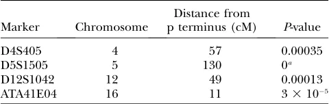
obtained for each marker. Four markers had
approxi-mateP-values,0.01 and these were selected for
follow-up with empiricalP-value estimates. EmpiricalP-values
were estimated on the basis of 100,000 simulations for each marker. Results for these four markers are shown
in Table 2. Three of the four markers had smaller P
-values than the smallestP-value of the previous analysis with two being much more significant. There was no overlap between these markers and the five markers
reported previously. ApproximateP-values for the five
markers identified earlier ranged from 0.13 to 0.65. Of the four markers identified with the new method all had
P-values.0.05 in the old analysis except for D5S1505,
which had aP-value of 0.0441. That the markers found
to have significant linkage in the two studies are different is not surprising, considering the very different methods used. The previous analysis finds markers that show some evidence for linkage under some genetic model in at least some of the subpedigrees. Although this may, it does not necessarily indicate higher than expected levels of IBD sharing among affecteds when looking at the pedigree as a whole, which is what the current method detects.
I also assessed the computation time required to do the analyses. These were accomplished on an AMD
Opteron 252 at 2.6 GHz, running Linux 2.6. The exact computation of the number of alleles shared IBD, as
done by MERLIN, for 1000 simulations, took 9.43104,
3930, and 2880 sec for the SNP, microsatellite, and haplotype markers, respectively. In contrast, the approx-imate computations took 0.4, 0.2, and 1.5 sec for the
same data sets. The empiricalP-value estimates, using
the asthma sample, took 41, 9.5, and 7 hr to estimateP
-values for 1000 markers, for the SNP, microsatellite, and haplotype markers, respectively, where the estimates were based on 5000 replicates for each marker. That is,
53106estimates of IBD sharing were computed over all
2556 pairs, averaging 0.03, 0.0068, and 0.0052 sec per
ˆ
Spairs estimate. When analyzing the real genotype data
for the asthma sample, where markers consisted of both microsatellites and SNPs of varying informativeness, each estimate ofSˆpairstook0.074 sec. This corresponds
to obtaining approximateP-values in a genome screen
of 1000 markers, with bias estimated using 50
simula-tions for each marker, in1 hr. In contrast, obtaining
empiricalP-values based on 100,000 replicates took2
hr per marker.
DISCUSSION
Linkage mapping in very large and complex pedi-grees has been a computationally daunting task. The methods proposed here are a significant step forward in making the estimation of IBD sharing feasible in pedigrees of even extremely large size and complexity. This is possible, in part, by focusing on computing pairwise IBD probabilities, rather than computing the entire distribution of IBD sharing among all individuals, and by implementing a single-point method. Also, a great deal of computational effort is saved by doing computations only on the set of quasi-founders and their descendants and using precomputed values of the identity coefficients to determine the sharing probabil-ities among the quasi-founders. This allows for efficient computation even when there are many generations of untyped individuals at the top of the pedigree. Al-though determining the identity coefficients in the quasi-founders can also be computationally challenging if the pedigree is very large, recently developed methods
TABLE 1
Empirical type I error based on 5000 replicates with different rates of missing genotypes
Type I error at a nominal type I error of Marker type Missing rate 0.05 0.01 0.005
SNP 0 0.059 0.013 0.0054
0.1 0.052 0.0102 0.0034 Microsatellite 0 0.043 0.0084 0.003
0.1 0.038 0.0076 0.0028 Haplotype 0 0.049 0.009 0.0032 0.1 0.040 0.0066 0.0018
TABLE 2
EmpiricalP-value estimates for the four markers with the smallest approximateP-values in the asthma data set
Marker Chromosome
Distance from
p terminus (cM) P-value
D4S405 4 57 0.00035
D5S1505 5 130 0a
D12S1042 12 49 0.00013
ATA41E04 16 11 33105
a
can accomplish this very efficiently (e.g., identity coef-ficients for all pairs in the genotyped sample from the
pedigree described above can be done in,1 day) (M.
Abney, unpublished data). The most significant
weak-ness of this approach is the single-point nature of the method. However, being able to do a single-point com-putation is often an integral part of a more general
mul-tipoint method. Indeed, as described in theappendix, I
have used the method described here to extend the
multipoint HBD method (Abneyet al.2002) to use the
genotype data from all individuals in the pedigree. Nevertheless, even a single-point method of estimating IBD can prove useful. In particular, as markers become more informative the amount of information gained from a multipoint method decreases. Tightly linked SNPs, for instance, can be combined into haplotypes that can be treated as alleles of a highly informative super marker. Such a super marker would require inferring haplotypes from SNPs that have not recom-bined in the pedigree. This can be a challenging task in and of itself, but a number of methods have been
proposed recently to address this problem (O’Connell
2000; Windigand Meuwissen2004; Zhanget al.2005;
Baruchet al.2006; Alberset al.2007).
A direct application of the method is linkage map-ping for qualitative traits. In this case, one computes the
˜
Spairs statistic for affected individuals and determines
significance from a simulated distribution. There are a number of challenges inherent in accomplishing this, using pedigrees such as the one described here. A major difficulty is determining the distribution of the statistic
˜
Spairs. Because studies involving large pedigrees often
are restricted to a single, or a few, pedigrees rather than many independent ones, the usual central limit theo-rem argument may not lead to an accurate approxima-tion of the null distribuapproxima-tion. Without a theoretical basis for the nature of the distribution, we must simulate to determine its characteristics under the null. Because an empirical distribution for a marker depends on the characteristics of that particular marker (e.g., founder allele frequencies, rates of missing data, etc.), one would, in principle, need to determine the null distri-bution for each marker in the study. This approach is problematic not only when there are many markers, but also for any single marker if the founder allele frequen-cies are not known. Here, I propose an alternative approach that may be used even when the number of markers is large. The distribution for a marker with perfect information is determined through simulation and scaled to have a mean of zero and a variance of one.
The scoreSˆpairsat a marker is then shifted—to remove
bias—and scaled to also have a variance of one, on the basis of a limited number of simulations. If the shape of the perfect marker distribution matches that of the real marker, then this provides a computationally efficient
means of obtaining a reference distribution for S˜pairs
and an approximateP-value. Although the approximate
P-values obtained in this manner are fairly accurate over
much of the 0–1 interval, theP-values tend to become
increasingly conservative as they approach zero.
Never-theless, being able to obtain rapid estimates of the P
-value allows one to select those ‘‘best’’ markers for which
to obtain a more accurate, empirical P-value from a
large number of simulations. Note that when allele frequencies are estimated from the data, additional error beyond the Monte Carlo uncertainty of simula-tions is introduced due to the bootstrap nature of simulating data conditional on the estimated allele frequencies. If at all possible, then, it is best to obtain population allele frequencies that are independent of the data. A further complication of the need to do
simulations to obtain a P-value is the difficulty of
including genotyping error. Although it is straightfor-ward to include genotyping error in the computation for IBD, when estimating significance, genotyping error would also have to be included in the simulations. An
accurate P-value, then, necessitates simulating from a
genotyping error model that is representative of the actual errors in the data. Because determination of this model may be difficult, at present the best strategy is to take any necessary precautions to ensure that errors in the genotype data are minimized.
Although the current method obtains P-values that
are smaller than those done in an earlier analysis with different methods, these results do not directly address the question of the relative power of the two approaches. The merits of the proposed method, however, can be evaluated in light of the findings of the Genetic Analysis Workshop 12, where the asthma data set described here was analyzed by a number of different research groups.
As summarized by Chapmanand Wijsman(2001, pp. S222–
In addition to linkage mapping for a qualitative trait, the proposed IBD estimation method is directly appli-cable to quantitative trait linkage mapping based on
var-iance components (Amos1994; Almasyand Blangero
1998). There, the covariance due to a quantitative trait locus (QTL) is modeled by the IBD sharing between all pairs of individuals in the pedigree. The method de-scribed here would allow rapid determination of the QTL covariance matrix for pedigrees that have been too large to consider as a whole. The variance component mapping strategy is, in many ways, considerably more
straightforward than the Spairs linkage mapping
ap-proach. Because the hypothesis test is not based explic-itly on the degree of sharing estimated, the problems associated with determining the proper distribution of the statistic (e.g., bias) are avoided. Although bias will still exist in the IBD estimates, if allele frequencies are estimated, the amount of bias for any particular pair will generally be small. In contrast, the bias when computing
ˆ
Spairscan be large because it is the sum over very many
pairs, each of which has a small amount of bias. Furthermore, an empirical distribution for the sharing statistic need not be constructed to determine statistical significance. The consequence is that it is not necessary to do the simulations at each marker to determine the bias and variance of the statistic.
The utility of a method that addresses a computation-ally difficult problem depends criticcomputation-ally on the time it takes to solve the problem, particularly when many ana-lyses and simulations are necessary. The above methods have been implemented in freely available software coded in C (available at http://www.genes.uchicago.edu/abney. html) that can analyze the data presented here with, as yet, unprecedented speed. The analyses accomplished here, using both simulated and real data, show that it is
possible to analyze large data sets (700 genotyped
individuals,150 affecteds) in a large pedigree (3000
individuals) on a timescale of hours for thousands of markers. As far as I am aware, there are no other avail-able methods that can perform linkage mapping with this quantity of data on such a large, unbroken pedigree in any reasonable length of time. With the methods and software tools introduced here researchers with large, complex pedigrees will be able to leverage their genetic data to a degree that was not possible before.
I thank Carole Ober for allowing me to use the Hutterite pedigree and asthma data and Don Conrad for his assistance in evaluating haplotype frequencies in the HAPMAP data. This work was supported by National Institutes of Health grant HG002899.
LITERATURE CITED
Abecasis, G. R., S. S. Cherny, W. O. Cooksonand L. R. Cardon,
2002 Merlin–rapid analysis of dense genetic maps using sparse gene flow trees. Nat. Genet.30:97–101.
Abney, M., M. S. McPeekand C. Ober, 2000 Estimation of variance
components of quantitative traits in inbred populations. Am. J. Hum. Genet.66:629–650.
Abney, M., C. Oberand M. S. McPeek, 2002 Quantitative-trait
ho-mozygosity and association mapping and empirical genomewide significance in large, complex pedigrees: fasting serum-insulin level in the Hutterites. Am. J. Hum. Genet.70:920–934. Albers, C. A., T. Heskesand H. J. Kappen, 2007 Haplotype
infer-ence in general pedigrees using the cluster variation method. Ge-netics177:1101–1116.
Almasy, L., and J. Blangero, 1998 Multipoint quantitative-trait
linkage analysis in general pedigrees. Am. J. Hum. Genet.62: 1198–1211.
Amos, C. I., 1994 Robust variance-components approach for
assess-ing genetic linkage in pedigrees. Am. J. Hum. Genet.54:535– 543.
Baruch, E., J. I. Weller, M. Cohen-Zinder, M. Ronand E. Seroussi,
2006 Efficient inference of haplotypes from genotypes on a large animal pedigree. Genetics172:1757–1765.
Baum, L. E., 1972 An inequality and associated maximization
tech-nique in statistical estimation for probabilistic functions of Markov processes. Inequalities3:1–8.
Bourgain, C., and E. Genin, 2005 Complex trait mapping in
iso-lated populations: Are specific statistical methods required? Eur. J. Hum. Genet.13:698–706.
Brocklebank, D., J. Gayanand L. R. Cardon, 2007 Novel
combi-natorial optimisation methods to partition large pedigrees for ge-netic analysis. The American Society of Human Gege-netics Annual Meeting, October 25, 2007, San Diego.
Chapman, N. H., and E. M. Wijsman, 2001 Introduction: linkage
analyses in the Hutterites. Genet. Epidemiol. 21(Suppl. 1): S222–S223.
Davis, S., M. Schroeder, L. R. Goldin and D. E. Weeks,
1996 Nonparametric simulation-based statistics for detecting linkage in general pedigrees. Am. J. Hum. Genet.58:867–880. Elston, R. C., and J. Stewart, 1971 A general model for the
ge-netic analysis of pedigree data. Hum. Hered.21:523–542. Escamilla, M. A., 2001 Population isolates: their special value for
locating genes for bipolar disorder. Bipolar Disord.3:299–317. Falchi, M., P. Forabosco, E. Mocci, C. C. Borlino, A. Picciauet al.,
2004 A genomewide search using an original pairwise sampling approach for large genealogies identifies a new locus for total and low-density lipoprotein cholesterol in two genetically differ-entiated isolates of sardinia. Am. J. Hum. Genet.75:1015–1031. Fishelson, M., and D. Geiger, 2002 Exact genetic linkage
compu-tations for general pedigrees. Bioinformatics18(Suppl. 1): S189– S198.
Fulker, D. W., S. S. Chernyand L. R. Cardon, 1995 Multipoint
in-terval mapping of quantitative trait loci, using sib pairs. Am. J. Hum. Genet.56:1224–1233.
Heath, S. C., 1997 Markov chain Monte Carlo segregation and
link-age analysis for oligogenic models. Am. J. Hum. Genet.61:748–760. Hostetler, J. A., 1974 Hutterite Society. Johns Hopkins University
Press, Baltimore.
Jacquard, A., 1974 The Genetic Structure of Populations.
Springer-Verlag, New York.
Kong, A., and N. J. Cox, 1997 Allele-sharing models: Lod scores and
accurate linkage tests. Am. J. Hum. Genet.61:1179–1188. Kruglyak, L., M. J. Daly, M. P. Reeve-Daly and E. S. Lander,
1996 Parametric and nonparametric linkage analysis: a unified multipoint approach. Am. J. Hum. Genet.58:1347–1363. Lander, E. S., and P. Green, 1987 Construction of multilocus
ge-netic linkage maps in humans. Proc. Natl. Acad. Sci. USA84: 2363–2367.
Liu, F., A. Kirichenko, T. Axenovich, C.vanDuijnand Y. Aulchenko,
2008 Anapproach for cutting large and complex pedigrees for linkage analysis. Eur. J. Hum. Genet.16:854–860.
Mange, A. P., 1964 Growth and inbreeding of a human isolate.
Hum. Biol.36:104–133.
McPeek, M. S., X. Wuand C. Ober, 2004 Best linear unbiased
allele-frequency estimation in complex pedigrees. Biometrics60:359– 367.
Ober, C., A. Tsalenko, R. Parryand N. J. Cox, 2000 A
second-generation genomewide screen for asthma-susceptibility alleles in a founder population. Am. J. Hum. Genet.67:1154–1162. O’Connell, J. R., 2000 Zero-recombinant haplotyping: applications
Peltonen, L., A. Palotieand K. Lange, 2000 Use of population
iso-lates for mapping complex traits. Nat. Rev. Genet.1:182–190. Rabiner, L. R., 1989 A tutorial on hidden Markov-models and
se-lected applications in speech recognition. Proc. IEEE77:257– 286.
Service, S., J. DeYoung, M. Karayiorgou, J. L. Roos, H. Pretorious et al., 2006 Magnitude and distribution of linkage disequilib-rium in population isolates and implications for genome-wide as-sociation studies. Nat. Genet.38:556–560.
Shifman, S., and A. Darvasi, 2001 The value of isolated
popula-tions. Nat. Genet.28:309–310.
Sobel, E., and K. Lange, 1996 Descent graphs in pedigree analysis:
applications to haplotyping, location scores, and marker-sharing statistics. Am. J. Hum. Genet.58:1323–1337.
Sutter, N. B., and E. A. Ostrander, 2004 Dog star rising: the
ca-nine genetic system. Nat. Rev. Genet.5:900–910.
Thallman, R. M., G. L. Bennett, J. W. Keeleand S. M. Kappes,
2001 Efficient computation of genotype probabilities for loci with many alleles: Ii. Iterative method for large, complex pedi-grees. J. Anim. Sci.79:34–44.
Thompson, E. A., S. Lin, A. B. Olshen and E. M. Wijsman,
1993 Monte Carlo analysis on a large pedigree. Genet. Epide-miol.10:677–682.
Wang, T., R. Fernando, S. Vanderbeek, M. Grossman and J.
Vanarendonk, 1995 Covariance between relatives for a marked
quantitative trait locus. Genet. Sel. Evol.27:251–274.
Windig, J., and T. Meuwissen, 2004 Rapid haplotype
reconstruc-tion in pedigrees with dense marker maps. J. Anim. Breed. Genet.121:26–39.
Wright, A. F., A. D. Carothersand M. Pirastu, 1999 Population
choice in mapping genes for complex diseases. Nat. Genet.23: 397–404.
Zhang, K., F. Sunand H. Zhao, 2005 Haplore: a program for
hap-lotype reconstruction in general pedigrees without recombina-tion. Bioinformatics21:90–103.
Communicating editor: R. W. Doerge
APPENDIX: MULTIPOINT HBD ESTIMATION
When the above algorithm is applied to the two alleles in a single individual, it provides an estimate of the probability of that individual being HBD conditional on the entire pedigree and all ancestral genotype data at
that locus. A previous method (Abney et al. 2002)
computed this probability given the pedigree and the multipoint genotype data of that individual, while the ancestral genotype data were ignored. Here I describe
how to extend the HMM in Abney et al. (2002) to
include ancestral genotype data.
An HMM is normally defined in the following way
(Baum1972; Rabiner1989). Let
akðiÞ ¼PrðO1;. . .;Ok;Qk¼iÞ
bkðiÞ ¼PrðOk11;. . .;OMjQk¼iÞ;
whereOkare the observed genotypes at markerk,Qkis
the true HBD state (i.e., HBD or not HBD) at markerk,
and M is the number of genotyped markers. These
variables follow the recurrence formulas
ak11ðiÞ ¼
X
j
akðjÞTjiPrðOk11jQk11¼iÞ
bkðiÞ ¼X
j
TijPrðOk11jQk11¼jÞbk11ðjÞ;
whereTijis the transition probabilities between statesi
andj. The probability of HBD at markertis
PrðQt¼HBDjO1;. . .;OMÞ ¼
atðPHBDÞbtðHBDÞ
iatðiÞbtðiÞ
:
ðA1Þ
Note that the quantity Pr(Ok11 j Qk11 ¼ i) in the
recurrence equations is the probability of all the genotype data at the marker given the HBD state of a single individual. To use the single-point algorithm that now includes ancestral genotype data, the HMM is modified so that the probabilities found in the re-currence formulas are rewritten using Bayes’ rule,
PrðOkjQk¼iÞ ¼
PrðQk¼ijOkÞPrðOkÞ PrðQk¼iÞ
:
The probability Pr(Qk¼IjOk) is computed as described
in themethods section, and Pr(Qk) is the inbreeding
coefficient. We do not need to compute the uncondi-tional probability of the observed genotype data at the
marker Pr(Ok) because it cancels out in Equation A1.