DOI: 10.1534/genetics.109.112979
Searching for Recursive Causal Structures in Multivariate
Quantitative Genetics Mixed Models
Bruno D. Valente,*
,†Guilherme J. M. Rosa,
†,§,1Gustavo de los Campos,
‡Daniel Gianola
†,‡,§and Martinho A. Silva*
*Department of Animal Sciences, Federal University of Minas Gerais, Belo Horizonte, MG 30123-970, Brazil and †Department of Dairy Science,‡Department of Animal Sciences and§Department of Biostatistics and
Medical Informatics, University of Wisconsin, Madison, Wisconsin 53706
Manuscript received December 9, 2009 Accepted for publication March 24, 2010
ABSTRACT
Biology is characterized by complex interactions between phenotypes, such as recursive and simultaneous relationships between substrates and enzymes in biochemical systems. Structural equation models (SEMs) can be used to study such relationships in multivariate analyses,e.g., with multiple traits in a quantitative genetics context. Nonetheless, the number of different recursive causal structures that can be used for fitting a SEM to multivariate data can be huge, even when only a few traits are considered. In recent applications of SEMs in mixed-model quantitative genetics settings, causal structures were preselected on the basis of prior biological knowledge alone. Therefore, the wide range of possible causal structures has not been properly explored. Alternatively, causal structure spaces can be explored using algorithms that, using data-driven evidence, can search for structures that are compatible with the joint distribution of the variables under study. However, the search cannot be performed directly on the joint distribution of the phenotypes as it is possibly confounded by genetic covariance among traits. In this article we propose to search for recursive causal structures among phenotypes using the inductive causation (IC) algorithm after adjusting the data for genetic effects. A standard multiple-trait model is fitted using Bayesian methods to obtain a posterior covariance matrix of phenotypes conditional to unobservable additive genetic effects, which is then used as input for the IC algorithm. As an illustrative example, the proposed methodology was applied to simulated data related to multiple traits measured on a set of inbred lines.
I
N biological systems, phenotypic traits may exert mutual effects that can be studied using recursive or simultaneous statistical models. For example, high yield in dairy cows increases the liability to certain diseases and, conversely, the presence of disease may affect yield adversely. Likewise, the transcriptome may be a func-tion of reproductive status in mammals and the latter may depend on other physiological variables. Knowl-edge of phenotype networks describing such interre-lationships can be used to predict behavior of complex systems, e.g., biological pathways underlying complex traits such as diseases, growth, and reproduction. Structural equation models (SEMs) (Wright 1921; Haavelmo 1943) are used to study recursive and simultaneous relationships among phenotypes in multivariate systems such as multiple-trait models in quantitative genetics. SEMs can produce an interpre-tation of relationships among traits that differs from that obtained with standard multiple-trait models(MTMs), where all relationships are represented by symmetric linear associations among random variables,
i.e., as measured by covariances. Unlike MTMs, in SEMs one trait can be treated as a predictor of another trait, providing a causal link between them.
Fitting SEMs requires defining a causal structure, which can be represented as a directed graph where each link between variables corresponds to a direct functional relationship (Pearl 2000). For k response variables, and considering all possible recursive and simultaneous relationships between pairs of traits, there arek(k1) possible structural coefficients. Even if only acyclic structures are considered, the number of possible causal structures still grows markedly with the number of traits (Shipley2002), such that the choice of a causal structure can become cumbersome as the number of traits increases.
Structural equation models for quantitative genetics settings were described by Gianola and Sorensen (2004). Many authors have used SEMs in the aforemen-tioned context by applying prior biological knowledge for defining causal structures (De los Campos et al. 2006a,b; Wuet al. 2007; Koniget al. 2008; DeMaturana et al. 2009; Wuet al. 2010). Typically, one model or a Supporting information is available online athttp://www.genetics.org/
cgi/content/full/genetics.109.112979/DC1.
1Corresponding author: Department of Dairy Science, 444 Animal Science Bldg., 1675 Observatory Dr., University of Wisconsin, Madison, WI 53706. E-mail: [email protected]
limited set of models (i.e., causal structures) is prese-lected, and members of the set are fit and compared on the basis of some model comparison criteria such as Akaike information criteria (AIC) (Akaike 1973) or Bayesian information criteria (BIC) (Schwarz 1978). However, the utility of this approach may be limited because the set of possible causal structures considered is narrow.
As an alternative, the notion ofd-separation (Pearl 1988, 2000) can be used to explore the space of causal hypotheses to arrive at a causal structure (or a class of observationally equivalent causal structures) that is capable of generating the observed pattern of condi-tional probabilistic independencies between variables. Algorithms that search for causal structures in extensive causal hypotheses spaces using genomic information were applied, for example, by Schadtet al. (2005), Li et al. (2006), Chen et al. (2007), Liu et al. (2008), Chaibub Neto et al. (2008), and Aten et al. (2008). However, such search algorithms have not been used yet for recovering causal structures in the context of mixed models applied to quantitative genetics, in which only phenotypic and pedigree information is available.
Algorithms based on d-separation tests search for causal structures that are compatible with conditional independencies observed in the data. However, in a mixed models context, genetic covariances act as con-founders because they are a source of phenotypic co-variance that is not due to recursive relationships among traits. Therefore, a search for causal structures performed directly on the observed data may lead to misleading results. This article contributes to the literature on SEMs by presenting a methodology that allows searching for recursive causal structures in the context of mixed models for genetic analysis of quantitative traits. The proposed methodology exploits features of the mixed model and uses the inductive causation (IC) algorithm (Vermaand Pearl1990; Pearl2000) coupled with Bayesian data an-alysis. This article is structured as follows:methodology provides a brief review of SEMs for quantitative genetics and describes the IC algorithm and how to implement it in the context of mixed models, such that the search can be performed after accounting for correlations induced by genetic effects. Next,example applies the proposed methodology to simulated data pertaining to five traits sampled from a recursive causal model in a hypothetical population with correlated inbred line effects. Finally, a discussionsection is provided, where the main features and challenges of the proposed methodology are highlighted.
METHODOLOGY
SEM: Following Gianola and Sorensen (2004), a SEM with a specific recursive causal structure and random additive genetic effects can be written as
yi¼Lyi1Xib1ui1ei; ð1Þ
whereyiis a (t31) vector of phenotypic records of the ith subject (e.g., an animal or plant); L is a (t 3 t) matrix with zeroes in the diagonal and with structural coefficients in the off-diagonal; Xib defines a linear
regression on exogenous covariates, in which the matrixXi contains the covariates andbis a vector of
‘‘fixed effects’’; and ui is a (t 3 1) vector of random
additive genetic effects and ei is a vector of model
residuals of the same dimension, both associated with theith subject.
The following joint distribution is assumed for ui
andei,
ui
ei
N 0
0 ;
G0 0
0 C0
;
whereG0andC0are the additive genetic and residual
covariance matrices, respectively. In model (1), the causal structure is defined by choosing which of the off-diagonal entries ofLare free parameters and which ones are set to zero.
From (1), the ‘‘reduced model’’ is represented as
yi ¼ ðItLÞ1Xib1ðItLÞ1ui1ðItLÞ1ei: ð2Þ
The conditional distribution of vector yi, given the location parameters b, ui, and L and the residual
covariance matrixC0, is given by
yijL;b;ui;C0
NðItLÞ1ðXib1uiÞ;ðItLÞ1C0ðItLÞ91
:
ð3Þ
The model fornsubjects is described by
y¼ ðL5InÞy1Xb1Zu1e; ð4Þ
and the joint distribution of vectorsuandeis
u
e N
0 0 ;
G05A 0
0 C05In
; ð5Þ
wherey,u, andeare, respectively, vectors of phenotypic records, additive genetic values, and model residuals sorted by trait and subject within trait, andXandZare incidence matrices relating effects inbandutoy. The model given by (4) may be rewritten as
Itn ðL5InÞ
½ y¼Xb1Zu1e; ð6Þ
so that the reduced model is
y¼½Itn ðL5InÞ1 Xb1½Itn ðL5InÞ1 Zu
1½Itn ðL5InÞ1e: ð7Þ
pðyjL;b;u;C0Þ
N ½Itn ðL5InÞ1ðXb1ZuÞ;
Itn ðL5InÞ
½ 1CI
tn ðL5InÞ
½ 91 ; ð8Þ
whereC¼C05In.
Recovering recursive causal structures: As stated, most quantitative genetics applications of SEMs so far have used prespecified causal structures. An alternative is to implement algorithms that search for a causal structure. This section describes an algorithm that performs such a search for the modelyi¼Lyi1ei. The
application of the algorithm in the context of a mixed model is presented in the next section.
A recursive causal structure is represented by a directed acyclic graph (DAG), which is a set of variables connected by directed edges (arrows) representing direct causal relationships. A path in the causal struc-ture is a sequence of connected variables, regardless of the direction of the arrows that connect them. Un-conditionally, paths allow flows of dependence between variables in their extremes, unless there is a collider (variable with arrows pointing at them from opposite directions, likec ina/c)b) in the path. Colliders block the flow of dependency in a path, which makesa
andbindependent in the structure above. Conditioning on a variable that is not in the extremes of the path blocks the flow of dependency if this variable is a noncollider (e.g., conditioning on c in a /c /b,
a)c)b, ora)c/bmakesaandbindependent) or allows the flow of dependency if this variable is a collider. Considering two variables a and b in a DAG, they are said to bed-separated conditionally on a subset
Sof variables if there are no paths that allow flows of dependency betweenaandb(i.e., no paths betweena
and b in a DAG such that all the colliders or its descendants are in S and no noncolliders are in S). Under some assumptions (which are discussed later),d -separations in the causal structure are reflected as conditional independencies in the joint probability distribution of the data. This can be explored to recover a causal structure or a class of equivalent causal struc-tures (causal strucstruc-tures that result in joint probability distributions with the same conditional independence relationships) from the joint distribution of the data (Pearl2000; Spirteset al. 2000).
The IC algorithm (Verma and Pearl 1990; Pearl 2000) can be used to recover an underlying DAG structure (or a class of observationally equivalent struc-tures) from observed associations between traits. The search is based on queries about conditional indepen-dencies between variables and on the assumption that such independencies reflect d-separations in the un-derlying DAG. The input of the algorithm is a correla-tion matrix between observable variables, from which marginal and conditional dependencies can be evalu-ated. The output is a partially oriented graph
represent-ing a class of equivalent causal structures, which generally results in an important constraint on the initial causal hypothesis space that could be used to fit the SEM. Partially oriented graphs are graphs with directed and undirected edges. The latter represent symmetric direct relationships between pairs of var-iables, since they do not specify direction of causal relationship.
Considering a set V of random variables, the IC algorithm can be described by the following steps:
1. For each pair of variablesaandbinV, search for a set of variablesSabsuch thatais independent ofbgiven Sab. If a and b are dependent for every possible
conditioning set, connectaandbwith an undirected edge. This step results in an undirected graph U. Connected variables inUare called adjacent. 2. For each pair of nonadjacent variablesaandbwith a
common adjacent variablecinU(i.e.,a–c–b), search for a setSabthat containscsuch thatais independent
of b given Sab. If this set does not exist, then add
arrowheads pointing at c (a / c ) b). If this set exists, then continue.
3. In the resulting partially oriented graph, orient as many undirected edges as possible in such a way that it does not result in new colliders or in cycles.
The goal of the first step of the algorithm is to obtain a graph that specifies pairs of traits that are directly connected by an edge, but without specifying causal direction. Adjacent variables of an undirected graph are not d-separated, regardless of the conditioning set of variables. Therefore, adjacent variables are not pro-babilistically independent given any possible set of variables.
The aim of the second step is to orient edges by searching for variables in the undirected graph where the causal paths collide. Structures where a collider is directly caused by two nonadjacent variables are called unshielded colliders (Spirtes et al. 2000). In the unshielded collider a /c ) b, variablesa and bare called parents ofc, and the latter is called child ofaand
b. Nonadjacent parents of a collider variable are d -separated given at least one set of variables, but not if conditioned to any set of variables that contains the collider. The observational consequence of this is the probabilistic dependence between the nonadjacent parents conditionally on every possible set of variables that contains the common child.
incorporated into the search algorithm, further con-straining the output by either forbidding or coercing the existence of an edge or by performing additional edge orienting (Spirteset al. 2000; Shipley2002).
The search performed by the IC algorithm relies on the connection between causal graphs and the proba-bility distributions that they generate. This connection is established on the basis of the assumption that there are no hidden variables that affect more than one of the variables considered in the search (i.e., causal suffi-ciency assumption). If this assumption does not hold, the connection between d-separations and conditional independencies may be lost. Take as an example one set of observed variablesOand two variablesaandbthat are not connected by an edge in the underlying causal structure. Ifaandbhave a common hidden cause, they are expected to be conditionally dependent given every possible set of variables in O. This would result in including a misleading edge between a and b in the partially oriented graph selected by the IC algorithm.
In the SEM presented in (1), residualseiaccount for
the effects of the remaining unknown causes of the phenotypic traits considered. The assumption of causal sufficiency implies that the search should be performed on a set of variables that includes every common cause of two or more of these variables. Therefore, under this assumption, residuals in SEMs are constructed as in-dependent, which has been an assumption in recent applications of such models to quantitative genetics (De los Campos et al. 2006a; De Maturana et al. 2009; Heringstadet al. 2009).
The queries of the IC algorithm require pairs of variables to be declared as conditionally dependent or conditionally independent. The decision is based on partial correlations estimated from a sample. Therefore, the uncertainty about the partial correlations should be accounted for in the decision required. In a frequentist approach, these statistical decisions may be done by testing the null hypothesis of a vanishing partial cor-relation. In a Bayesian approach, these decisions can be made using highest posterior density intervals for the partial correlations.
Causal structure search within a mixed models context: In the formulation described in the previous section, model residuals are regarded as independent, and recursive effects are used to model (interpret) patterns of covariability between observable variables. However, in mixed models, the patterns of covariability between phenotypes may be due either to causal links between traits or to genetic reasons. In other words, correlated random genetic effects can act as confound-ers if one tries to select a causal structure on the basis of the joint distribution of the phenotypes, even if resid-uals are assumed as independent.
Take as an example the scenarios depicted in Figure 1, where there are recursive relationships among phenotypes y1, y2, and y3, with uncorrelated residuals
Figure1.—(A–D) Causal structures for three observed
(e1, e2, and e3) and correlated additive genetic effects
(u1, u2, and u3). The connection between the causal
structure among phenotypes and their joint probability distribution does not hold in a model where genetic effects are uncontrolled hidden variables. In this case,y1
and y2 are not marginally independent in Figure 1A
because of the covariance betweenu1andu2. For the
same reason, they are not independent given the phenotypey3in Figure 1, B–D.
Nonetheless, additive relationships between individu-als give a mean for ‘‘controlling’’ for this confounder. This can be done, for example, if there is pedigree or marker information on subjects. In this approach,d-separations are reflected as conditional independencies on the dis-tribution of phenotypes after taking into account the additive genetic effects (i.e., the distribution of the pheno-types conditionally on the genetic effects). In Figure 1A,y1
andy2are independent given the additive genetic effects.
In Figures 1, B–D, the same observed variables are independent given the additive genetic effects and phenotypey3. A SEM that accounts for additive genetic
effects can be written as (2), which implies that
VarðyiÞ ¼ ðItLÞ1G0ðItLÞ91
1ðItLÞ1C0ðItLÞ91:
Note that (ItL)1G0(ItL)91and (ItL)1C0(ItL)91
are the covariance matrices of additive genetic effects (G0*) and of residuals (R0*) obtained from a standard multiple-trait mixed model that accounts for covariance between genetic effects and residuals from different traits, but not for causal relationships between pheno-types (Gianola and Sorensen 2004; Varona et al. 2007). The covariance matrix ofyican be rewritten as
Var (yi)¼G0*1R0*, and the covariance matrix between
traits conditionally on the additive genetic effects can be represented as Var(yijui)¼(ItL)1C0(ItL)91¼R0*.
Therefore, estimates ofR0* can be used to select a causal
structure among phenotypes. This (co)variance matrix can be inferred using frequentist or Bayesian methods. In a Bayesian framework one draws samples from the posterior distribution ofR0* and these samples are used
to obtain measures of uncertainty about this matrix, while accounting for uncertainty of all other parameters included in the reduced MTM. Next, we describe how to search for a causal structure in a mixed models context, using samples from the posterior distribution ofR0* as
input to the IC algorithm:
1. Fit a MTM and draw samples from the posterior distribution ofR0*.
2. Apply the IC algorithm to the posterior samples ofR0*
to make the statistical decisions required. Specifi-cally, for each query about the statistical indepen-dence between variables a and b given a set of
variables S and, implicitly, the genetic effects, do the following:
A. Obtain the posterior distribution of residual partial correlationra,bjS. These partial
correla-tions are funccorrela-tions of R0*. Therefore their
posterior distribution can be obtained by com-puting the correlation at each sample drawn from the posterior distribution ofR0*.
B. Compute the 95% highest posterior density (HPD) interval for the posterior distribution ofra,bjS.
C. If the HPD interval contains 0, declarera,bjSas null. Otherwise, declarea andbas condition-ally dependent.
3. Fit a SEM using the selected causal structure (or one member within the class of observationally equiva-lent structures retrieved by the IC algorithm) as a ‘‘TRUE’’ causal structure.
EXAMPLE
This section illustrates concepts described previously by applying the proposed methodology to simulated data. The data generating process and the models used for inferences are described first, and results are pre-sented and discussed subsequently. The analysis was carried out using programs written in R (R D evelop-mentCoreTeam 2008), which are available from the authors upon request.
Data generating process: Observations for 1800 sub-jects were generated from a recursive model involving five traits based on the acyclic causal structure consid-ered by Shipley(1997) (Figure 2), with independent residuals. In addition, it was assumed that the observed variables were affected by a system of correlated additive genetic effects simulated for 300 inbred lines, with 6 individuals observed per line.
The SEM from which data were generated can be represented as
yi1k¼m11u1k1ei1k
yi2k¼m21l21yi1k1u2k1ei2k
yi3k¼m31l32yi2k1u3k1ei3k
yi4k¼m41l42yi2k1u4k1ei4k
yi5k ¼m51l53yi3k1l54yi4k1u5k1ei5k;
whereyijkandeijkare the phenotype and residual effects
for traitj(j¼1,. . ., 5) observed on theith individual belonging to thekth inbred line,mjis the mean value of
traitj,ujkis the additive genetic effect of inbred linekfor
traitj, andljj9is the rate of change of traitjwith respect to traitj9.
derived from full-sib individuals. Therefore, the genetic relationship matrix (A) between lines was a block dia-gonal matrix in which each block consisted of a 636 matrix where the off-diagonal entries were 0.5 (additive relationship between full sibs) and the diagonal entries were 1. Vectors of additive genetic effects and residuals were sampled from uN(0, G05A) and eN(0,
C05In), respectively.
Parameters used in the simulation were arbitrarily chosen as
G0¼
100:000 47:373 20:283 38:839 9:773 100:000 31:993 46:357 49:791
100:000 60:625 14:557 symmetric 100:000 6:490
100:000
2 6 6 6 6 6 6 4 3 7 7 7 7 7 7 5 ;
C0¼
200:000 0 0 0 0
200:000 0 0 0
200:000 0 0
symmetric 200:000 0
200:000
2 6 6 6 6 6 6 4 3 7 7 7 7 7 7 5 ; m¼ 100 110 90 180 50 2 6 6 6 6 6 6 4 3 7 7 7 7 7 7 5
; and L¼
0 0 0 0 0
0:5 0 0 0 0
0 0:35 0 0 0
0 0:5 0 0 0
0 0 0:8 0:4 0
2 6 6 6 6 6 6 4 3 7 7 7 7 7 7 5 :
Inferences: Inference was based on a SEM with independent residuals as given byC0. A fully recursive
SEM, where every entry below the main diagonal ofLis
a free parameter, was used to obtain the posterior distribution of R0*. Furthermore, a SEM was fit using
the selected causal structure. The following joint prior distribution was assumed for location and dispersion parameters of model (7),
pðL;b;u;G0;C0Þ
¼pðLÞpðbÞpðujG0ÞpðG0Þ
Yt j¼1
pðcjÞ
}Nðuj0;G05AÞIWðG0jyG;G0Þ
3 Y
t
j¼1
Inv-x2ðcjjyc;s2Þ;
where N(uj0,G05A) is a multivariate normal density
centered at0with covariance matrixG05A,IW(G0jyG,
G0) is an inverse Wishart density withy
Gd.f. and scale matrixG0,Inv-x2(c
jjyc, s2) is a scaled inverse chi-square
distribution with yc d.f. and scale s2, and cj is the
variance of model residuals for trait j. Unbounded uniform distributions were assigned to each entry ofL considered as a free parameter and tob. Finally,yG,G0
,
yc, ands2were regarded as known hyperparameters of the prior distributions.
The joint posterior distribution of all unknowns in the model is then
pðL;b;u;G0;C0jyÞ
}pðyjL;b;u;C0ÞpðujG0ÞpðG0Þ
Yt j¼1
pðcjÞ:
The resulting distribution does not have a closed form, so a Gibbs sampler algorithm (Gemanand Geman1984) was employed for drawing samples from it, using fully conditional distributions. The derivations use standard results from Bayesian linear models (e.g., Sorensenand Gianola2002; Gianolaand Sorensen2004).
A single chain of 40,000 iterations was run for each model. The initial 4000 iterations of each chain were discarded as burn-in, which was conservative relative to the 312 burn-in iterations indicated by the method of Rafteryand Lewis(1992) implemented in the R BOA package (Smith2007). The remaining 36,000 iterations were regarded as samples from the posterior distribu-tions of the parameters.
Fully recursive model:To select a causal structure to be used in a SEM, an unstructured residual covariance matrix inferred by fitting a standard multiple-trait model to the data was used to search for patterns of conditional independence that guide the selection of a class of equivalent causal structures. To estimate such a matrix, the data were analyzed using a fully recursive model, with an unstructured additive genetic covari-ance matrix and a diagonal residual covaricovari-ance matrix. This model and the standard multiple-trait model have equivalent likelihoods (Varonaet al. 2007), such that Figure 2.—Diagram of the model from which simulated
data were drawn;yj is an observed measurement on traitj, ujis the additive genetic effect contributing to traitj, andej is a model residual associated with traitj. Arcs connecting
both models produce similar residual covariance matri-ces under different parameterizations. Therefore, the posterior distribution of an unstructured residual co-variance matrix for a standard multiple-trait model can be obtained by fitting a fully recursive model and then transforming the estimated parameters in each itera-tion. The fully recursive model was reparameterized as
yi ¼ ðILfrÞ1ml1ðILfrÞ1uk1ðILfrÞ1ei
¼m*l 1u*k1e*i; with
Varðe*iÞ ¼R*0¼ ðILfrÞ1CfrðILfrÞ91; whereLfris a matrix containing structural coefficients of
a fully recursive model,R0* is an unstructured residual covariance matrix (i.e., that of a classical multiple-trait model), and Cfr is the diagonal residual covariance
matrix pertaining to the fully recursive model.
The following hyperparameter values were used for fitting the fully recursive model: sfr2¼50 and yCfr¼3 for every entry of diagonal ofCfr,yG¼7, and
G0 ¼
150 0 0 0 0
0 150 0 0 0
0 0 150 0 0
0 0 0 150 0
0 0 0 0 150
2 6 6 6 6 4 3 7 7 7 7 5:
Inferring causal structure:The posterior distribution of R0* was used to select a recursive causal structure among phenotypes, via the IC algorithm. A partial correlation was considered as null if its 95% HPD interval contained 0. The partial correlation between traits a and b, conditional on a set of traits S, is re-presented asrabjS. The partial correlations are
condi-tional not only on phenotypes inSbut also on additive genetic effects, which are omitted in the notation subsequently.
Structural equation model under the selected causal structure: On the basis of the chosen causal structure from the partially oriented graph retrieved by the IC algorithm, appropriate entries of L were treated as unknown for fitting the corresponding SEM using sim-ulated data. Hyperparameter values used for the prior distributions of the dispersion parameters were those used for fitting the fully recursive model.
Results: The posterior mean of matrixR0*, obtained
by transformingCfr, was
195:588 91:008 34:821 45:990 49:147 243:162 86:383 119:874 106:481
233:320 36:905 192:070 symmetric 269:527 131:465
411:489
2 6 6 6 6 4 3 7 7 7 7 5:
Applying the first step of the IC algorithm to samples from the posterior distribution of R0* resulted in the
undirected graph depicted in Figure 3A. Pairs of variables connected by edges had nonnull partial cor-relations regardless of the conditioning set (as illus-trated in Figure 4 for pair [y1, y2] and in supporting
information,Figure S1,Figure S2,Figure S3, andFigure S4 for the remaining pairs), where the HPD of the parameters did not contain 0. On the other hand, null partial correlations were found for the remaining pairs, as shown in Figure 5.
The second step of the IC algorithm resulted in the partially oriented graph presented in Figure 3B. The sets of three variables formed by pairs of disconnected variables with one common adjacent variable in the undirected graph retrieved from the first step werey1– y2–y3,y1–y2–y4,y3–y2–y4, y2–y3–y5, y2–y4–y5, and y3–y5–y4.
All of them were declared as noncolliders by the algorithm, except for y3–y5–y4. The algorithm directed
both edges toward y5becausey3andy4did not present
null partial correlation wheny5was in the conditioning
set of variables, as shown in Figure 6.
The third step of the IC algorithm did not change the partially oriented graph retrieved from the second step, since there was no further edge orienting to be per-formed only on the basis of the residual distribution.
The output of the IC algorithm is a partially oriented acyclic graph that represents a class of equivalent structures, each of which is capable of producing the pattern of conditional independencies resulting from
R0*. The true causal structure is an instance of the
selected class, which contains only four alternative structures (Shipley2002). However, information such Figure3.—Undirected acyclic graph (A) resulting from step
as time precedence or other sources of prior knowledge may be used for further edge orienting. Take the pair [y1,y2] as an example. The existence of an edge between
this pair is recognized by the IC algorithm, indepen-dently of any sort of prior knowledge, since the cor-relation between them is not declared as null regardless of the conditional set of remaining variables (Figure 4). However, the algorithm is not able to recognize the direction of this edge, since the pair is not part of an unshielded collider and, in the structure retrieved by the second step of the algorithm, it could be directed in either way without creating new colliders or cycles in the graph. However, if one knows, for example, that y1
precedes y2 in time, this prior knowledge is not
sufficient to impose or forbid an edge between them, but it is sufficient to orient an edge already detected by the algorithm. If, say, this information is used to point the arrowhead of this edge toward y2, all remaining
edges would be oriented as in Figure 3C. Giveny1/y2,
edgesy2–y3andy2–y4should be oriented towardy3and
y4, respectively (Shipley2002). Any other configuration
would result in colliders in y2, representing a causal
structure that is not compatible withR0*.
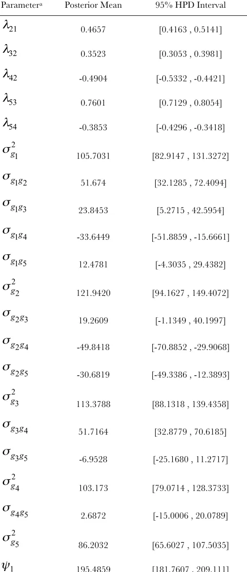
Table S1presents the posterior means and 95% HPD intervals of dispersion parameters and structural coef-ficients, obtained from a SEM fit conditionally on the causal structure chosen. Input parameter values used to simulate the data were within the aforementioned HPD intervals, with the genetic covariance between traits 2 and 5 being the exception. As additional examples, the proposed approach was used to study data simulated from two models based on different directed acyclic graphs. The results obtained from these analyses are displayed inFile S1,Figure S5, andFigure S6.
DISCUSSION
The work by Gianolaand Sorensen(2004) promp-ted interest in SEMs for analysis of quantitative traits. The authors noted the huge number of possible causal
Figure4.—Posterior
structures, even in studies with only a few traits. Wuet al. (2007) stated that prior knowledge could be used to reduce the number of causal structures under consid-eration, and this is what has been done in most of the applications of SEMs in animal breeding. However, this strategy is only as good as the preexistent theory leading to the prior knowledge (Shipley2002). Typically, prior beliefs are used to choose one structure or a small set of structures. When a set of structures is chosen, adjusted models may be compared on the basis of criteria such as AIC or BIC. However, the causal structures of the models compared are part of a small subset of all pos-sible structures, so that there may be other models that fit as well or even better than the preselected ones. One could propose an exhaustive search based on a model comparison criterion, which would require adjustment of models containing each possible causal structure. In most situations there are a huge number of possible causal structures (according to Shipley1997, there are 59,000 possible acyclic causal structures involving only five traits), which makes this approach not feasible.
Using the IC algorithm improves upon the current approach by exploring the causal structure space with-out relying only on prior causal knowledge. The algo-rithm searches for a class of equivalent acyclic causal structures compatible with the observed patterns of conditional independencies among traits. This search is not based on the aforementioned model selection criteria, although the selected structures are expected to
result in better scores for these criteria as well. This is because it returns structures that better adjust to a given pattern of conditional independencies and that are minimal; i.e., they result in SEMs with less expressive power or less flexibility when adjusting to a covariance matrix (Pearl2000). Prior beliefs may still be used to choose the more appealing structures from the structure class selected. Depending on the context, the algorithm may be modified in such a way that prior knowledge overrides the standard algorithm’s output, coercing or forbidding an edge or a direction of arrowheads to exist in the causal structure (Spirteset al. 2000).
The assumptions of the IC algorithm are not stronger than assumptions considered in recent application of SEMs in quantitative genetics. In these applications, not only covariance matrices of random variables were as-sumed to be structured (usually diagonal), but also the causal structure itself was assumed to be known. Here we impose a diagonal residual covariance matrix in the SEM, as in De losCamposet al. (2006a), DeMaturana et al. (2009), and Heringstadet al. (2009). Within this construction, a causal structure that is compatible with the joint probability distribution of the data is searched. However, the IC algorithm cannot be applied directly to the joint distribution of the phenotypes, because genetic effects may act as confounders. For the simu-lated data, applying the search algorithm on the uncon-ditional covariance matrix of the phenotypes resulted in an incorrect output for step 1: besides the undirected
Figure 5.—Posterior
edges recognized in the example described, the pairs of traits [y2,y5] and [y1,y5] were connected by edges as well.
An additional mistake was declaring the pathy3–y2–y4as
an unshielded collider (y3/y2)y4) in step 2. A main
contribution of this article was to propose a methodol-ogy of search for causal structures in the context of mixed models applied to quantitative genetics. The methodology proposed exploits the fact that it is possible to obtain the distribution of the phenotypes conditional to the genetic confounders by controlling the genetic effects. This is done by fitting a MTM, which accounts for such genetic effects.
In the example described here, all statistical decisions were correct and, consequently, alld-separations were correctly detected. The problem becomes more chal-lenging as causal relationships are weaker. After per-forming a similar simulation but with all structural coefficients reduced in absolute value by 50% (results not shown), the same undirected graph was retrieved by the first step of the algorithm. However, the second step failed to recognize the unshielded collidery3/y5)y4,
as the HPD interval ofry3y4jy5was [0.003, 0.098]. As a consequence, y5 was declared incorrectly as a
non-collider. As one would expect, statistical decisions are poorer as the posterior distribution of the partial correlations gets less sharp (e.g., smaller data sets or underidentifiability of model parameters). Less infor-mative scenarios may lead to a larger probability of incorrectly missing direct connections or adding in-correct edges, besides inin-correctly missing or adding arrowheads. After using the proposed approach on data simulated as described in the Data generating process
section, but with a single subject for each one of the 300 ‘‘inbred line effects,’’ the output was the same as that obtained when all structural coefficients were reduced in absolute value by 50%. However, the expected output was obtained when two or more subjects were simulated for each inbred line.
In these scenarios that lead to less sharp posterior distributions of the partial correlations, if statistical decisions made by the IC algorithm are based on HPD intervals of high content (which coupled with higher parameter uncertainty leads to large intervals), the algorithm looses efficiency in detecting weaker partial correlations. Since there is no preference between protecting from failure to detect nonnull partial corre-lations and declaring true null partial correcorre-lations as nonnull, it would seem sensible to decrease the prob-ability content of the HPD intervals used for decisions when the posterior distributions of partial correlations are less sharp (Shipley 2002). Nevertheless, errors in the statistical decisions do not necessarily cause mistakes in the inference. For example, if there is more than one conditioning set that d-separates two variables and some, but not all of them, mirror a vanishing partial correlation in the sample analyzed, the resulting un-directed graph would be the same, because the edges are discarded in the presence of at least one null partial correlation (Spirteset al. 2000).
Genetic effects (and their correlations) enter into both the reduced MTM and the recursive SEM. How-ever, parametric interpretations differ according to the model used. As an example, consider the additive gene-tic correlation between hypothegene-tical traitsaandb, and let a cause b. Under a recursive model, the additive genetic correlation accounts for a linear association between two unobservable variables, each directly af-fecting a specific trait. However, this would not be the sole source of genetic correlation between these traits under a model that does not account for recursiveness, because there is an indirect association between the additive genetic effect ofaand phenotypeb, mediated by phenotypea. Under the recursive model, the genetic correlation does not account for this indirect effect. On the other hand, the additive genetic correlation under a MTM accounts for all association effects, irrespective of
Figure6.—Posterior
dis-tributions and HPD inter-vals of partial correlations betweeny3andy4given ev-ery possible set of remain-ing variables containing
whether these effects are direct or otherwise in a recursive context. Because of this, the additive genetic correlation under a MTM could be different from 0 even if genetic additive effects are uncorrelated in the recursive context (Gianola and Sorensen 2004). Genetic correlations that are not mediated by causal relationships among phenotypes are confounders that do not allow a search for causal structures from phenotypic information alone. The present study pro-posed a search for causal structures in the covariance matrix ofyafter effects of such confounders are taken into account.
Controlling for additive genetic covariances restores the connection between the joint distribution of phe-notypes and causal structure. In cases where other important random effects may act as additional con-founders, such as maternal effects, R0* should be
inferred from mixed models that account for these effects as well. Furthermore, models that do not account fully for additive genetic confounder effects could lead to misleading results. For example, in a sire model, genetic effects inherited from the sire are taken into account, whereas genetic effects inherited from the dam are omitted in the model. Maternally inherited alleles, however, will be a source of covariance between pheno-types, and their effects would contribute to the residual covariance structure. Hence, the sire model will fail to remove the effect of additive genetic confounders.
The computation requirements of the proposed ap-proach increase as the set of analyzed traits gets larger. For the example presented in this article, 10 pairs of traits are analyzed in step 1 of the IC algorithm ([y1,y2],
[y1,y3], [y1,y4], [y1,y5], [y2,y3], [y2,y4], [y2,y5], [y3,y4],
[y3, y5], and [y4, y5]). For each pair, dependence was
evaluated conditionally on 8 different subsets of the remaining traits, as illustrated for [y1,y2] in Figure 4. If a
set of 4 traits is analyzed, dependencies relative to 6 pairs of variables should be assessed in the first step, each one conditionally on 4 different subsets. In a case with 6 traits, dependencies on 15 pairs of variables need to be evaluated in the first step, each one conditionally on 16 different subsets. Furthermore, increasing the number of traits or the size of the data set also increases com-putational time to fit the fully recursive model. The length of the Monte Carlo chain containing posterior samples of the residual covariance matrix also affects computational time of the proposed approach. This takes place not only because of the increased time required to sample the chain, but also because partial correlations must be calculated from each sample of the covariance matrix to obtain their posterior distribution. The described analysis was performed in a Dell Pre-cision T7400 workstation, with 16 Gb memory and CPU 64-bit dual-core Intel Xeon processors, running on Red Hat Enterprise Linux. It took 6 hr to obtain the posterior samples for the parameters of the fully re-cursive model and15 min to obtain a list of selected
partially oriented graph’s edges and unshielded col-liders from the posterior samples of the MTM residual covariance matrix.
Models that describe only the probabilistic relation-ship between traits are insufficient for predicting effects of interventions, while causal models may be used to infer how probabilities would change as a result of external interventions (Pearl 2000). The concepts described in this study apply beyond quantitative genetics. For example, the techniques for searching causal structures could be used for predicting the effect of farm management or veterinary decisions in which genetic covariances act as confounders.
The authors acknowledge comments provided by Brian Yandell and Elias Chaibub Neto on an earlier version of this manuscript. This research was funded by the Conselho Nacional de Desenvolvimento Cientı´fico e Tecnolo´gico and Coordenacxa˜o de Aperfeicxoamento de Pessoal de Nı´vel Superior, Brazil, and by the Wisconsin Agriculture Experiment Station, University of Wisconsin, Madison.
LITERATURE CITED
Akaike, H., 1973 Information theory and an extension of the maximum likelihood principle, pp. 267–291 in2nd International Symposium on Information Theory, edited by B. N. Petrovand F. Csaki. Publishing House of the Hungarian Academy of Sciences, Budapest. Aten, J. E., T. F. Fuller, A. J. Lusisand S. Horvath, 2008 Using
genetic markers to orient the edges in quantitative trait networks: the NEO software. BMC Syst. Biol.2:34.
ChaibubNeto, E., T. C. Ferrara, A. D. Attieand B. S. Yandell, 2008 Inferring causal phenotype networks from segregating populations. Genetics179:1089–1100.
Chen, L. S., F. Emmert-Streiband J. D. Storey, 2007 Harnessing naturally randomized transcription to infer regulatory relation-ships among genes. Genome Biol.8:R219.
De los Campos, G., D. Gianola, P. Boettcher and P. Moroni, 2006a A structural equation model for describing relationships between somatic cell score and milk yield in dairy goats. J. Anim. Sci.84:2934–2941.
De losCampos, G., D. Gianolaand B. Heringstad, 2006b A struc-tural equation model for describing relationships between so-matic cell score and milk yield in first-lactation dairy cows. J. Dairy Sci.89:4445–4455.
DeMaturana, E. L., X. L. Wu, D. Gianola, K. A. Weigeland G. J. M. Rosa, 2009 Exploring biological relationships between calving traits in primiparous cattle with a Bayesian recursive model. Ge-netics181:277–287.
Geman, S., and D. Geman, 1984 Stochastic relaxation, Gibbs distri-butions and Bayesian restoration of images. IEEE Trans. Patt. Anal. Mach. Intell.6:721–741.
Gianola, D., and D. Sorensen, 2004 Quantitative genetic models for describing simultaneous and recursive relationships between phenotypes. Genetics167:1407–1424.
Haavelmo, T., 1943 The statistical implications of a system of simul-taneous equations. Econometrica11:1–12.
Heringstad, B., X.-L. Wuand D. Gianola, 2009 Inferring relation-ships between health and fertility in Norwegian red cows using recursive models. J. Dairy Sci.92:1778–1784.
Konig, S., X. L. Wu, D. Gianola, B. Heringstadand H. Simianer, 2008 Exploration of relationships between claw disorders and milk yield in Holstein cows via recursive linear and threshold models. J. Dairy Sci.91:395–406.
Li, R., S. W. Tsaih, K. Shockley, I. M. Stylianou, J. Wergedalet al., 2006 Structural model analysis of multiple quantitative traits. PLoS Genet.2:e114.
Pearl, J., 1988 Probabilistic Reasoning in Intelligent Systems: Networks of Plausible Inference.Morgan Kauffman, San Mateo, CA.
Pearl, J., 2000 Causality: Models, Reasoning and Inference.Cambridge University Press, Cambridge, UK.
R DevelopmentCoreTeam, 2008 R: A Language and Environment for Statistical Computing.R Foundation for Statistical Computing, Vienna.http://www.R-project.org.
Raftery, A. E., and S. Lewis, 1992 How many iterations in the Gibbs sampler? pp. 763–773 inBayesian Statistics IV, edited by J. M. Bernardo, J. Berger, A. P. Dawid and A. F. M. Smith. Oxford University Press, Oxford.
Schadt, E. E., J. Lamb, X. Yang, J. Zhu, S. Edwardset al., 2005 An integrative genomics approach to infer causal associations be-tween gene expression and disease. Nat. Genet.37:710–717. Schwarz, G., 1978 Estimating the dimension of a model. Ann. Stat.
6:461–464.
Shipley, B., 1997 Exploratory path analysis with applications in ecology and evolution. Am. Nat.149:1113–1138.
Shipley, B., 2002 Cause and Correlation in Biology.Cambridge Univer-sity Press, Cambridge, UK/London/New York.
Smith, B. J., 2007 BOA: an R package for MCMC output conver-gence assessment and posterior inference. J. Stat. Softw.21:1–37. Sorensen, D., and D. Gianola, 2002 Likelihood, Bayesian and MCMC
Methods in Quantitative Genetics.Springer-Verlag, New York.
Spirtes, P., C. Glymourand R. Scheines, 2000 Causation, Prediction and Search, Ed. 2. MIT Press, Cambridge, MA.
Varona, L., D. Sorensenand R. Thompson, 2007 Analysis of litter size and average litter weight in pigs using a recursive model. Ge-netics177:1791–1799.
Verma, T., and J. Pearl, 1990 Equivalence and synthesis of causal models. Proceedings of the 6th Conference on Uncertainty in Ar-tificial Intelligence, Cambridge, MA, pp. 220–227. Elsevier, Amsterdam.
Wright, S., 1921 Correlation and causation. J. Agric. Res.201:557– 585.
Wu, X.-L., B. Heringstad, Y. M. Chang, G. De losCamposand D. Gianola, 2007 Inferring relationships between somatic cell score and milk yield using simultaneous and recursive models. J. Dairy Sci.90:3508–3521.
Wu, X.-L., B. Heringstadand D. Gianola, 2010 Bayesian struc-tural equation models for inferring relationships between pheno-types: a review of methodology, identifiability, and applications. J. Anim. Breed. Genet.127:3–15.
Supporting Information
http://www.genetics.org/cgi/content/full/genetics.109.112979/DC1
Searching for Recursive Causal Structures in Multivariate
Quantitative Genetics Mixed Models
Bruno D. Valente, Guilherme J. M. Rosa, Gustavo de los Campos,
Daniel Gianola and Martinho A. Silva
Copyright © 2010 by the Genetics Society of America
B. D. Valente et al.
2 SI
B. D. Valente et al. 3 SI
FIGURE S2.—Posterior distributions and HPD intervals of total and partial correlations between y2 and y4,
B. D. Valente et al.
4 SI
B. D. Valente et al. 5 SI
B. D. Valente et al. 6 SI
FIGURE S5.—Diagrams of the models from which the datasets A1 (a) and A2 (b) were generated; yj is an observed measurement on trait j, uj is the additive genetic effect contributing to trait j, and ej is a model residual associated with trait j. Arcs connecting u’s represent genetic correlations.
a)
B. D. Valente et al. 7 SI
FIGURE S6.—Directed acyclic graph (a) and undirected graph (b) resulting from the IC algorithm applied to datasets
A1 and A2, respectively.
a)
B. D. Valente et al.
8 SI
FILE S1
Additional simulations
The SEMs used to simulate the additional data sets (here identified as A1 and A2) are similar to the one described
in section “Data generating process”, except for the causal structure and the structural coefficients values. Each SEM
may be written as , which is similar to model [1], with the term replaced by a vector
containing mean values for each one of the five traits. The matrices used to generate the datasets A1 and A2
were:
, and
,
following the causal structures depicted in Figure S5. The remaining model parameters used in the simulations were the
same as described in section “Data generating process”. After fitting a full recursive model for A1 and A2 using the
same prior distributions described in section “Fully recursive model”, and applying the IC algorithm to the posterior
distribution of each reparameterized residual covariance matrix, the graphs selected were as presented in Figure S6.
The additional simulations presented different results regarding the number of DAG`s in each selected class of
structures. For dataset A1, the structure was completely directed in the second step of the IC algorithm, because all
B. D. Valente et al. 9 SI
B. D. Valente et al.
10 SI
TABLE S1
Monte Carlo estimates of posterior means and 95% HPD interval of parameters resulting from
fitting a SEM based on the causal structure depicted in FIGURE 3(c)
Parametera Posterior Mean 95% HPD Interval
0.4657 [0.4163 , 0.5141]
0.3523 [0.3053 , 0.3981]
-0.4904 [-0.5332 , -0.4421]
0.7601 [0.7129 , 0.8054]
-0.3853 [-0.4296 , -0.3418]
105.7031 [82.9147 , 131.3272]
51.674 [32.1285 , 72.4094]
23.8453 [5.2715 , 42.5954]
-33.6449 [-51.8859 , -15.6661]
12.4781 [-4.3035 , 29.4382]
121.9420 [94.1627 , 149.4072]
19.2609 [-1.1349 , 40.1997]
-49.8418 [-70.8852 , -29.9068]
-30.6819 [-49.3386 , -12.3893]
113.3788 [88.1318 , 139.4358]
51.7164 [32.8779 , 70.6185]
-6.9528 [-25.1680 , 11.2717]
103.173 [79.0714 , 128.3733]
2.6872 [-15.0006 , 20.0789]
86.2032 [65.6027 , 107.5035]
B. D. Valente et al. 11 SI
200.5170 [186.682, 215.0271]
201.9552 [187.3972 , 216.0624]
209.3863 [194.8677 , 223.9679]
213.5152 [198.1786 , 228.4133]
a is the rate of change of variable on variable ;
and are additive genetic variance of trait and additive
genetic covariance between traits and , respectively; is