Modeling and Analysis of the End-of-life Inventory for Spare Parts.

(1)

ABSTRACT

JIN, YAYUN. Modeling and Analysis of the End-of-life Inventory for Spare Parts. (Under the direction of Dr. Russell E. King and Dr. Donald P. Warsing, Jr.)

We investigate a problem faced by many original equipment manufacturers (OEMs) of a product that is no longer manufactured but still under warranty. When these outdated products break down,

the OEM has to provide technical support and guarantee the supply of usable parts to replace the

broken parts in these products. Usually, the specified tooling to produce this type of spare parts is disposed after the final production run. Therefore, there is no cheap and reliable source to obtain

spare parts during the end-of-life phase, also called the final phase.

The final phase starts when the specified tooling to produce spare parts is disposed after the final production run, and it ends when the products associated with the spare part are no longer

used or the last service contract expires. Traditionally, products in this phase are serviced by new

parts obtained from a last-time buy/production, which is the last batch order/production before the specified tooling is disposed. The primary trade-off in this phase is balancing the risk of obsolescence

and the risk of unmet service obligations.

In this dissertation, we explore three alternatives to a final production run of spare parts during the final phase. The first source is repairing the defective parts from broken products, which can be

cheap but not very reliable due to uncertainties of the availability of the defective parts. The second

is manufacturing new parts by short-cycle time manufacturing, such as additive manufacturing, which is expensive but reliable. The third source is phase-out returns obtained from customers who

stop using the outdated products and return them to the OEM. The usable parts extracted from the

phase-out returns can be used to satisfy the demand for spare parts of customers who are still using the old generation of the products.

The objective of the dissertation is to develop efficient solutions that provide the optimal or

near-optimal heuristic policies to minimize the total cost incurred during the final phase for repair and manufacturing operations. The phase-out returns play a significant role in our approach to this

problem but there is no existing research literature addressing the issue.

We consider three types of models based on different assumptions about the phase-out returns and the corresponding extensions (incentivization). The first model in Chapter 2 is based on a known

and deterministic phase-out return rate. Two situations of the phase-out returns are considered and each has four lead time scenarios. We create a finite-horizon Markov decision process (MDP) model

to obtain the optimal policies under different scenarios, and propose newsvendor-like heuristic

policies that are near-optimal and much faster to obtain. The second model in Chapter 3 extends the first model by assuming a stochastic phase-out return rate. Solving an MDP model can be even

(2)

on the characterization of the optimal policies for small-size cases.

The third model in Chapter 4 introduces incentives for phase-out returns. Initiating incentives may lead to more phase-out returns and thus more usable parts. We first evaluate the total cost

savings for four lead time scenarios considered in the earlier chapters. Then we investigate the

break-even points where the total costs with and without incentivization are equal under different circumstances, which provide insights into the incentive decisions.

In conclusion, we have modeled and investigated the inventory control problem for spare parts

during the end-of-life phase of a product life cycle. Efficient and practical policies are proposed to replace the complicated and hard-to-implement optimal policies. In addition, the effects of

(3)

(4)

Modeling and Analysis of the End-of-life Inventory for Spare Parts

by Yayun Jin

A dissertation submitted to the Graduate Faculty of North Carolina State University

in partial fulfillment of the requirements for the Degree of

Doctor of Philosophy

Industrial Engineering

Raleigh, North Carolina

2019

APPROVED BY:

Dr. Semra Ahiska King Dr. Michael G. Kay

Dr. Russell E. King Co-chair of Advisory Committee

(5)

DEDICATION

To my family: my mom Cangmin Li

my elder sister Yanan Jin

(6)

BIOGRAPHY

Yayun Jin was born in Shijiazhuang, China in April 1, 1993. She attended Shandong University (Jinan, China) during 2011-2015 and graduated with a Bachelor of Science degree in Physics. She joined

the Ph.D. program in Industrial Engineering at NC State University (Raleigh, NC) in August 2015

and received a Master of Industrial Engineering degree "en route" in 2017. She was awarded the Edward P. Fitts Graduate Fellowship and received Recognition for Excellence in Mentorship in 2016.

Upon graduation, she will join Microsoft (Redmond, WA) as a data and applied scientist to pursue her career in industry. Yayun is also very passionate and active in supporting and promoting local

(7)

ACKNOWLEDGEMENTS

First of all, I would like to express my deep and sincere appreciation to my advisors Dr. Russell King and Dr. Donald Warsing.

Dr. King not only serves as an academic supervisor but also a life mentor. Academically, he

provides ingenious research advice and detailed guidance to save me from getting stuck in research. Mentally, he shares his experience with me and helps me see difficulties from different prospectives.

He teaches me how to treat problems as "systems" from an industrial engineer’s prospective. Besides, I also benefit a lot from his philosophy of "live to work" or "work to live" to pursue the ultimate

happiness in life. Dr. Warsing provides guidance on research in detail and also teaches me how to

communicate in a professional setting. Writing in English is a real headache for me. I often pick up the English usage from the edits of documents and emails from him, and benefit a lot from his

insight into the details of the research.

Besides, I am deeply grateful to Dr. Yunan Liu for offering me the teaching assistantship opportu-nity in the first year of my Ph.D. study. I would also like to thank Mr. Edward P. Fitts for his generosity

to establish Edward P. Fitts scholarship and thank Dr. Fathi for offering me this scholarship in the

calendar year 2016-2017. In the third and four years of my Ph.D. study, thanks a lot to Dr. King and the Center for Additive Manufacturing and Logistics (CAMAL) for providing me the financial

support.

In addition, I really appreciate the help from the staff in our department. Especially, I want to thank Ms. Cecilia Chen (retired graduate secretary) for caring about me both in my academic and

personal life, and Mr. Justin Lancaster (director of IT) for providing prompt technical support. My

Ph.D. process could not be so smooth without their great help.

Moreover, I would like to thank Dr. Michael Kay and Dr. Semra Ahiska for being members

of my advisory committee and Dr. Gnanamanikam Mahinthakumar for serving as my graduate

school representative. In addition, I would also like to thank Dr. Brandon McConnell for serving as a substitute for Dr. Ahiska in my preliminary exam as well as editing my proposal, and thank Dr.

Tasnim Hassan for serving as a substitute for Dr. Mahinthakumar in my final defense. I sincerely

appreciate their time and effort in this important milestone of my life.

My appreciation is extended to my friends both in and out of school. Their companionship and

encouragements re-energize me when I feel depressed, inspire me when I lose my direction, and support me when I feel unsure of myself.

Last but certainly not the least, I feel forever indebted to my family. I am very fortunate to have

two siblings since the one-child policy in China was implemented at that time (now two-child policy is implemented). Their love and support is the most important motivation for me to become a better

(8)

TABLE OF CONTENTS

LIST OF TABLES . . . vii

LIST OF FIGURES. . . ix

Chapter 1 Introduction. . . 1

Chapter 2 Optimal policy structure and newsvendor-like heuristic policies with deter-ministic phase-out returns . . . 3

2.1 Introduction . . . 3

2.2 Literature review . . . 5

2.3 Problem description and formulation . . . 8

2.3.1 State space . . . 12

2.3.2 Decision space . . . 12

2.3.3 State transition and transition probabilities . . . 12

2.3.4 Reward function . . . 13

2.4 Observations and characterizations of the optimal policy . . . 16

2.4.1 lm=lr =1 . . . 18

2.4.2 lm=lr =0 . . . 22

2.4.3 l_m=1,l_r =0 . . . 24

2.4.4 lm=0,lr =1 . . . 27

2.5 Heuristic inventory policy development . . . 30

2.5.1 lm=lr =1 . . . 30

2.5.2 lm=lr =0 . . . 35

2.5.3 lm=1,lr =0 . . . 36

2.5.4 lm=0,lr =1 . . . 37

2.6 Numerical experiments . . . 40

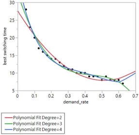
2.6.1 Study on the switching time . . . 42

2.6.2 Situation 1: deterministic phase-out returns with a constant phase-out return rate . . . 46

2.6.3 Situation 2: deterministic phase-out returns with an increasing phase-out return rate . . . 61

2.7 The value of phase-out returns . . . 72

2.8 Conclusion . . . 73

Chapter 3 Optimal policy structure and newsvendor-like heuristic policy with stochas-tic phase-out returns . . . 74

3.4 Observations and characterizations of the optimal policy . . . 78

3.5 Heuristic inventory policy development . . . 81

3.5.1 lm=lr =1 . . . 81

(9)

3.5.3 lm=1,lr =0 . . . 88

3.5.4 lm=0,lr =1 . . . 90

3.6.1 Situation 1: stochastic phase-out returns with a constant unit phase-out return probability . . . 93

3.6.2 Situation 2: stochastic phase-out returns with an increasing unit phase-out return probability . . . 100

Chapter 4 Analysis of the End-of-life Inventory for spare parts with incentives for phase-out returns . . . .108

4.4.1 Total cost savings from incentives . . . 110

4.4.2 Break-even points for the incentive unit costCI . . . 116

Chapter 5 Conclusions and future research. . . .122

5.2 Future research . . . 123

(10)

LIST OF TABLES

Table 2.1 Notation Summary . . . 14

Table 2.2 Values of parameters in base cases . . . 17

Table 2.3 The varied system parameters and their corresponding values in the numerical experiments . . . 41

Table 2.4 Values of parameters unchanged in the numerical experiments . . . 41

Table 2.5 Effect summary in the full factorial design withdr,CB O, andhr . . . 45

Table 2.6 Summary of fit in the full factorial design withdr,CB O, andhr . . . 45

Table 2.7 Effect summary in the single factor design with log₁₀(dr) . . . 45

Table 2.8 Summary of fit in the single factor design with log₁₀(dr). . . 46

Table 2.9 Summary of fit in the single factor design withdr . . . 47

Table 2.10 Switching times in lead time scenariolm=lr=1 whenrp o is constant . . . 49

Table 2.11 Performance of the heuristics in lead time scenariolm=lr =1 whenrp o is constant . . . 49

Table 2.12 Switching times in lead time scenariolm=lr=0 whenrp o is constant . . . 52

Table 2.13 Performance of the heuristics in lead time scenariolm=lr =0 whenrp o is constant . . . 52

Table 2.14 Switching times in lead time scenariolm=1,lr=0 whenrp ois constant . . . . 55

Table 2.15 Performance of the heuristics in lead time scenariol_m=1,l_r=0 whenrp o _is constant . . . 55

Table 2.16 Switching times in lead time scenariolm=0,lr=1 whenrp ois constant . . . . 58

Table 2.17 Performance of the heuristics in lead time scenariol_m=0,l_r=1 whenrp o _is constant . . . 59

Table 2.18 Switching times in lead time scenariolm=lr=1 whenr p o t is increasing . . . 62

Table 2.19 Performance of the heuristics in lead time scenariol_m=l_r =1 whenr_tp o is increasing . . . 62

Table 2.20 Switching times in lead time scenariolm=lr=0 whenr p o t is increasing . . . 65

Table 2.21 Performance of the heuristics in lead time scenariol_m=l_r =0 whenr_tp o is increasing . . . 65

Table 2.22 Switching times in lead time scenariolm=1,lr=0 whenr p o t is increasing . . . 67

Table 2.23 Performance of the heuristics in lead time scenariol_m=1,l_r=0 whenr_tp o is increasing . . . 67

Table 2.24 Switching times in lead time scenariolm=0,lr=1 whenr p o t is increasing . . . 70

Table 2.25 Performance of the heuristics in lead time scenariol_m=0,l_r=1 whenr_tp o is increasing . . . 71

Table 2.26 The cost increase percentages when phase-out returns are not recycled . . . 73

(11)

Table 3.4 The performance of three heuristics in scenariolm =lr =1 with a constant

unit phase-out return probabilityqp o _{. . . 94}

Table 3.5 The performance of three heuristics in scenariolm =lr =0 with a constant unit phase-out return probabilityqp o . . . 96

Table 3.6 The performance of three heuristics in scenariolm=1,lr=0 with a constant unit phase-out return probabilityqp o . . . 97

Table 3.7 The performance of the heuristic in scenariolm=0,lr=1 with a constant unit phase-out return probabilityqp o _{. . . 98}

Table 3.8 The values of the increasing unit phase-out return probabilityq_tp o during the final phase . . . 100

Table 3.9 The performance of three heuristics in scenariolm=lr=1 with an increasing unit phase-out return probabilityq_tp o . . . 100

Table 3.10 The performance of three heuristics in scenariolm=lr=0 with an increasing unit phase-out return probabilityq_tp o . . . 101

Table 3.11 The performance of three heuristics in scenariol_m=1,l_r=0 with an increasing unit phase-out return probabilityq_tp o . . . 104

Table 3.12 The performance of three heuristics in scenariolm=0,lr=1 with an increasing unit phase-out return probabilityq_tp o . . . 105

Table 4.2 Total costs without incentives and with incentives at various incentive unit cost values (C_I) . . . 112

Table 4.3 Percent reduction in total costs for various incentive unit cost values (CI) . . . . 112

Table 4.5 The fixed system parameters and their corresponding values in the numerical experiments . . . 113

Table 4.6 Economical savings when the incentive option is available andCI=12.5 . . . . 113

Table 4.7 Economical savings when the incentive option is available andCI=7.5 . . . 114

Table 4.8 Economical savings when the incentive option is available andCI=2.5 . . . 114

Table 4.9 Economical savings when the incentive option is available andCI=0 . . . 114

Table 4.10 Break-even points forCI in the scenariolm=lr=1 . . . 117

Table 4.11 Break-even points forCI in the scenariolm=lr=0 . . . 118

Table 4.12 Break-even points forCI in the scenariolm=1,lr=0 . . . 119

(12)

LIST OF FIGURES

Figure 2.1 The inventory system with two stocking points for serviceable and repairable

inventories, respectively . . . 9

Figure 2.2 Timeline of events in one period whenlm=lr=1 . . . 10

Figure 2.3 Timeline of events in one period whenlm=lr=0 . . . 11

Figure 2.4 Timeline of events in one period whenlm=1,lr=0 . . . 11

Figure 2.5 Timeline of events in one period whenlm=0,lr=1 . . . 11

Figure 2.6 Manufacturing and repair quantities at 30 periods to go whenlm=lr=1 and serviceable inventory is 0 . . . 18

Figure 2.13 Manufacturing and repair quantities at 25 periods to go whenl_m=l_r=0 and serviceable inventory is 0 . . . 23

Figure 2.15 Manufacturing and repair quantities at 30 periods to go whenlm=1,lr=0 and serviceable inventory is 0 . . . 25

Figure 2.16 Manufacturing and repair quantities at 30 periods to go whenl_m=1,l_r=0 and serviceable inventory is 2 . . . 26

Figure 2.19 Manufacturing and repair quantities at 30 periods to go whenl_m=0,l_r=1 and serviceable inventory is 0 . . . 28

Figure 2.23 Best switching time with the change of demand rate . . . 43

(13)

Figure 2.25 Best switching time with the change of inventory carrying cost rate . . . 44 Figure 2.26 Regression of the best switching time on demand ratedr(dris log-transformed) 48 Figure 2.27 Regression of the best switching time on demand ratedr . . . 48 Figure 2.28 The distribution of cost deviations in Heuristic 1 in the scenariolm=lr=1

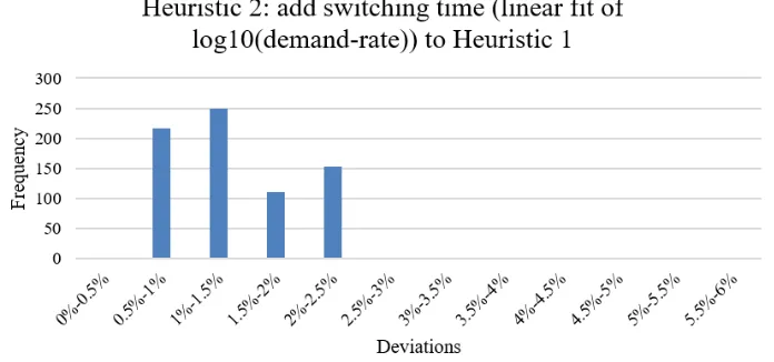
whenrp o _{is constant . . . 50} Figure 2.29 The distribution of cost deviations in Heuristic 2 in the scenariolm=lr=1

whenrp o is constant . . . 50 Figure 2.30 The distribution of cost deviations in Heuristic 3 in the scenariolm=lr=1

whenrp o _{is constant . . . 52} Figure 2.32 The distribution of cost deviations in Heuristic 2 in the scenariol_m=l_r=0

whenrp o _{is constant . . . 53} Figure 2.34 The distribution of cost deviations in Heuristic 1 in the scenariolm=1,lr=0

whenrp o is constant . . . 55 Figure 2.35 The distribution of cost deviations in Heuristic 2 in the scenariol_m=1,l_r=0

whenrp o is constant . . . 56 Figure 2.36 The distribution of cost deviations in Heuristic 3 in the scenariolm=1,lr=0

whenrp o _{is constant . . . 60} Figure 2.43 The distribution of cost deviations in Heuristic 1 in the scenariolm=lr=1

whenr_tp o is increasing . . . 63 Figure 2.44 The distribution of cost deviations in Heuristic 2 in the scenariolm=lr=1

(14)

Figure 2.48 The distribution of cost deviations in Heuristic 1 in the scenariolm=1,lr=0 whenr_tp o is increasing . . . 68 Figure 2.49 The distribution of cost deviations in Heuristic 2 in the scenariolm=1,lr=0

whenr_tp o is increasing . . . 68 Figure 2.50 The distribution of cost deviations in Heuristic 3 in the scenariolm=1,lr=0

whenr_tp o is increasing . . . 72

Figure 3.1 Manufacturing and repair quantities at 18 periods to go whenl_m=l_r=1 with 19 products in use and none in the serviceable inventory . . . 80 Figure 3.2 Manufacturing and repair quantities at 18 periods to go whenlm=lr=1 with

19 products in use and 1 part in the serviceable inventory . . . 80 Figure 3.3 The distribution of cost deviations in Heuristic 1 in the scenariolm=lr=1

whenqp ois constant . . . 95 Figure 3.4 The distribution of cost deviations in Heuristic 2 in the scenariol_m=l_r=1

whenqp ois constant . . . 95 Figure 3.5 The distribution of cost deviations in Heuristic 3 in the scenariolm=lr=1

whenqp o_{is constant . . . 95} Figure 3.6 The distribution of cost deviations in Heuristic 1 in the scenariolm=lr=0

whenqp o_{is constant . . . 97} Figure 3.9 The distribution of cost deviations in Heuristic 1 in the scenariolm=1,lr=0

whenqp ois constant . . . 98 Figure 3.10 The distribution of cost deviations in Heuristic 2 in the scenariolm=1,lr=0

whenqp ois constant . . . 98 Figure 3.11 The distribution of cost deviations in Heuristic 3 in the scenariolm=1,lr=0

whenqp o_{is constant . . . 99} Figure 3.12 The distribution of cost deviations in the heuristic in the scenariolm=0,lr=1

whenq_tp ois increasing . . . 101 Figure 3.14 The distribution of cost deviations in Heuristic 2 in the scenariolm=lr=1

whenq_tp ois increasing . . . 101 Figure 3.15 The distribution of cost deviations in Heuristic 3 in the scenariol_m=l_r=1

(15)

Figure 3.16 The distribution of cost deviations in Heuristic 1 in the scenariolm=lr=0 whenq_tp ois increasing . . . 102 Figure 3.17 The distribution of cost deviations in Heuristic 2 in the scenariolm=lr=0

whenq_tp ois increasing . . . 103 Figure 3.18 The distribution of cost deviations in Heuristic 3 in the scenariolm=lr=0

whenq_tp ois increasing . . . 103 Figure 3.19 The distribution of cost deviations in Heuristic 1 in the scenariolm=1,lr=0

whenq_tp ois increasing . . . 105 Figure 3.22 The distribution of cost deviations in the heuristic in the scenariolm=0,lr=1

whenq_tp ois increasing . . . 106

(16)

CHAPTER

1 INTRODUCTION

We investigate a problem faced by many original equipment manufacturers (OEM) of products that

are no longer manufactured but still under warranty. When the products break down, the OEM still has to provide technical support and guarantee the supply of usable parts to replace the broken parts

in these products. This problem exists for automobile, computer, aircraft, printer manufacturing

companies and others. After the regular production is terminated, the demand for spare parts is traditionally satisfied by the parts obtained from the last order/production batch, which is called

thelast-time buyin the literature.

Thefinal phaseorend-of-life phasestarts when the specific tooling used to produce the spare parts, is disposed; and it ends when there is no product in use or the last service contract ends. The

final phase can be as long as dozens of years for products in the aircraft and automobile industry. So

the initial inventory of spare parts from the last run can be very large and may have to be held for a long time. Too much inventory may incur obsolescence cost and high inventory cost for carrying

the unused spare parts. However, the lack of spare parts may incur expensive lost sales cost and

goodwill cost. The primary trade-off in this phase is balancing the risk of obsolescence and the risk of unmet service obligations.

In most cases, the manufacturer does not have full information about the demand for spare parts, so it is not possible to make a good estimate of how many parts to produce in the last production

batch. Thus, it is critical to propose some new strategies that can be applied to help with the inventory

(17)

In our research, we consider three alternative sources to obtain usable spare parts in the final

phase. The first source is phase-out returns from customers who trade in or return the old products due to a product upgrade or other reasons. The reusable parts are extracted from the phase-out

returns and can be used to satisfy the demand for spare parts from other customers. The second

source is through repair of returned defective parts. The third source is to produce new parts using an alternative production method, such as additive manufacturing for small batch production.

The objective of the dissertation is to develop efficient solutions that provide the optimal and

near-optimal heuristic policies to minimize the total cost incurred during the final phase. Phase-out returns play a significant role in our approach to this problem, however, there is no existing research

literature addressing the issue in depth. Therefore we investigate the effect of phase-out returns on

the inventory system.

In Chapter 2, the phase-out return rate is assumed to be known and deterministic, while the

demand for spare parts are stochastic. Based on the characteristics of this inventory control

prob-lem, a discrete-time Markov Decision Process (MDP) model is formulated to obtain the optimal policy. The optimal policy obtained from solving an MDP model consists of a list of manufacturing

and repair quantities in each possible state and period. However, solving an MDP model can be

cumbersome and time-consuming and the implementation of the solution is not simple or intuitive. Based on the characterization of the optimal policy, we propose newsvendor-like heuristic policies

that are near-optimal and easily computed.

In Chapter 3, the phase-out return rate is assumed to be stochastic. Obtaining the optimal policy

from solving the MDP model is theoretically possible, but may not be feasible in realistically-sized

problems due to the computational complexity. We introduce practical heuristics to replace the complicated and impractical optimal policies.

In Chapter 4, we introduce incentives for phase-out returns by which customers will be more

likely to return their outdated products to the manufacturer. We also quantitatively evaluate the economical cost savings from incentive decisions and provide recommendations for whether to

(18)

CHAPTER

2 OPTIMAL POLICY STRUCTURE AND

NEWSVENDOR-LIKE HEURISTIC

POLICIES WITH DETERMINISTIC

PHASE-OUT RETURNS

2.1 Introduction

With technology innovation, new generations of products enter the market to gradually replace

outdated products. Product life cycles, especially for durable products, can be as long as several decades. Since original equipment manufacturers (OEM) often have service contracts with their

customers, they must guarantee the supply of spare parts when the outdated products break down.

In practice it is common that the specified tooling for producing spare parts used to support products in the field is retired at a certain time due to economic concerns. Manufacturers may make

a final production run in order to build inventory to satisfy future demand. The final phase or

end-of-life phase of spare parts starts when the specified tooling is disposed after the final production run, and it ends when the products associated with the spare parts are no longer supported or out

of warranty. So in the final phase, a cheap and reliable source for re-supply is no longer available.

(19)

unmet service obligations. The literature addressing the end-of-life inventory problem extends back

to the 1960s[AD68]. There is, however, no existing model that can be applied directly to all our cases. In this research we consider a particular spare part for a product in the market place, such as a toner

assembly for a copier. We consider alternative sources of spare parts in the final phase.

The first source is phase-out returns from customers who trade in or return the old product due to product upgrade or other reasons. The reusable parts are extracted from the phase-out returns and

can be used to satisfy the demand of other customers. The number of phase-out returns in a specific

interval of time is dependent on the total number of products in the market place. Here we assume all the outdated product will eventually be returned to the manufacturer for recycling. The final

phase ends when the last product is returned. Alternatively, it could end when the manufacturer’s

contractual obligation to support the product ends.

The second source is through repair of returned defective parts. When a product breaks down,

the defective part will be replaced with a new part from serviceable inventory and returned back

to the manufacturer if it is repairable. Otherwise it is disposed. So the demand for a serviceable part is coupled with a return or disposal of a defective part. The returned defective parts are kept in

repairable inventory waiting to be repaired for future use.

The third source is to produce new parts using short-cycle time manufacturing, such as additive manufacturing for small batch production. Since the tooling for the traditional batch production

is disposed, manufacturing new parts using these tools is no longer possible. However, some new technologies, such as additive manufacturing, can replace this lost capacity[HH12]. We assume

obtaining new parts in the final phase is more expensive than repairing defective parts. However,

the goodwill cost of not satisfying the demand may be much more costly in the long-run from a manufacturer’s view. Thus it is worthwhile to adopt an alternative way to produce parts if possible.

Besides obtaining new parts from advanced technologies, there is also a possibility to get new

parts from some third party service providers. In fact, no matter whether new parts are obtained from short-cycle time manufacturing or third parties, the unit cost of getting a new part is generally

much higher than the unit repair cost. To simplify this problem, we do not differentiate between new

parts obtained from alternative production methods or third parties. In the following chapters, when we say a part is newly manufactured in the final phase, it can be either from advanced manufacturing

technology or third parties, which are both classified to be the third source.

Given the three sources above, many questions come to the surface. In this chapter, the inventory control questions we are concerned with are as follows.

1. What is the optimal repair and manufacturing policy in the final phase? In other words, when

and how many parts should be repaired or manufactured?

2. How do we handle the computational complexity of the problem? If generating the optimal

(20)

quickly compute good solutions?

With these questions in mind, we create a finite-horizon Markov decision process (MDP) model to obtain an analytical inventory control strategy on repair and manufacturing decisions. The

optimal policy can be obtained for small cases in a reasonable time, but not for larger versions of

the problem. We characterize the optimal results and create newsvendor-like heuristic policies. Experimental results indicate that the performance of the heuristic policies is quite good and the

heuristic policies have the potential to be used efficiently for large-size problems.

The rest of the chapter is organized as follows. Section 2.2 reviews the related literature. Section 2.3 describes the problem in detail and develops the MDP models. In Section 2.4, we observe

and characterize the optimal policy obtained from solving the MDP models in different lead time

scenarios. In Section 2.5, we propose heuristic methodologies and describe the details in four lead time scenarios. In Section 2.6, we show the results of numerical experiments to evaluate the

performance of the heuristic polices in different situations. In Section 2.7, we state the cost savings

from including phase-out returns as one of the three sources of the serviceable inventory. In the end, we summarize the results and discuss our conclusions in Section 2.8.

2.2 Literature review

In this literature review, we focus on the spare part inventory problem in the final phase. The

final phase of a spare part service life cycle is also referred as the end-of-life phase. This phase

starts immediately after terminating the traditional production of a product[For80]. Although the sale of a product is discontinued, there is an installed base to be serviced. In the literature, this

problem is known as the end-of-life (EOL) inventory problem, the final-buy problem (FBP), or the

end-of-production (EOP) problem.

The traditional tactic is purchasing or producing a sufficient volume of the spare parts to sustain

the need of the product in its remaining life time; this is called a life-time buy or last-time buy (LTB)

[JRM71].

When stopping production, the manufacturer has to decide on the lot size in the final production

run to cover spare part demand during the end-of-life phase. Although the unit production cost is relatively low, this tactic results in high holding cost and a low level of flexibility. There is a trade-off

between part availability and the cost of part obsolescence. So it is very important to determine

how many parts to stock.

This decision can be supported by forecasting expected spare part demand in the future based

on the installed base of the product. The installed base is the set of systems/products for which an

(21)

et al.[Lei14]consider the possibility of a contract extension when making the final order decision.

There are other alternative sources of supply that can supplement but complicate the decision on the LTB. In recent years, due to growing environmental concerns as well as economic

bene-fits, manufacturers seek to incorporate recovery activities into their processes. Product recovery

management encompasses the management of all used and discarded products, components, and materials that fall under the responsibility of a manufacturing company[Lei14], like recycling (reuse

of the material), repair (return used products to ”working order”) or remanufacturing (upgrade a

used product such that it is as good as a new one)[Thi95a]. This strategy is also used together with last-time-buy[Beh15a].

Many researchers have studied inventory management for product recovery. Thierry et al.[Thi95b],

and Ahiska and King[AK09; AK10a; AK10b]investigate inventory control strategies for a single product manufacturing/re-manufacturing system with state-dependent product returns. Simpson

[Sim78]describes a stochastic model for a one-product recovery system and proves the optimal solution structure for zero lead times and two stocking points. The model is extended by Inder-furth[Ind97]for the situation with positive lead times. Using these results, Kiesmüller and Scherer

[KS03]provide a method for the exact computation of the parameters which determine the optimal periodic policy and also proves two different approximations of the exact computation.

In an inventory system with product recovery, there are (at least) two inventories: the serviceable

inventory and repairable (recovered) inventory. The serviceable inventory is depleted by demand for serviceable parts and is replenished by repairing units available in the repairable inventory and/or

by producing/purchasing new units. The repairable inventory is depleted by repairing units for

serviceable inventory and/or by disposal and is replenished by defective units returned by users. Thierry[Thi95a]reviews the existing body of literature on repairable inventory, examines the various

models proposed and the major assumptions made in these models, and classifies them according to

their solution methodology – single versus multi-echelon, and exact versus approximate solutions. In a spare part repairable inventory system, there is complete dependence between the demand

for serviceable parts and the return of repairable parts as all failing units are replaced by serviceable

units. Since the repairable parts are usually not enough to satisfy all the demand in the final phase, the product recovery strategy should only one of the sources of spare part inventory supplies.

Allowing for the complexity of this problem, different heuristic approaches have been proposed

given different assumptions about product recovery. Kleber and Inderfurth[KI07]provide a promis-ing new heuristic approach for determinpromis-ing the final order size and dynamic remanufacture-up-to

levels, which yields near-optimal results in a small numerical study. Kooten and Tan[KT09]build a

transient Markovian model to represent the final order problem for a repairable spare parts with a certain repair probability and repair lead time. Behfard et al.[Beh15b]develop a heuristic method

(22)

Another source to get parts in the final phase is to extract reusable parts from phase-out returns.

Phase-out returns are obtained from customers that do not want to keep the outdated products due to product upgrade or other reasons. Krikke and Laan[KL11]are the first groups of researchers to

introduce phase-out returns in end-of-life inventory management. In their paper, the products in the

final phase can be serviced by three ways: new parts obtained from a last-time buy, repaired failed parts, and phase-out returns. They propose a heuristic generic model in a case study and obtain a

control policy. Motivated by the study of Krikke and Laan[KL11], Pourakbar et al.[Pou14]take a

fully analytical approach to characterize the structure of the optimal policy and also investigates the value of phase-out information.

Other alternative policies, including offering customers a new product of the similar type or a

discount on the next generation product, have also been used in practice. For example, in consumer electronic products, there is typically considerable price erosion while the repair cost stays steady

over time. As a consequence, there might be a point in time at which the unit price of the product

drops below the repair cost. If so, it is more cost-effective to adopt an alternative policy to meet service demand toward the end of the final phase. Pourakbar et al.[Pou12]develop an expression for

the expected total cost function, which can be used to determine the optimal final order quantity

and switching time from repair to the alternative policy.

There are many variations of alternative policies. For example, Kleber et al.[Kle12]propose a

buy-back option which is to buy back failed products in order to improve the control of demand for spare parts and supply of recoverable parts. Cole et al.[Col16]introduce two types of trade-in

programs: one is a full trade-in policy where the firm issues a one-time offer to the entire population

that has the product under warranty, and the other is a matching trade-in policy where the firm issues a trade-in offer to a fraction of the warranty population in each period. Their analysis shows

that the savings from the use of a trade-in program can be significant and the full trade-in policy is

likely to be preferred over a matching trade-in policy.

Even though regular production is terminated in the final phase, some advanced technologies,

such as additive manufacturing (AM), can be used to get new parts to supplement the inventory.

Some researchers have already noticed the potential applications of AM in logistics and supply chain management. Knofius et al.[Kno16]develop a method to increase the transparency in the

decision-making process through which spare part management may benefit from AM. This increases the

effectiveness and efficiency of identifying supported business cases and thus may support the adoption of AM in after-sales service supply chains. Attaran[Att17]examines some of the potential

benefits of AM in challenging traditional manufacturing constraints and its impact on the traditional

and global supply chain and logistics. Khajavi et al.[Kha14]evaluate the potential impact of additive manufacturing improvements on the configuration of spare parts supply chains. Li et al.[Li17]

investigate the impact of AM on spare parts supply chains. They compare the total variable cost

(23)

centralized AM-based supply chain, and a distributed AM-based supply chain.

The above sources to obtain spare parts are characterized by different costs and flexibility prop-erties. It seems that a combination of different sources are promising but challenging. For example,

Inderfurth and Mukherjee[IM08]propose a heuristic method to find the optimal combination of the

three sources: the final lot of regular production, extra production runs, and using remanufacturing to gain spare parts from the used products.

To the best of our knowledge, our research has not been considered in the literature. There

are certain aspects that distinguish our work from others. First, we introduce the combination of product recovery, phase-out returns and new production runs (e.g. by using AM) in this end-of-life

inventory problem for spare parts, which has not been discussed in the previous literature. Second,

the length of the final phase is directly dependent on the phase-out returns. While some researchers have noted this, they do not provide any analysis or practical strategies. We consider the time length

of the final phase, propose an exact solution, and create implementable heuristic approaches based

on the characterization of the optimal control policy. Third, our heuristic approaches have the potential to be generalized to larger examples and they are not strictly limited to certain special

cases.

2.3 Problem description and formulation

We are concerned with a single spare part type for an aging product deployed and serviced in the

field. The product has reached the point in its lifecycle where the regular production of this product has ceased. However, the manufacturer still has to maintain an inventory of spare parts to satisfy

the demand of customers who are still using the product. This serviceable inventory comes from

the combination of the following three sources.

The first source is from the repair of failed parts coming from the field. In this case, usable spare

parts are stocked in the serviceable inventory, while the failed parts are stored in the repairable

inventory until repair operations are performed to convert the parts to serviceable inventory. The second source is the manufacturing of new parts from an alternative and typically more expensive

source such as using additive manufacturing technology. The last source is extracting usable parts

from phase-out returns, which are old products/systems retrieved from customers who do not want to use the old products/systems anymore. If the phase-out returns are in good condition, we assume

all usable parts extracted from these returns can be used directly and they are placed directly into

the serviceable inventory; otherwise, the extracted parts are placed into the repairable inventory. As these phase-out returns reduce the size of the installed base, future demand for spare parts are

also reduced when more phase-out products have been returned to the manufacturer. In this chapter, we assume the manufacturer provides life-long support to the products until all old products in the

(24)

The system is modeled as a stochastic manufacturing/repair system with two stocking points:

serviceable inventory and repairable inventory, as illustrated in Figure 2.1. In our problem, both serviceable inventory and repairable inventory have finite capacities. When the inventory is full,

incoming parts are disposed. In addition, serviceable inventory can have a negative lower limit,

indicating the ability to backorder unmet demand for spare parts.

Figure 2.1The inventory system with two stocking points for serviceable and repairable inventories, re-spectively

As described above, the serviceable inventory includes spare parts which can be used directly

as replacements to failed parts in defective products while repairable inventory includes defective

spare parts awaiting repair, i.e., conversion to serviceable inventory. Whenever a spare part in a product in use breaks down, the defective one is replaced with a part from serviceable inventory.

If the replaced defective part is repairable, it is added to the repairable inventory; otherwise, it is

disposed of directly. So it is noted that each demand of a new part is coupled with a defective return. In the following analysis, we assume that all defective parts are repairable.

If there are no available useable parts in serviceable inventory when a product breaks down, then

the product is either in a state of "backorder" or "lost-sales" depending on the status of serviceable inventory. If the serviceable inventory has not reached the lower bound (the lower bound is usually

a negative value indicating the capacity to hold backordered products), then the product is on

"backorder" and the need of a useable part for this product will be satisfied by the future repair and manufacturing orders. Otherwise, the product is on "lost-sales" and will never be fixed. In this

chapter, the lower bound of serviceable inventory is set to be large enough in absolute value to avoid

the lost sales in the final phase.

The problem is to find the optimal policy that defines how many parts to repair or manufacture

(25)

if it provides the smallest expected cost during the final phase.

The system is formulated as a finite discrete-time Markov decision process (MDP)[How60]. A Markov decision process is a stochastic sequential-decision model that is defined by a set of

system states, a set of decisions to make, an immediate reward function to optimize and a transition

probability matrix that defines the probability of going from one state to another in one transition under a given decision.

The model is based on periodic review with four lead-time combination scenarios, i.e. the

scenario where manufacturing and repair lead times are both one period (lm=lr=1); the scenario where both lead times equal zero (lm =lr =0); the scenario where repair lead time is zero and manufacturing lead time is one period (lm=1,lr=0 ); and the scenario where repair lead time is 1 and manufacturing lead time is zero (l_m=0,l_r=1 ); In all scenarios, it takes one time period for the phase-out returns to be delivered to the manufacturer.

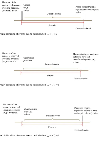
Before introducing the details of the MDP model, we specify the order of events occurring in

each period in Figures 2.2, 2.3, 2.4, and 2.5. For example in Figure 2.2, this timeline is based on the assumption that both lead times for manufacturing and repair operations are one period. The

events during a single period occur following the order below:

Figure 2.2Timeline of events in one period whenlm=lr=1

1. The state of the system (serviceable inventory, repairable inventory) is observed; and the

phase-out products are shipped to the manufacturer.

2. Decisions (repair and production quantities) are made;

3. Demand occurs and repairable defective parts are received;

4. Costs (manufacturing cost, repair cost, holding costs for both serviceable and repairable

(26)

Figure 2.3Timeline of events in one period whenlm=lr=0

Figure 2.4Timeline of events in one period whenlm=1,lr=0

(27)

5. The orders in step 2 arrive and are placed in serviceable inventory along with any phase-out

returns; any returned defective parts from step 3 are placed into repairable inventory.

When the lead time for repair (lr) or manufacturing (lm) operations changes from 1 period to 0 ,

then the repair order or manufacturing order or both are received immediately at the beginning of

each period, i.e., before step 3 above.

2.3.1 State space

The state at the beginning of periodt is represented by two variables: serviceable inventory level,

It (i.e., on-hand serviceable inventory minus backorders) and repairable inventory,Jt. Thus, the state of the system (St) is represented by the ordered pair of state variables, i.e.,St = (It,Jt). The inventories are bounded as indicated below:

I_min≤It≤Imax (2.1)

0≤Jt ≤Jmax (2.2)

IfImin<0, backordering of demand up to−Iminunits is allowed.

The final phase starts at time 0, and ends at timeT. Thus the finite horizon in this problem is [0,T]. In this periodic review inventory system, the final phase is broken down into time intervals, i.e., periods. The optimal sequence of decisions solved by an MDP model is in the reverse order.

For example, the decision made at timet is followed by the decision at timet −1 in the optimal

sequence of decisions. So it is desirable to describe the sequence decision in the time reverse order. We use "t periods to go" to represent the remaining time until the end of the final phase. Thus the

tthperiod is "T −t periods to go".

2.3.2 Decision space

The decisions to be made are how many parts to repair (p) and manufacture (m) during each period

based on the system stateSt at that time. Clearly, the feasible pairs of manufacturing and repair

decisions for a state should be determined considering the stock capacity of the system, as well as the manufacturing and repair capacities. Here, we assume there is no limit on the repair capacity as

long as there are enough defective parts to repair in the repairable inventory.

2.3.3 State transition and transition probabilities

The state transition from one period to the next depends on the manufacturing and repair decisions

made, as well as customer demand for spare parts and phase-out returns that occur during the

(28)

andp, respectively, and the demand and phase-out returns during periodt,Dt andRt , take on the

valuesd andrp o, respectively, then the next state isSt+1= (It+1,Jt+1). Time periodt is within[0,T]. In the lead time combination scenario where manufacturing and repair lead times equal one

period (lm=lr=1), the serviceable and repairable inventories at the end of each period (or at the beginning of the next period) are shown below:

It+1=min{max{It−d,Imin}+m+p+rp o,Imax} (2.3)

Jt+1=min{Jt−p+d,Jmax} (2.4)

In the case where where both lead times equal 0 (lm =lr =0), the serviceable inventory at the beginning of the next period (I_t₊₁) changes:

It+1=min{max{It+p+m−d,Imin}+rp o,Imax} (2.5)

In the case where repair lead time is zero and manufacturing lead time is one period (lm=1,lr=0), the serviceable inventory at the beginning of the next period (It+1) changes:

It+1=min{max{It+p−d,Imin}+m+rp o,Imax} (2.6)

In the case where repair lead time is one period and manufacturing lead time is 0 (l_m=0,l_r=1), the serviceable inventory at the beginning of the next period (It+1) changes:

It+1=min{max{It+m−d,Imin}+p+rp o,Imax} (2.7)

The transition probability from stateSt toSt+1under a pair of decisions(m,p), represented by P(St,St+1,(m,p)), is equal to the sum of the joint probabilities of occurrence for the demand and phase-out returns,(d,rp o), which lead to transition fromSt toSt+1under the decision(m,p), as indicated below.

P(St,St+1,(m,p)) =

X

(d,rp o₎_∈_A(m,p) St→St+1

P(Dt =d,Rt =rp o) (2.8)

whereA_St(m_→,p_St)₊

1 is the set of all pairs of demand and phase-out returns that cause a transition from St toSt+1under the decision(m,p).

2.3.4 Reward function

The reward function is defined as the expected cost per period which consists of fixed and variable manufacturing and repair cost, holding cost for serviceable and repairable inventories, backorder

(29)

Table 2.1Notation Summary

Notation Definition

SM Setup cost for manufacturing operations SP Setup cost for repair operations

CM Manufacturing cost per unit CP Repair cost per unit

hr Inventory carrying cost rate ($/$ inventory/unit time) CH S Holding cost per serviceable unit per period

CH R Holding cost per recoverable unit per period CB O Backorder cost per unit per period

CLS Lost sales cost per unit

C_DISPs Disposal cost for serviceable items per unit C_DISPr Disposal cost for repairable items per unit

DISPs_t Disposal amount of serviceable items during periodt DISPr_t Disposal amount of repairable items during periodt LSt Lost sales quantity during periodt

B_t Backordered demand during periodt Nt Installed base at the beginning of periodt. I_minser Lower bound of serviceable inventory Iser

max Upper bound of serviceable inventory Imaxrep Upper bound of Repairable inventory

used in the cost function.

Given that the system is in stateSt, the manufacturing and repair decisions taken aremandp,

respectively, the demand isd units andrp o units phase-out products are returned during periodt,

the reward function in a single periodt is calculated as:

C(St,m,p,d,rp o) =δ(m) +γ(p) +CH S[It+1]++CH RJt+1+CB OBt+CLSLSt+CDISPs DISP s t

+C_DISPr DISPr_t (2.9)

where the terms represent manufacturing cost, repair cost, holding cost for serviceable inventory, holding cost for repairable inventory, backorder cost, lost sales cost, disposal cost for servicebale

and repairable inventory, respectively.

The expressions for each term in Equation 2.9 are below.

(30)

The manufacturing cost and the repair cost are unchanged in different lead time cases:

δ(m) =







SM+CM·m, m>0

0, m=0

, γ(p) =







SP+CP·p, p>0

0, p=0

(2.10)

In the case where manufacturing and repair lead times equal one period, the backorder cost in

periodt is:

Bt =







−max{It−d,Iminser}, ifIt<d

0, otherwise

(2.11)

In the case where where both lead times equal 0, the backorder cost in periodt is:

B_t =







−max{It+m+p−d,I_minser}, ifIt+m+p<d

0, otherwise

(2.12)

In the case where repair lead time is zero and manufacturing lead time is one period, the backorder cost in periodt is:

Bt =







−max{I_t+p−d,I_minser}, ifI_t+p<d

0, otherwise

(2.13)

In the case where repair lead time is one period and manufacturing lead time is zero, the backorder

cost in periodt is:

Bt=







−max{It+m−d,Iminser}+p, ifIt+m<d

0, otherwise

(2.14)

In this chapter, lost sales only occur when unsatisfied demand exist when the final phase ends

— the serviceable inventory is a negative value at the end of the final phase — since we set up the

lower bound of serviceable inventory to be large enough in absolute value so the all the unsatisfied products are backordered rather than resulting in a lost sale.

The disposed usable parts and defective parts are below:

DISPs_t=







I_maxser −(It+m+p−d), It+m+p−d >Imaxser

0, It+m+p−d ≤I_maxser

(31)

DISPr_t =







Imaxrep −(Jt−p+d), Jt−p+d >I rep max

0, Jt−p+d ≤Imaxrep

(2.16)

Equations 2.15 and 2.16 stay unchanged in different lead time scenarios, since all unmet demand is

backordered rather than lost.

In this chapter, the repair and manufacturing orders are made based on the serviceable inventory

and repairable inventory. It is obviously not economical to overproduce any parts to incur disposal

cost for extra parts, so the disposal actions do not happen during the final phase.

Then, the expected cost in periodt is calculated considering all possible pairs of demand and

phase-out returns:

E[C(S_t,p,m)] =X rp o

X

d

P(D_t=d,R_t=rp o)·C(S_t,m,p,d,rp o) (2.17)

At the end of the final phase, there are lost sales cost, disposal cost for serviceable and repairable inventories if there are backorders, extra usable or defective parts left in the inventories.

So the cost function at the end of the final phase is below:

C(I_end,J_end) =CLS·Iend·1Iend<0+CDISPs ·Iend·1Iend≥0+C r

DISP·Jend (2.18)

where 1E is an indicator function that equals 1 if the eventE happens and 0 otherwise.

2.4 Observations and characterizations of the optimal policy

To better understand the problem, we propose an example for each lead time combination scenario,

create the corresponding MDP model[How60], and make some observations about the optimal policy. The examples in this section are base cases and the heuristic policies we create in Section 2.5

are based on the observations from the base cases in this section.

The parameters and their values in the base scenario are given in Table 2.2. The capacity of serviceable inventory or repairable inventory is defined by an upper bound (UB) and a lower bound

(LB).

The assumptions in this example are as follows:

• The demand for usable spare parts in the periodt is binomially distributed with the parameters dr andNt−rp o. The demand values with probability less than 0.001 are ignored to reduce

computational loads.

(32)

Table 2.2Values of parameters in base cases

Parameters Notation Values

Manufacturing cost per unit CM 10

Repair cost per unit CR 5

Backorder cost per unit CB O 100

Lost sales cost per unit CLS 187.5

Holding cost per unit for repairable inventory CH R 0.0192 Holding cost per unit for serviceable inventory CH S 0.0385

Annual holding cost rate hr 0.2

Serviceable inventory disposal cost C_DISPs 4

Repairable inventory disposal cost C_DISPr 2

Lower bound of serviceable inventory I_minser -30

Upper bound of serviceable inventory Iser

max 30

Upper bound of Repairable inventory Imaxrep 30

Phase-out return rate (phase-out return quantity per period) rp o 1 Demand rate (unit demand probability in the demand process) dr 0.2

Production capacity M 80

Initial intalled base (total products in use at time 0) N0 30

Length of the final phase T 30

• The lead time for phase-out returns is 1 period.

• All defective parts are repairable. So each demand for a serviceable part is coupled with a defective part returned.

• There is no setup cost for repair and manufacturing.

• All phase-out returns are in good condition unless all products in use are in need of spare parts which are on backorder, i.e., products in good condition are phased out and returned

first before backordered products.

• The usable parts extracted from phase-out products in good condition are placed in the serviceable inventory.

It is noted that the length of the final phase is directly dependent on the phase-out return rate

rp o, which is defined as the phase-out return quantity in each period. When there is no product

in the market, the return rate reaches 0 and the final phase ends. In this example, the phase-out return rate is constant and equal to 1 and a total of 30 products are available in the market when this

(33)

After solving the MDP model in each base case, the optimal policy yields a large table showing

how many defective parts to repair and how many new parts to manufacture in each period for each possible state. The optimal decision in a given period and state is defined as the repair and

manufacturing quantities combination that generates the lowest expected total cost.

We characterize the optimal policies obtained by solving the base cases in four lead time com-bination scenarios, respectively. It should be noted that the optimal decisions made in an MDP

model are obtained in a reverse chronological order. Again, we use the expression "t periods to

go" to indicatet time units remaining to the end of the final phase. For example, when we say 30 periods to go, it means there are 30 time units remaining to the end of the final phase.

2.4.1 lm=lr =1

When manufacturing and repair lead times are 1, the manufacturing and repair orders are received

at the end of each period. Figures 2.6 and 2.7 show optimal manufacturing and repair quantities at 30 periods to go when serviceable inventory(I)is 0 and 2 respectively and repairable inventory(J) ranges from 0 to 30. Figures 2.8 and 2.9 do the same when there are 25 periods to go.

Figure 2.6Manufacturing and repair quantities at 30 periods to go whenlm =lr =1 and serviceable

inventory is 0

In Figure 2.6 at 30 periods to go and no serviceable inventory, the horizontal axis ranges from 0 to 30 indicating the repairable inventory. The manufacturing quantities are shown as the height of the

blue rectangles; the repair quantities are shown as the height of the red rectangles. The interpretation

(34)

inventory is 2

(35)

inventory is 2

1. Observe the serviceable and repairable inventories (the serviceable inventory is always 0 when

the repairable inventory changes from 0 to 30).

2. If the serviceable inventory is less than 22, repair defective parts to bring the serviceable inventory up to 22. There may not be enough repairable parts, so the targeted inventory level

22 may not be reached.

3. If the serviceable inventory is less than 16 after the repair quantity in step 2 is added to it,

manufacture enough new parts to raise the serviceable inventory up to 16.

So there are two important base stock levels in the steps above: repair-up-to level (R0) and manufacture-up-to level (M₀), which are 22 and 16, respectively, for 30 periods to go (t =0).

When there are two parts in the serviceable inventory and the time period is unchanged (30

periods to go) in Figure 2.7, we can see that the optimal quantities of repair and manufacturing follow the same strategy and the two important base stock levelsR₀andM₀stay the same as Figure

2.6. The height of the green rectangles indicate the serviceable inventory levels.

When there are 25 periods to go and serviceable inventory is 0 and 2, respectively, the optimal quantity of repair and manufacturing shown in Figures 2.8 and 2.9 follow the same strategy but

the repair-up-to level and manufacture-up-to level decrease to 18 and 13, respectively. This is

reasonable since fewer products are being used in the market and demand for spare parts decreases correspondingly.