Predicting Parallel Applications’ Performance Across Platforms Using Partial
Execution
Tao Yang
∗Xiaosong Ma
∗ †Frank Mueller
∗Abstract
Performance prediction across platforms is increasingly important in today’s diverse computing environments. As both programs and their developers face unprecedented wide choices in execution platforms, cross-machine execu-tion time predicexecu-tion with reasonable accuracy equally ben-efits scheduling decisions of grid jobs as well as scientists in their research and development planning.
In this paper, we investigate an affordable method approaching cross-platform performance translation, based on the notion of relative performance between two platforms. We argue that relative performance can often be observed without running a parallel application in full. This paper shows that it suffices to observe very short partial
ex-ecutions of an application since most parallel codes are
it-erative and behave in a predictable manner after a minimal startup period. This prediction approach is observation-based and does not require program modeling, code anal-ysis, or architectural simulation. Our performance results (using four real-world parallel simulation codes and a to-tal of ten parallel machines with eight distinct architectures) demonstrate that performance prediction derived from par-tial application executions can yield highly accurate results at a low cost.
1. Introduction
Users of high-performance computing (HPC) platforms tend to have access to more and more geographically dis-tributed computational resources. Unfortunately, both the resources and the applications in today’s distributed com-puting environment are highly heterogeneous and of great complexity. This makes it difficult to determine the resource usage of a specific application on a wide range of execution platforms. That information is essential in HPC users’ de-cision making when they need to choose a system to obtain access to (or to own) for running their programs, especially for long production executions. For example, it would be helpful to provide scientists with performance estimations
∗ Department of Computer Science, North
Car-olina State University, Raleigh, NC, 27695-7534
{tyang2,ma,mueller}@csc.ncsu.edu
† Computer Science and Mathematics Division, Oak Ridge National
Laboratory
of their applications on several large clusters before they de-cide which cluster to apply for allocations on, and further, how many service units to request on that cluster. Overly in-accurate estimations often cause users to run out of service allocation in the middle of their grant or leave a lot of ser-vice units unused when the grant expires, affecting their fu-ture allocation application.
The same information is also instrumental in helping a grid resource scheduler to efficiently schedule user jobs. A “meta-scheduler” would like to know how long a job will run on each participating site to improve global load bal-ance and overall job throughput. When the job is sched-uled to run at a specific grid-participating site, the local job scheduling system there also needs the job’s estimated max-imum execution time, which is used as a parameter in their scheduling algorithms [22, 27]. Overly inaccurate estima-tions here may result in excessive wait times in queues or in forced premature job termination (cancellation) during exe-cution.
For many parallel applications, computational resource usage on a given execution platform is correlated to their ex-ecution time on this platform. In this paper, we study cross-platform execution time predictionfor efficient and accurate resource usage estimation as an affordableutilityfor HPC users and grid schedulers.
There have been numerous studies on parallel programs’ performance prediction and many of them can work on mul-tiple platforms (see Section 4). These prior efforts have mostly focused on performance modeling or program sim-ulation. However, the size, diversity, and extensibility of today’s HPC environments pose new challenges that tra-ditional performance prediction approaches were not de-signed to address.
ex-ecution time. Such approaches normally require both ap-plication analysis and system parameter benchmarking, or architecture-specific simulator development.
In contrast, our main approach is observation-based performance prediction, where we enable very short “test drives” of the applications on multiple candidate platforms to quickly derive the execution time of much longer runs. The results of these test drives can be stored in a database for reusing in future predictions.
One of the key innovations of our work is its reliance on the novel concepts ofrelative performanceandpartial execution. We observe that HPC users often have one or morereference computersto develop and test applications. Consequently, our work investigatesinter-platform perfor-mance translation.
More specifically, this paper aims to answer the follow-ing questions through our empirical study:
• Can we predict the overall execution time of a large-scale application on atarget systemusing the combi-nation of its known performance on areference system and therelative performancebetween the two systems derived from a very short run of the application?
• How early in this application’s execution can we reasonably capture its cross-platform relative perfor-mance?
• Will this early observation produce valid predictions for applications with data sizes or complexity that dy-namically change as the computation progresses?
• Can we extrapolate the relative performance knowl-edge collected from partial executions to predict the application’s execution time in computing a different problem size or using a different number of proces-sors?
• Will the choice of a reference system be significant? I.e., when an application has known performance data on multiple systems, will we produce similar predic-tions when using different machines as the reference system?
Our results from four production-scale parallel simula-tion codes on ten different large parallel computers show very promising prediction accuracy and low prediction overhead: in most cases, with a short execution that takes 1% or less of the total execution time, we obtain an over-all execution time prediction accuracy of 97% or higher.
The rest of the paper is organized as follows. Section 2 describes our prediction methods and performance trans-lation algorithms. Section 3 presents experimental results. Section 4 summarizes related work and Section 5 concludes the paper.
2. Methodology and System Design
Scientific applications generally have computationally intensive kernels. The performance of such applications is often constrained by the floating point resources avail-able, memory bandwidth, and the characteristics of inter-processor communication, via either shared memory or message passing. Due to these constraints, performance pre-diction is often challenging. At the same time, scientific ap-plications are characterized by their regularity in the course of executions, specifically with regard to array reference patterns (at the micro level) and alternating phases of com-putation and communication or I/O (at the macro level). It is this regularity that we exploit for our observation-based performance prediction, in contrast to traditional model- or simulation-based predictions.
The repetitive nature of scientific applications at the macro level is generally a property of the computational model that is based on the notion of convergence in dif-ferent mathematical approximation methods. Many, if not most, parallel applications aretimestep-based. In such ap-plications, a timestep is one step of computation followed by inter-processor communication to update data. Timestep computation is repeated until the results converge (e.g., when the simulation object reaches a stable state), or the computation has completed a given number of timesteps.
Traditional model-based or simulation-based approaches to performance prediction generally consider the entire exe-cution of an application and study the interplay between the program and the architecture in a case-by-case manner. For an observation-based approach, executing the entire appli-cation takes too long to be acceptable. Instead, our approach utilizespartial executionfor a limited number of timesteps to capture therelative performanceacross platforms for an application. We argue thatdue to the highly repetitive na-ture of scientific codes, the relative performance observed in this short partial execution is likely to sustain through the entire run. When used in conjunct with known full execu-tion time of a particular applicaexecu-tion on a reference platform, this result can then be utilized to perform cross-platform ex-ecution time predictions in a very cost-effective way.
2.1. Partial Execution
We have devised an API in support of partial execution for arbitrary applications on clusters. While the design was inspired by the properties of timesteps, the API can also be used in the absence of explicit timesteps — as long as the activities between two consecutive calls closely repre-sent repetitive phases in the application’s execution. In the rest of the paper, we use the term “timestep” when refer-ring to these periodic phases. The API for partial execution is as follows:
sets from secondary storage, this call should be used to separate initialization overhead from subsequent regu-lar timesteps.
• begin timestep(): This call identifies the beginning of a timestep and allows counters for metrics to be reset between timesteps.
• end timestep(maxsteps, rampsteps): This call indicates the end of a timestep and implements the logging of metrics pertinent to the timestep work. The first pa-rameter indicates the total number of timesteps before partial execution prematurely terminates the program’s execution. The second parameter indicates the number of ramp-up timesteps that should be ignored in the log-ging activity.
In practice, initialization is a one-time overhead typically with negligible cost to long-running applications, so the initialization call can often be omitted. If the ramp-up pa-rameter is not specified, our implementation uses a default value of 1, assuming the ramp up is finished by the sec-ond timestep. Excluding the first timestep allows caches to warm up before timing results enter the performance model. It also allows us to omit the initialization API call since ini-tialization overhead is incurred prior to any timings.
Partial execution utilizing this API allows one to ob-tain metrics on a per-timestep basis and limits the ber of timesteps an application executes. Once this num-ber is exceeded, the application will be terminated prema-turely. Hence, the objective of partial execution is not to ob-tain numerical results from scientific codes but to quickly and cheaply capture their rudimentary execution behavior.
The metrics obtained during partial execution can then be utilized to predict the performance of an application run across different platforms, as detailed below.
2.2. Cross-Platform Performance Prediction
Our approach of observation-based performance pre-diction is based on two sets of data, one from the refer-ence platform, where we have more performance knowl-edge about the application in question (denoted asA), andone from thetarget platform, where we want to predict the full execution time.
We assume that Tref, the full execution time of Aon the reference platform, ornum steps, the total number of
timesteps in the full execution, is available. This is reason-able considering that there is at least one “base platform” where the code is developed or tested, and researchers typ-ically keep track of the overall statistics for long-running jobs. In addition, we perform the same partial executions ofAon the reference platform as we do on the target
plat-form (see below).
On the target platform, we carry out a set of partial ex-ecutions ofAfor a limited number of timesteps. Both the
number of partial executions and the number of timesteps
per partial execution can be small, as will be demonstrated in the experimental section. The objective of the approach is to inflict minimal time overhead for any executions on both platforms so that performance predictions can be pro-vided quickly. This is especially important when scientists need to select their preferred target from a large set of can-didate platforms (based on relative performance,i.e., ma-chineM1isxtimes faster than machineM2). With known
execution times on the reference platform, one can further estimate the absolute performance to supply tight, yet rel-atively safe bounds on wall-clock time for their submitted jobs, long before having observed a complete run on the tar-get platform, which can takes hours or days.
Base Model: Our predictions are based on the average
per-timestep execution time for a set of repeated partial exe-cutions on the target platform to obtain the overhead per timesteptstepand the initializationtinit. The per-timestep averages from multiple runs are then averaged once more over the firstntimesteps,e.g., up to the number of timesteps within the partial execution. We call this “prediction using cumulative averages” (or running averages). The observed relative performance Rtar ref between the target and the reference platform can then be calculated using the result-ing average per-timestep overheadtavg step:
Rtar ref = ttar avg step
tref avg step
Equipped with the above observed relative performance and known execution timeTref on the reference platform, we can estimate absolute performance of Aon the target
platformTtar estas:
Ttar est=ttar init+Rtar ref×(Tref−tref init)
If Tref is not available but the total number of timesteps,
num steps, is known, we can estimateTtar estas:
Ttar est=ttar init+ttar avg step×num steps
The accuracy of the above estimation can be assessed by comparingTtar est, the predicted absolute performance of
A, withTtar, the measured performance on the target plat-form:
accuracy= Ttar est
Ttar
Obviously, when the initialization timetinitis very small in the overall execution time, the prediction accuracy ap-proximates the observed relative performance during the short partial executionsagainst the overall relative perfor-mance calculated from actual full executions on both plat-forms.
Filter Model: The base model of cumulative averages
suf-fices for simple applications and platforms without run-time/OS intervention that affects execution time. To further generalize the model to compensate for fluctuations in exe-cution time, a “filter model” is introduced next. The objec-tive of the filter model is to handle two types of commonly known fluctuations. First, initial fluctuations may occur for multiple timesteps, and not just for initialization code prior to the first timestep. Such fluctuations may be due to warm-up effects of resources, such as caches, but they can also originate from runtime/OS intervention, such as code and/or data migration to better utilize the resources of a given plat-form. Second, periodic fluctuations are common for addi-tional work performed everyk-th timestep, such as
check-pointing and I/O for visualization.
The filter model proposed in the following captures both initial and periodic fluctuations. During a partial execution, our API will perform online processing of collected per-timestep timing data. It calculates the ratio between each current timestep with the previousktimesteps and considers
the current fluctuation significant if this ratio differs from1
by a thresholdδor more. Bothkandδare tunable. In
prac-tice, we have found thatk = 5andδ = 0.05allow us to
identify both one-time anomalies and periodic I/O activi-ties.
Sliding Window Filter Model: We address recurring I/O
activities in our prediction by utilizing a sliding window of averages instead of cumulative averages. Intuitively, this method uses the average of timestep times collected in a contiguous window of sizew. Therefore, to ensure that we
include the correct proportion of computation and periodic activities, such as I/O, we need to use a window size that equals the observed period k. The difference between the
sliding window vs. the cumulative models materializes af-terwtimesteps. In the presence of I/O, the cumulative
ap-proach would be subject to periodic fluctuation while the sliding window provides stability.
With the filter and sliding window models, one of the challenges is to distinguish between random anomalies and periodic fluctuations. We apply heuristics (a) to compare partial execution times from multiple platforms (it is more likely an anomaly if it only occurs on one system) and (b) to detect recurring spikes/dips (it is more likely an anomaly if it only occurs once, especially close to the beginning of ex-ecution). If we detect such a one-time anomaly during par-tial executions, we treat it as a part of the one-time inipar-tial-
initial-ization cost and apply our prediction algorithm accordingly as described earlier in this section.
Because this prediction is observation-based, as long as
Ais executed in the same way across platforms, prediction
accuracy will not be affected by various system characteris-tics, such as different
• processor families, generations and clock frequencies, • bus interconnects (for shared-memory systems), • communication interconnects (for networked clusters), • memory and cache configurations,
• connections from compute nodes to shared disks, and • system software, such as operating systems and I/O
li-braries.
Our experiments in Section 3 demonstrate the above. In ad-dition, Section 3 presents irregularities in timestep execu-tion times due to system-dependent anomalies or recurring I/O activities, as well as our enhanced prediction models to handle these situations.
Of course, one major objective of our performance pre-diction scheme is always to minimize the overhead for par-tial executions. The question is,e.g., can we estimate the performance on the target platform using 64 processors with the relative performance observed in partial runs us-ing 8 processors only? The cheaper and more reusable the partial executions are, the higher we can expect the accep-tance of our approach to be by end users.
3. Performance Results
In this section, we present prediction accuracy and other results with our proposed approach using partial execution and the notion of relative performance. Some of the experi-ments were conducted using the partial execution APIs de-scribed in Section 2.1, while others were obtained from sci-entists who benchmarked per-timestep execution time for their applications. In the second case, we took the first n
timesteps to simulate partial executions.
3.1. Experiment Platforms
Our application performance data are collected from ten different parallel computers with eight distinct types of par-allel architectures. Table 1 summarizes their technical con-figurations.
3.2. Base Model and Relative Performance
We evaluated our partial execution method with two benchmarks from the DOE ASCI Purple suite [32], a set of novel applications comprising large-scale parallel codes with inputs resulting in hours of execution. This suite also comprises a mixture of scientific domains, types of meshes, and computation/communication models.
Name Location Architecture CPU No. nodes Procs/node Mem/node OS Shared FS Datastar-690 SDSC IBM SP4 1.7GHz Power4 8 32 128GB AIX GPFS Datastar-655 SDSC IBM SP4 1.5GHz Power4 176 8 16GB AIX GPFS Henry2 NCSU IBM Blade Center 2.8/3.0GHz Xeon 100 2 4GB Linux NFS
Ram ORNL SGI Altix 1.5GHz Itanium2 256 1 8GB Linux XFS
Turing UIUC Apple Xserver 2GHz G5 640 2 4GB Mac OS NFS Frost LLNL IBM SP3 375MHz Power3 64 16 16GB AIX GPFS Cheetah ORNL IBM SP4 1.3GHz Power4 27 32 32/64/128GB AIX GPFS Phoenix ORNL Cray X1 vector 512 1 2TB global UNICOS/mp StorNext Seaborg NERSC IBM SP3 375MHz Power3 380 16 16/32/64GB AIX GPFS TeraGrid NCSA Cluster 1.3/1.5GHz Itanium2 887 2 4/12GB Linux GPFS/NFS
Table 1.
the above platforms using 8 processors. These systems all yield fairly small performance variances, and our predic-tion results are based on 1-2 full execupredic-tions and 2-5 partial executions.
Figure 1. Sphot prediction accuracy using Datastar-690 as the reference platform
Figure 1 shows the prediction results for Sphot, using Datastar-690 as the reference platform and the other three systems as target platforms. For each platform, we portray two prediction methods: Steps, where the relative perfor-mance used in theith prediction point is based on the pair
of execution time values from timestepion the reference
and target platforms, andcumulative, where the relative per-formance is based on the cumulative average of execution times from timestep1toion both platforms.
In general, Figure 1 demonstrates that our prediction us-ing partial execution yields very accurate results: for all three target systems, the prediction error is within 1.5%. In addition, it demonstrates the following:(1)High
accu-racy can be reached at a very early stage of execution. Even with the first timestep, when initialization and warm-up ef-fects should perturb results on all three target platforms, the prediction accuracy is higher than 98%. Within 5 timesteps, the accuracy on all systems stabilizes at even higher accu-racy.(2)Partial executions can deliver accurate predictions
at a very low cost. In this full execution, Sphot executes
thousands of timesteps. On the most time-consuming plat-form (in this case Ram), the full execution took more than 11 hours while our partial execution of 25 timesteps only took 6 minutes. Moreover, as mentioned earlier our predic-tion model is accurate even with fewer timesteps as input. Therefore, a partial execution’s cost can be bounded by a small maximum wall time for a job. Even when this partial execution itself is terminated prematurely, our model still generates reasonable observation-based predictions.(3)The
“cumulative” method works better than the “steps” method by smoothing out small irregularities in per-timestep exe-cution times.(4)With such uniformly high accuracy, it
ap-pears that the selection of a reference platform is not impor-tant, at least for this code.
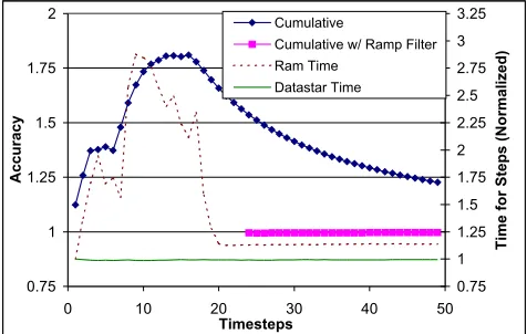
Figure 2. Normalized per-timestep execution time (right axis) and prediction accuracy (left axis) for sPPM
to perform page placement based on memory access pat-terns. As such, pages are moved to the node of most quently accesses to inflict lower latencies while less fquent accesses my result in longer latencies when being re-solved by remote memory accesses.
Our filter model can detect and compensate for this one-time overhead, as explained in Section 2.1. Figure 2 shows the difference in prediction accuracy with and without this “ramp filter”. With the non-discriminative cumulative av-erage method, the prediction error can reach 80%, and the effect of misleading relative performance lingers for many timesteps after the anomaly disappears. In contrast, with the improved prediction, the first 23 timesteps will not produce prediction results as they are classified as unstable. Right after that, the prediction instantly yields a consistently high accuracy of over 99%.
!"
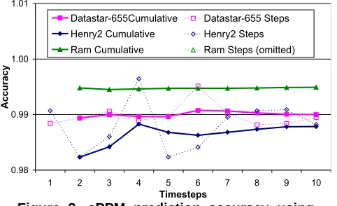
Figure 3. sPPM prediction accuracy using Datastar-690 as the reference platform
Figure 3 depicts the prediction accuracy for sPPM on all three target timesteps. Ram data points represent the first timestepsafterthe relative performance stabilizes us-ing the filter model. sPPM has far more expensive timesteps than Sphot, with each timestep taking around 3 minutes and full runs taking almost 10 hours on Datastar-690 and 655. Therefore, we run only 10 timesteps in our partial execu-tions. Again, the accuracy is remarkably high, at above 98% just after the first timestep.
Comparing the relative performance for Sphot and sPPM also reveals interesting facts. For Sphot, Ram is by far the worst platform, where each timestep takes more than 3.5 times as long as on Datastar-690. For sPPM, however, it is by far thebestplatform, where each timestep takes slightly more than 1/6 of the time on Datastar-690. This dramatic contrast is likely due to the different communication and computation patterns of the two codes. For example, sPPM uses frequent large messages, which may benefit from Al-tix’s distributed shared memory architecture. Such phenom-ena suggest that relative performance across platforms can vary dramatically from application to application (in this
case, a 20+ times difference). In addition, system parame-ters, such as the CPU frequency, do not offer significant in-formation: Ram and Datastar-690 happen to have the same CPU frequency.
Figure 4. sPPM with high I/O frequency on Ram and Henry2. The top figure shows normalized per-timestep times and the bot-tom one shows ratios between each current timestep time to the average of previous 5.
3.4. Sliding Window and Periodic I/O
Next, we consider predictions for executions with peri-odic I/O activities. Such periperi-odic I/O is very common in scientific codes for outputting intermediate results (a) for visualization and analysis and (b) for checkpointing cur-rent states to enable efficient restart if the execution is ter-minated unexpectedly. To save I/O time, most applications choose to periodically generate output every k
computa-tional timesteps. Between Sphot and sPPM, the latter pro-vides an easier interface to adjust this I/O frequency. The runs shown above used a default low I/O frequency. Fig-ure 4 depicts sPPM results from runs with a much higher I/O frequency (m= 10).
655 Conf. 8×1 4×2 2×4 1×8 Accuracy 1.002 0.991 1.012 1.004
Table 2. Accuracy in predictions for Datastar-655 runs using different
(number-of-processors-per-node × number-of-nodes)
combinations. The total number of proces-sors is fixed at 8.
655 Conf. 2×1 4×1 8×1 8×2 8×4 Accuracy 0.988 0.993 1.002 0.978 0.981
Table 3. Accuracy in predictions for Datastar-655 runs using different
(number-of-processors-per-node × number-of-nodes)
combinations. The total number of proces-sors varies from 2 to 32.
Figure 4 and Figure 5 depicts the I/O effect when the performance of sPPM is predicted from Ram to Henry2. This experiment serves a second purpose, namely to show that our ramp filter is valid on a reference platform as well. From the per-timestep timing curves shown in Figure 4, I/O “spikes” can be clearly identified after the execution stabi-lizes. On Henry2, where computation is faster than on Ram, I/O is significantly slower. Using our filter model that cal-culates the ratio of each current timestep versus the average of the previous 5 steps, we can successfully identify these I/O spikes as recurring behavior. We can also capturek, the
aforementioned periodic I/O frequency in terms of number of timesteps.
We address recurring I/O activities with thesliding win-dow model, as discussed in Section 2.2. Figure 5 shows the prediction results (after the initial noise is filtered out on the reference system). For the first 10 timesteps, the slid-ing window is growslid-ing, so the two models perfectly over-lap. After that, however, the cumulative algorithm shows a periodic fluctuation in accuracy while the sliding window algorithm is more stable.
We believe that the sliding window model will show more significant advantage if I/O is more frequent and of larger costs. If, however, I/O is sparse and of low cost, it may safely be disregarded by our identification algorithm at all. This is not a big issue though, as the I/O effect would not have a large impact on the overall prediction accuracy in the first place.
Finally, we study different processor/node configurations on the reference and target platforms. As mentioned ear-lier, our partial execution uses the same number of proces-sors and the same problem size as in the full execution. However, with today’s large SMP nodes, a practical con-figuration may not easily be reproduced on another plat-form. We subsequently assess the prediction accuracy with the cumulative average method from Datastar-690 (with
32-processor nodes) to Datastar-655 (with 8-32-processor nodes). On Datastar-690, we ran all experiments on one node. In the first group of tests, we fixed the number of processors at 8 and varied the number of nodes on Datastar-655 (1, 2, 4, and 8). In the second group of tests, we increased the total number of processors from 2 to 32, where we always tried to minimize the number of nodes to use on Datastar-655. As demonstrated by Table 2 and Table 3, the prediction ac-curacy remains high in both cases, with no significant vari-ance caused by the different processor/node configurations.
3.5. Application with Varying Timestep Overhead
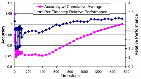
GENx is a multi-component rocket simulation code de-veloped at the University of Illinois [8]. The performance data we obtained are from model-validation runs simulating lab-scale rockets. We chose this particular simulation since it has an interesting property: the number of particles in its fluid dynamics code increases as time goes on. Therefore, unlike any other codes demonstrated in this paper, this per-timestep execution time grows gradually, reaching a factor of 1.8 at the final point (1550 timesteps in total). We use this code to determine if our model provides reasonable predic-tion in this situapredic-tion.
Figure 6. Per-timestep relative performance (right axis) and prediction accuracy with ac-cumulative average (left axis). There is one data point for each of the first 100 timesteps, and one for every 50 timesteps thereafter.
!
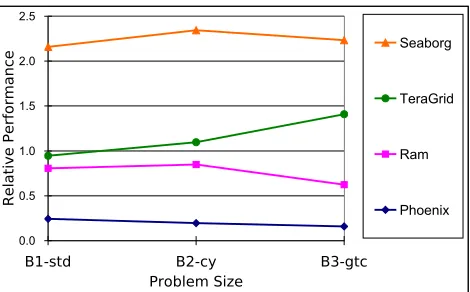
Figure 7. Gyro B1-std relative performance to Cheetah, using different number of proces-sors
of the firstntimesteps (n = 1,2, ...1550) is around 85%.
We still consider partial execution capable of delivering rea-sonable prediction accuracy for this type of codes with dy-namic complexity.
3.6. Extension: Application using Varying
Num-ber of Nodes and Inputs
GYRO [11] is a code for the numerical simulation of tokamak micro-turbulence solving time-dependent, nonlin-ear gyrokinetic-Maxwell equations. We obtained a large set of Gyro benchmarking results from ORNL and NCSU re-searchers who conducted Gyro runs with 3 problem in-puts (B1-std, B2-cy, and B3-gtc) on 5 platforms (Chee-tah, Ram, Phoenix, Seaborg, and Teragrid) using a vari-ety of processor numbers. Unlike the GENx simulation dis-cussed above, these Gyro runs produce extremely stable per-timestep time, and our prediction easily achieves very high accuracy. Again, the choice of the reference system among the five platforms does not appear to affect the pre-diction accuracy.
Instead of reporting the accuracy test results, we lever-age the abundance of experimental configurations in this case to explore the possibility of reusingthe relative per-formance data collected from a pair of partial executions to make predictions for runs using different number of proces-sors or different input data.
Phoenix Ram Seaborg Teragrid
# Pred. 11 6 5 7
Avg. Error 12.1% 25.5% 16.7% 25.8%
Table 4. Average errors caused by apply-ing the relative performance observed in 16-processor runs to runs using other number of processors
Figure 7 depicts the relative performance of four tar-get platforms against Cheetah using various number of
Figure 8. Gyro relative performance to Chee-tah, using 64 processors and different input problems
cessors (a multiple of 16, limited by hardware availabil-ity/configuration on each platform) to compute B1-std. We see that the level of consistency across different numbers of processors varies from platform to platform. Since using a small number of processors is likely to be cheaper (faster to get a job scheduled), we applied the relative performance observed in the run using the fewest processors (16) for each platform when predicting the overall execution time for the other process numbers. Table 4 shows the average predic-tion error, which varies between 12% and 26%.
Phoenix Ram Seaborg Teragrid Avg. Error 37.9% 17.0% 5.6% 23.2%
Table 5. Average errors caused by applying the relative performance observed in B1-std to B2-cy and B3-gtc
Figure 8 plots the relative performance across different problems, and Table 5 shows the average prediction error when we use the relative performance from computing the smallest input problem to predict for the other two prob-lems. This would also reduce the costs of partial executions. E.g., B3-gtc takes up to 3 times longer than B1-std. Here, the average error varies between 5% and 38%. Note that this group of Gyro results is not completely fair to our predic-tion method, as these several input problems not only bring different amount of computation, but also different compu-tation components to a certain degree.
application-specific data to give a quick “ball-park” estimate.
4. Related Work
Grid Job Scheduling: There has been an increasing
in-terest and efforts on grid scheduling (also called meta-scheduling) [14, 26, 29, 24], mostly built upon local job schedulers for executing jobs on distributed computing re-sources. It is recognized that job execution time is an im-portant resource specification item to be translated across machines. However, existing or under-development grid schedulers either do not offer execution time translation, thereby implying that users are responsible for specifying a “safe” maximum wall time value across machines, or they adopt simplified translation methods, such as stretch-ing the execution time with the CPU frequency ratio be-tween two machines [24], which is known to be very in-accurate. Other work on cross-platform performance pre-diction (e.g., Prophesy [30]) was mostly based on model-ing computational kernels instead of complex applications with diverse tasks. Our work can form a building block for future grid schedulers by offering affordable job execution time predictions for diverse applications and platforms.
Parallel Program Performance Prediction: There have
been numerous previous studies of performance prediction for parallel programs. Many of these studies are built upon performance modeling techniques (e.g., [1, 7, 10, 15, 21, 28, 31]) requiring either in-depth knowledge of the applica-tions to build analytical models (e.g., [2, 18, 25, 33, 34]) or special compiler/instrumentation tools to infer such knowl-edge from parallel codes (e.g., [4, 6, 12, 21]). With care-ful modeling of applications and platforms, many of these previous studies achieved high prediction accuracy. How-ever, detailed modeling often compromises the portabil-ity of prediction tools.E.g., some existing approaches are application-specific [2, 16] or language-specific [6, 12]. In addition, a number of prediction techniques are based on simulations (e.g., [3, 4]) where simulators are used to mea-sure the execution time of applications.
Most of the work mentioned above targeted perfor-mance prediction for the purpose of performance opti-mization. In contrast, our method targets performance pre-diction as a means for making resource usage estima-tion to help applicaestima-tion owners in their research planning and daily use of diverse computing resources. In such cases, users may not be able or willing to afford tradi-tional performance prediction techniques, which require a fair amount of work due to model building or instrumen-tation plus simulation. Especially today’s multi-component codes, such as the rocket simulation discussed in this pa-per, comprise modules from many application domains with diverse computational models/algorithms making an-alytical modeling very hard. Also, they often use exter-nal libraries (MPI, BLAS, PETSc, NetCDF, just to name a few), and/or multiple languages (e.g., mixed C/Fortran/C++
programming). This greatly decreases the feasibility and effectiveness of both analytical and compiler-aided per-formance modeling. Finally, given the large number of application-platform combinations in future grid environ-ments, simulation-based prediction can consume exces-sive system resources themselves. In contrast, we de-velop observation-based performance prediction, which does not require in-depth knowledge of parallel codes or systems. This makes our approach application-independent, language-independent, and platform-independent.
Further, many multi-platform performance modeling ef-forts (e.g., [3, 4, 5, 15, 20, 21]) evaluated their approaches with data collected at multiple supercomputers. However, data from each machine are processed individually, so are predictions and evaluations performed. Our approach, in-stead, combines benchmarking results from multiple plat-forms for cross-platform prediction.
Several recent studies addressed performance prediction in heterogeneous grid environments [13]. A few projects ad-dressed relative performance [16] and performance porta-bility [17, 23]. However, we are not aware of work on per-formance predictionbased onrelative performance.
Finally, the repetitive behavior of applications has been exploited in speeding up run times on architecture simu-lators [19] and predicting performance metrics based on history information [9]. Such studies exploit repetition at “instruction block” level while we exploit larger-scale and more explicit behavior repetition in high performance sci-entific codes, based on the iterative nature many of them possess.
5. Conclusion
In this paper, we demonstrated the benefit of a black-box style, observation-based performance prediction approach built on the notion of relative performance and utilizing af-fordable, short partial application executions. We believe the merits of this approach lie in itssimplicity,portability, andcost-effectiveness, making it ideal for performance pre-diction as a general service to HPC users and grid sched-ulers.
6. Acknowledgements
This work was supported in part by NSF grants CNS-0406305, CCF-0429653, CCR-0237570, and Xiaosong Ma’s joint appointment between NCSU and ORNL. SDSC, ORNL, and NCSU HPC Center provided computational resources. The authors of the ASCI Purple benchmarks helped during the installation and benchmarking of these applications. Patrick Worley at ORNL, Hongzhang Shan at LBNL, as well as Kumar Mahinthakumar and Sarat Sreepathi at NCSU provided benchmarking data for Gyro. Robert Fiedler and Xiangmin Jiao at UIUC provided the GENx benchmarking data.
References
[1] V. Adve and R. Sakellariou. Application representations for multiparadigm performance modeling of large-scale parallel scientific codes. The International Journal of High Perfor-mance Computing Applications, 14(4), 2000.
[2] B. Armstrong and R. Eigenmann. Performance forecasting: Towards a methodology for characterizing large computa-tional applications. InProceedings of the International Con-ference on Parallel Processing, August 1998.
[3] R. Bagrodia, E. Deeljman, S. Docy, and T. Phan. Perfor-mance prediction of large parallel applications using paral-lel simulations. InPrinciples Practice of Parallel Program-ming, 1999.
[4] J. Bourgeois and F. Spies. Performance prediction of an nas benchmark program with chronosmix environment. In Proceedings of the 6th International Euro-Par Conference, 2000.
[5] S. Browne, J. Dongarra, N. Garner, K. London, and P. Mucci. A scalable cross-platform infrastructure for application per-formance tuning using hardware counters. InProceedings of Supercomputing, 2000.
[6] M. Clement and M. Quinn. Automated performance pre-diction for scalable parallel computing.Parallel Computing, 23(10), 1997.
[7] D. E. Culler, R. M. Karp, D. A. Patterson, A. Sahay, K. E. Schauser, E. Santos, R. Subramonian, and T. von Eicken. LogP: Towards a realistic model of parallel computation. In Proceedings of the 4th ACM SIGPLAN Symposium on Prin-ciples and Practice of Parallel Programming, 1993. [8] W. Dick and M. Heath. Whole system simulation of
solid propellant rockets. In Proceedings of the 38th AIAA/ASME/SAE/ASEE Joint Propulsion Conference and Exhibit, Indianapolis, IN, July 2002.
[9] E. Duesterwald, C. Cascaval, and S. Dwarkadas. Character-izing and predicting program behavior and its variability. In Proceedings of the 12th International Conference on Paral-lel Architectures and Compilation Techniques, 2003. [10] M. Faerman, A. Su, R. Wolski, and F. Berman. Adaptive
performance prediction for distributed data-intensive appli-cations. InProceedings of Supercomputing, 1999.
[11] M. Fahey and J. Candy. GYRO: A 5-d gyrokinetic-maxwell solver. InProceedings of Supercomputing, 2004.
[12] T. Fahringer and H. Zima. A static parameter based perfor-mance prediction tool for parallel programs. InProceedings of the International Conference on Supercomputing, 1993. [13] S. Jarvis, D. Spooner, H. Keung, G. Nudd, J. Cao, and
S. Saini. Performance prediction and its use in parallel and distributed computing systems. InProceedings of the In-ternational Parallel and Distributed Processing Symposium, 2003.
[14] W. Jones, L. Pang, D. Stanzione, and W. Ligon. Bandwidth-aware co-allocating meta-schedulers for mini-grid architec-tures. InProceedings of the IEEE International Conference on Cluster Computing, 2004.
[15] D. Kerbyson, H. Alme, A. Hoisie, F. Petrini, H. Wasser-man, and M. Gittings. Predictive performance and scalabil-ity modeling of a large-scale application. InProceedings of Supercomputing, 2001.
[16] D. Kerbyson, A. Hoisie, and H. Wasserman. A compari-son between the earth simulator and alphaserver systems us-ing predictive application performance models. In Proceed-ings of the International Parallel and Distributed Processing Symposium, 2003.
[17] W. Ligon. Research directions in parallel I/O for clusters. In Proceedings of the IEEE International Conference on Clus-ter Computing, 2002.
[18] C. Lim, Y. Low, B. Gan, and W. Cai. Implementation lessons of performance prediction tool for parallel conservative sim-ulation. In Proceedings of the 6th International Euro-Par Conference, 2000.
[19] W. Liu and M. Huang. EXPERT: expedited simulation ex-ploiting program behavior repetition. InProceedings of the 18th Annual International Conference on Supercomputing, 2004.
[20] X. Ma, M. Winslett, J. Lee, and S. Yu. Improving MPI-IO output performance with active buffering plus threads. InProceedings of the International Parallel and Distributed Processing Symposium, 2003.
[21] G. Marin and J. Mellor-Crummey. Cross-architecture perfor-mance predictions for scientific applications using parame-terized models. InSIGMETRICS, 2004.
[22] A. Mu’alem and D. Feitelson. Utilization, predictability, workloads, and user runtime estimates in scheduling the ibm sp2 with backfilling.IEEE Transactions on Parallel and Dis-tributed Systems, 12(6), 2001.
[23] R. Reussner and G. Hunzelmann. Achieving performance portability with SKaMPI for high-performance MPI pro-grams. In Proceedings of the International Conference on Computational Science, 2001.
[24] H. Shan, L. Oliker, and R. Biswas. Job superscheduler ar-chitecture and performance in computational grid environ-ments. InProceedings of Supercomputing ’03, 2003. [25] J. Simon and J. Wierum. Accurate performance
predic-tion for massively parallel systems and its applicapredic-tions. In Proceedings of the 2nd International Euro-Par Conference, 1996.
[27] W. Smith, I. Foster, and V. Taylor. Predicting application run times using historical information. InProceedings of IPPS Workshop on Job Scheduling Strategies for Parallel Process-ing, 1998.
[28] A. Snavely, L. Carrington, N. Wolter, J. Labarta, R. Badia, and A. Purkayastha. A framework for performance model-ing and prediction. InProceedings of Supercomputing, 2002. [29] Supercluster.org. SILVER design specification.
http://www.supercluster.org/silver/specoverview.shtml. [30] V. Taylor, X. Wu, and R. Stevens. Prophesy: an
infrastruc-ture for performance analysis and modeling of parallel and grid applications.ACM SIGMETRICS Performance Evalua-tion Review, 30(4), 2003.
[31] A. van Gemund. Symbolic performance modeling of paral-lel systems. IEEE Transactions on Parallel and Distributed Systems, 14(2), 2003.
[32] J. Vetter and F. Mueller. Communication characteristics of large-scale scientific applications for contemporary cluster architectures. InProceedings of the International Parallel and Distributed Processing Symposium, 2002.
[33] A. Wagner, H. Sreekantaswamy, and S. Chanson. Perfor-mance models for the processor farm paradigm.IEEE Trans-actions on Parallel and Distributed Systems, 8(5), 1997. [34] X. Zhang and Z. Xu. Multiprocessor scalability predictions