Predicting the Adsorption Capacity of Activated Carbon for Organic Contaminants from Fundamental Adsorbent and Adsorbate Properties

(1)

ABSTRACT

MEZZARI, ISABELLA ANNA. Predicting the Adsorption Capacity of Activated Carbon

for Organic Contaminants from Fundamental Adsorbent and Adsorbate Properties. (Under

the direction of Dr. Detlef R. U. Knappe).

In drinking water treatment, activated carbon is an effective barrier against many

organic contaminants. Approximately 87,000 chemical substances and mixtures are in use,

and activated carbons with a wide range of physical and chemical characteristics are

manufactured. To assess the effectiveness of activated carbons for the removal of emerging

contaminants, a model that permits the prediction of adsorption isotherms from fundamental

adsorbate and adsorbent properties would be useful. Therefore, the objectives of this research

were (1) to identify a set of molecular descriptors that define the affinity of organic

contaminants for activated carbon and (2) to incorporate the resulting quantitative

structure-property relationship (QSPR) into the Polanyi-Dubinin-Manes (PDM) model to predict

single-solute adsorption isotherms for emerging contaminants (e.g., endocrine disruptors,

pharmaceutically active compounds), and chemical agents (e.g., nerve agents, blister agents,

selected biological toxins) on activated carbons with a wide range of physico-chemical

properties.

For QSPR development, affinity coefficients (βl,i/benzene) of individual adsorbates were

(2)

were estimated from the adsorbent oxygen content using a previously developed correlation.

Molecular descriptors of contaminants were calculated with commercially available quantum

mechanics software. Among the one-parameter models, a non-linear relationship between

βl,i/benzene and molecular surface volume, Vs, (βl,i/benzene = 3.333x10-2 Vs0.76) best described the

affinity coefficients calculated from the experimental data. The more complex

poly-parameter relationship βl,i/benzene = 6.146x10-1 * Vs – 3.123 x10-1 * Ed + 1.160 * εHOMO +

1.869x10-1 * q- + 1.6163, which includes the additional molecular descriptors dielectric

energy (Ed), highest occupied molecular orbital (HOMO) energy (εHOMO), and electrostatic hydrogen-bond basicity (q-), improved the predictive power of the model as assessed by

external validation of the QSPR. External validation tests showed that trichloroethene (TCE)

isotherm predictions obtained with the poly-parameter model were in close agreement with

TCE isotherm data for activated carbons with a wide range of physicochemical properties. In

addition, isotherm predictions for the neutral form of the antimicrobial compound

sulfamethoxazole (SMX) were in close agreement with isotherm date collected for three

activated carbons.

Isotherm predictions were made for 33 compounds in six chemical classes including

chemical warfare agents, pharmaceutically active compounds and endocrine disruptors, and

pesticides. Predictions showed that the affinity of a contaminant for the activated carbon

surface tends to increase with molecular size; however, this trend was not universally true.

Notable exceptions included fluorine-containing contaminants such as soman or

trifluoromethyl benzene, which were predicted to have a lower affinity for the activated

(3)

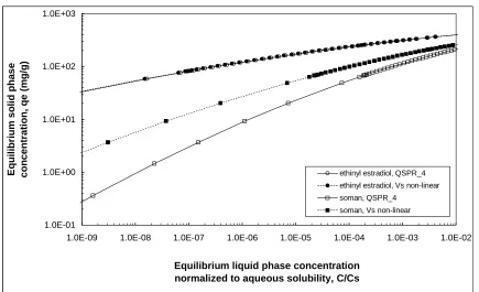
Additional predictions were made to compare the adsorption capacities of six

activated carbons with a wide range of physicochemical properties for the endocrine

disruptor ethinyl estradiol, which is relatively non-polar, and the nerve agent soman, which is

relatively polar. Among the six activated carbons, the activated carbon with the highest

oxygen content (Picazine, 15.9% oxygen) was predicted to have the lowest adsorption

capacities for ethinyl estradiol and soman at low C/Cs values. This result was particularly

interesting because the wood-based Picazine activated carbon had the largest BET surface

area and micropore volume of the tested activated carbons.

Overall, a new procedure was developed that permits the prediction of adsorption

isotherms from fundamental adsorbent and adsorbate properties. With respect to adsorbent

properties, the procedure requires the development of a reference curve from N2 and CO2

isotherm data and knowledge of the adsorbent’s oxygen and ash contents. With respect to

adsorbate properties, molecular descriptors are required that can be obtained quickly with

molecular modeling software packages. Once the affinity coefficient of a target contaminant

is calculated from the poly-parameter QSPR and the affinity coefficient of water is calculated

from the adsorbent’s oxygen content, a composite contaminant/water affinity coefficient can

be obtained for the adsorbate/adsorbent pair of interest. This composite contaminant/water

affinity coefficient can then be used to scale the reference curve such that the adsorption

isotherm for the desired adsorbate/adsorbent pair is obtained. To date, only a limited external

validation of the QSPRs developed in this study was conducted. To enhance the confidence

in the predictive powers of the developed QSPRs, a more comprehensive external validation

(4)

specific interactions between polar organic contaminants and oxygen-containing functional

(5)

PREDICTING THE ADSORPTION CAPACITY OF ACTIVATED

CARBON FOR ORGANIC CONTAMINANTS FROM FUNDAMENTAL

ADSORBENT AND ADSORBATE PROPERTIES

by

ISABELLA ANNA MEZZARI

A thesis submitted to the Graduate Faculty of North Carolina State University

in partial fulfillment of the requirements for the Degree of

Master of Science

CIVIL, CONSTRUCTION, AND ENVIRONMENTAL ENGINEERING

Raleigh

2006

APPROVED BY:

_______________________________

Dr. Francis L. de los Reyes III

________________________________

Dr. Morton Barlaz

________________________________

Dr. Detlef R.U. Knappe

(6)

BIOGRAPHY

Isabella Anna Mezzari was born in July, 1977 in Florianópolis, state of Santa

Catarina in Brazil. She graduated from the Federal University of Santa Catarina in December

1999, with a Bachelor of Science degree in Food Engineering. In July 2000, she obtained a

Bachelor of Science degree in Business Administration from Santa Catarina State University.

In 2002, she received a Master of Science degree in Chemical Engineering from the

Department of Chemical and Food Engineering at the Federal University of Santa Catarina,

where she worked as a research and teaching assistant in the Environmental and Energy

Laboratory under the sponsorship of the National Counsel of Technological and Scientific

Development (CNPq). In 2004, Isabella started studying at North Carolina State University

in the Water Resources and Environmental Engineering program towards a Master of

Science degree in Civil Engineering from the Department of Civil, Construction and

(7)

ACKNOWLEDGEMENTS

I would like to express my gratitude to my advisor, Dr. Detlef R. U. Knappe, for his

guidance and support throughout my M.S. studies. I extend my gratitude to Dr. Francis L. de

los Reyes III and Dr. Morton Barlaz for serving as members of my committee. I would also

like to thank the United States Environmental Protection Agency for sponsoring this

research.

I would like to thank my parents and my brother for their unconditional love and

support overseas. My special thanks goes to my sister, Dr. Melissa Paola Mezzari and my

brother in law, Dr. Márcio Luís Busi da Silva, whose knowledge in the environmental

engineering field has always inspired me and whose encouragement was essential for helping

me achieve my goals. I would like to express my deepest gratitude to Juan José Recalde for

(8)

LIST OF TABLES

Table 3.1 Activated Carbon Samples received from U.S. EPA...17

Table 3.2 Additional adsorbents used for model validation and isotherm predictions...18

Table 3.3 Freundlich isotherm constants for 62 neutral organic contaminants ...19

Table 3.4 Measured and accepted values of C, H and N for the NIST standard reference material. ...22

Table 3.5 Aqueous solubility data for chemicals that are liquids at 24°C...26

Table 3.6 Subcooled liquid solubility data for chemicals that are solids at 24°C ...27

Table 4.1 Physical adsorbent characteristics. ...36

Table 4.2 Chemical adsorbent characteristics...39

Table 4.3 Affinity coefficients for water (βw/benzene) ...41

Table 4.4 Total accessible pore volume of adsorbents. ...42

Table 4.5 Composite water/contaminant affinity coefficients, βlw,i/benzene, and contaminant affinity coefficients, βl,i/benzene, calculated from U.S. EPA isotherm data for 62 neutral organic contaminants. ...44

Table 4.6 One-parameter QSPR correlations...45

Table 4.7 Correlation Analysis Results ...49

Table 4.8 Poly-parameter QSPRs ...50

Table 4.9 Summary of statistical analyses ...53

(12)

LIST OF FIGURES

Figure 1.1 Flow chart outlining the modeling approach...3

Figure 2.1 Schematic model of an adsorbent pore showing the equipotential surfaces

corresponding to successively lower values of the adsorption potential with

increasing pore size (Manes, 1998). ...5

Figure 2.2 Characteristic curves of two substances on the same activated carbon. (Manes,

1998). ...7

Figure 3.1 Reference curve and aqueous-phase 1,1,2-Trichloroethane (TCA) adsorption

isotherm data. Adsorbent: F400 old...28

Figure 4.1 Micropore size distribution of adsorbents used for QSPR calibration. ...38

Figure 4.2 Micropore size distribution of adsorbents used for model validation and

isotherm predictions...38

Figure 4.3 Benzene reference curve. Adsorbent: F400(old)...43

Figure 4.4 Relationship between experimental βl,i/benzene values and βl,i/benzene values

calculated with the correlation obtained non-linearly with surface volume.

Straight line depicts 1:1 relationship...46

Figure 4.5 Scaled isotherm data for 46 neutral organic contaminants on F400(old).

Model: Vs non-linear. RMSE is for εscaled. ...47

Figure 4.6 Relationship between experimental βl,i/benzene values and βl,i/benzene values

calculated with the QSPR_4 model. Straight line depicts 1:1 relationship. ...51

Figure 4.7 Scaled isotherm data for 46 neutral organic contaminants on F400(old).

Model: QSPR_4. RMSE is for εscaled. ...51

Figure 4.8 Effect of molecular size on experimental and calculated values of βl,i/benzene.

Model: QSPR_4. ...55

Figure 4.9 Root mean square error associated with QSPR predictions of βl,i/benzene for

(13)

Figure 4.10 Root mean square errors associated with QSPR predictions of βl,i/benzene for

compounds in different chemical classes. (a) halogenated alkyl hydrocarbon,

monoaromatic hydrocarbon, monoaromatic halogenated; (b) triazine,

carbamate, chloroacetanilide, organophosphorus; (c) ketone, organochlorine,

urea, nitro compounds...58

Figure 4.11 Adsorption isotherm data and predicted adsorption isotherms for MTBE on

adsorbents F600, G219, OAW15 and Picazine. Adsorption isotherm data from

Li et al. (2002). ...61

Figure 4.12 Adsorption isotherm data and predicted adsorption isotherms for MTBE on

adsorbents CC-602 and UC-830. Adsorption isotherm data from Rossner

Campos (unpublished). ...61

Figure 4.13 Adsorption isotherm data and predicted adsorption isotherms for TCE on

adsorbents F400(old). Adsorption isotherm data from Speth (1990). ...63

Figure 4.14 Adsorption isotherm data and predicted adsorption isotherms for TCE on

adsorbents F600, G219, OAW15 and Picazine. Model: QSPR_4. Adsorption

isotherm data from Li et al. (2002). ...64

Figure 4.15 Adsorption isotherm data (pH 3.6) and predicted adsorption isotherms for

sulfamethoxazole (SMX) on adsorbents F600, CC-602, and UC-830. ...65

Figure 4.16 Adsorption isotherm predictions for selected chemical warfare agents.

Model: QSPR_4. Activated Carbon: F400(old). Isotherm prediction for VX

and nitrogen mustard are for the neutral form. ...68

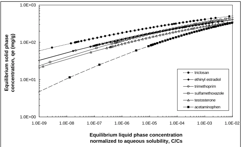
Figure 4.17 Adsorption isotherm predictions for selected pharmaceutically active

compounds and endocrine disruptors. Model: QSPR_4. Activated carbon:

F400(old). For all compounds, isotherm predictions are for the neutral form. ...68

Figure 4.18 Adsorption isotherm predictions for selected pesticides. Model: QSPR_4.

Activated carbon: F400(old). ...69

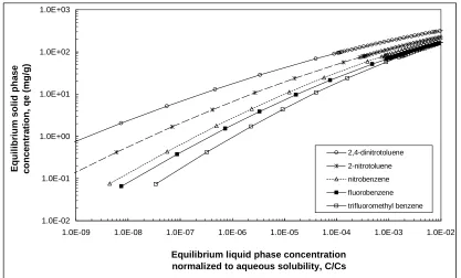
Figure 4.19 Adsorption isotherm predictions for monoaromatic compounds. Model:

(14)

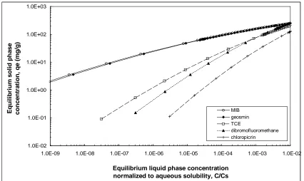
Figure 4.21 Adsorption isotherm predictions for taste and odor compounds and

halogenated aliphatic compounds. Model: QSPR_4. Activated carbon:

F400(old)...70

Figure 4.22 Adsorption isotherm predictions for ethinyl estradiol on 8 activated carbons.

Model: QSPR_4. ...74

Figure 4.23 Adsorption isotherm predictions for soman on 8 activated carbons. Model:

QSPR_4...74

Figure 4.24 Predicted adsorption isotherm of ethinyl estradiol (Cs, liquid = 401 mg/L) and

soman (Cs = 21,000 mg/L) on activated carbon F400(old) using one- and

(15)

1. INTRODUCTION AND OBJECTIVES

Activated carbon adsorption is a powerful technology for removing organic

contaminants from water. Information about adsorption isotherms is crucial for selecting the

most effective activated carbon for water treatment applications. Many activated carbons

with different physical and chemical characteristics are manufactured, and only few isotherm

data are available for the approximately 87,000 chemical substances and mixtures currently

in use. As a result, selecting the most cost-effective activated carbon for a given treatment

objective presents a challenge to water treatment professionals. In addition, collection of

adsorption isotherm data can be difficult because of a compound’s toxicity, analytical

challenges (instrument availability, cost), and time requirements to complete the

experiments. Therefore, the development of a model capable of predicting the adsorption

capacity of activated carbons from fundamental adsorbent and adsorbate properties would be

of great benefit to the water treatment industry.

The principal objectives of this research were (1) to identify a set of molecular

descriptors that define the affinity of organic contaminants for activated carbon and (2) to

incorporate the resulting quantitative structure-property relationship (QSPR) into the

Polanyi-Dubinin-Manes (PDM) model to predict single-solute adsorption isotherms for

currently regulated organic contaminants, organic compounds on the EPA Contaminant

Candidate List (CCL), emerging contaminants (e.g., endocrine disruptors, pharmaceutically

(16)

§ Characterize two GACs (Calgon F400, Norit 1240) that were used by the U.S.

EPA to collect single-solute isotherm data for currently regulated contaminants,

contaminants on the CCL, and contaminants of potential regulatory interest

(Speth and Miltner 1990, 1998; Speth unpublished data).

§ Calculate the affinity coefficient of water (βw/reference) for each adsorbent from the

adsorbent’s oxygen content.

§ Calculate the composite contaminant/water affinity coefficient (β1w,i/reference) of

each contaminant from single-solute isotherm data. From β1w,i/reference and

βw/reference, calculate contaminant affinity coefficients (β1,i/reference) of each

pollutant.

§ Calculate molecular descriptors for each contaminant using molecular

mechanics/dynamics and quantum mechanical algorithms.

§ Develop a QSPR that permits the prediction of β1,i/reference from suitable molecular

descriptors.

§ Predict single-solute adsorption isotherms of regulated organic contaminants

organic compounds on the EPA Contaminant Candidate List (CCL), emerging

contaminants (endocrine disruptors, pharmaceutically active compounds, personal

care products), and chemical agents (nerve agents, blister agents) on

well-characterized adsorbents with a wide range of physicochemical properties.

To effectively apply the PDM model for aqueous pollutants, coefficients describing

(17)

affinity coefficient of water was predicted from the adsorbent oxygen content using a

correlation developed by Li et al. (2005). Affinity coefficients of individual adsorbates were

calculated from isotherm data collected by the U.S. EPA for 62 neutral organic contaminants

on Calgon F400 and Norit 1240 activated carbons. Subsequently, molecular descriptors were

identified, from which affinity coefficients of individual adsorbates can be predicted.

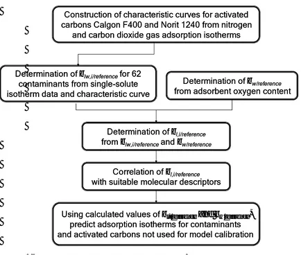
The overall modeling approach is summarized in Figure 1.1.

Figure 1.1 Flow chart outlining the modeling approach.

Determination of βlw,i/referencefor 62 contaminants from single-solute isotherm data and characteristic curve

Construction of characteristic curves for activated carbons Calgon F400 and Norit 1240 from nitrogen

and carbon dioxide gas adsorption isotherms

Determination of βw/reference from adsorbent oxygen content

Determination of βl,i/reference from βlw,i/referenceand βw/reference

Correlation of βl,i/reference with suitable molecular descriptors

Using calculated values of βl,i/referenceand βw/reference,

predict adsorption isotherms for contaminants and activated carbons not used for model calibration Determination of βlw,i/referencefor 62

contaminants from single-solute isotherm data and characteristic curve

Construction of characteristic curves for activated carbons Calgon F400 and Norit 1240 from nitrogen

and carbon dioxide gas adsorption isotherms

Determination of βw/reference from adsorbent oxygen content

Determination of βl,i/reference from βlw,i/referenceand βw/reference

Correlation of βl,i/reference with suitable molecular descriptors

Using calculated values of βl,i/referenceand βw/reference,

(18)

2. BACKGROUND

2.1. Polanyi-Dubinin-Manes Model

The Polanyi-Dubinin-Manes (PDM) model has its roots in the Polanyi Potential

Theory (Polanyi 1916, 1920, 1932), which was originally developed to describe the

adsorption of gases and vapors on activated carbon. The work of Polanyi was further

developed by Dubinin and co-workers into the Theory of Volume Filling of Micropores,

which included the derivation of the Dubinin-Radushkevich and Dubinin-Astakhov isotherm

equations (Dubinin 1960, 1966, 1972). In the 1970s, Manes and co-workers extended the

Polanyi modeling framework to describe the adsorption of aqueous organic contaminants on

activated carbon (Wohleber and Manes 1971, Manes 1998).

2.1.1. Adsorption of Gases/Vapors

Polanyi first postulated that adsorption on heterogeneous adsorbents, such as

activated carbon, occurs by a pore filling mechanism (Figure 2.1) and that the adsorbed

substance is present in a liquid or solid phase depending on the state of the pure compound at

the adsorption temperature. Heterogeneous adsorbents are characterized by pores of varying

size, and the highest adsorption energies are associated with the smallest pores that are

accessible to a given contaminant.

An essential parameter of the PDM model is the adsorption potential, ε1, defined as

the energy required to remove a molecule from its location in the adsorbent pore to a distance

outside the force field of the activated carbon. Because force fields of closely spaced pore

(19)

size; in other words, more energy is required to remove a chemical from smaller pores than

from larger pores.

Figure 2.1 Schematic model of an adsorbent pore showing the equipotential surfaces

corresponding to successively lower values of the adsorption potential with increasing pore size (Manes, 1998).

The adsorption potential for gases is described by Equation 1

    =

p p

RT sat

l ln

ε (1)

where ε1 is the adsorption potential (J/mol), R is the universal gas constant (8.314 J/molK), T

is the equilibrium temperature (K), Psat is the vapor pressure of the gas, and P is the

(20)

Polanyi (1916, 1920) further proposed that a temperature-invariant relationship exists

between the adsorbed volume of a given substance and the adsorption potential. Therefore, a

plot of adsorbed volume vs. adsorption potential at different temperatures is a unique curve

for a given substance, and this curve is known as the characteristic curve:

[ ]



  

 

    =

=

p p RT f f

V sat

l

adsorbed ε ln (2)

Polanyi (1916, 1920) assumed that, for a given activated carbon, all adsorbates

occupy a common limiting adsorption volume at zero adsorption potential, which is

represented by the maximum adsorption capacity, or total pore volume, of that adsorbent.

For gases and vapors, the adsorbed volume is calculated from the Equation 3:

  

 =

) ( 22414

1 3

gas cm mol V

V

Vadsorbed gas m (3)

where Vadsorbed is the adsorbed volume, cm3 (of solid)/100g; Vgas is the measured volume of

adsorbed gas, cm3 (gas at STP)/100g; and Vm is the molar volume of the liquid or solid

adsorbate at the temperature of the experiment, cm3/mol.

The characteristic curves of different substances on a given activated carbon tend to

have the same shape, but they differ by a constant scale factor in the adsorption potential

abscissa (Figure 2.2), and this scale factor is called the affinity coefficient, βl,i/reference.

Consequently, at a given Vadsorbed, the affinity coefficient of a contaminant relative to a

reference compound can be determined from the ratio of the adsorption potentials of the two

compounds (Equation 4):

reference l

i l reference

i l

, , /

, _ε

ε

(21)

where ε1,reference is the adsorption potential of a reference vapor; ε1,iis the adsorption potential

of the target compound; and βl,i/reference is the affinity coefficient of the target compound

relative to the reference compound. Often benzene is taken as the reference compound, then,

βl,i/reference = 1 for benzene, and the benzene adsorption potential curve is the reference curve.

Figure 2.2 Characteristic curves of two substances on the same activated carbon. (Manes, 1998).

2.1.2. Adsorption from the Aqueous Phase

For the adsorption of a partially miscible solute from aqueous solution, Polanyi

(1916) showed that the adsorption potential is calculated from:

      =

c c

RT S

i

lw, ln

(22)

where εlw,i is the adsorption potential of the aqueous target compound, and cS and c are the

saturation and bulk concentrations of the aqueous target compound, respectively.

The adsorbed volume of aqueous solutes can be obtained from Equation 6.

MW mol qV

Vadsorbed = m (6)

where Vadsorbed is the adsorbed volume, cm3 (liquid or solid)/100g; q is the mass of pollutant

adsorbed per mass of adsorbent, g/100g; Vm is the molar volume of the adsorbate at the

temperature of the experiment, cm3 (liquid or solid)/mol; and MW is the molecular weight of

the adsorbate, g.

The adsorption potential of an aqueous substance, as calculated from equation 6, is

influenced by the presence of water and represents the difference between the adsorption

potential of the pure compound and the adsorption potential of an equal volume of water that

needs to be displaced by the adsorbing compound (Manes, 1998). That is,

    − = w m w i, l i, lw V V ε ε ε (7)

where εw is the adsorption potential for water, and Vm and Vw are the molar volumes

(cm3/mol) of the adsorbate and water, respectively.

Returning to the affinity coefficient concept, Equation 4 can be adapted for aqueous

pollutants as follows:

(

)

₍

₎

w m ref w ref i l ref l w m w i l ref l i lw ref i

lw V V

V V / / / / , , , , , / , β β ε ε ε ε ε

(23)

where βlw,i/ref is a composite affinity coefficient that incorporates both the affinity coefficients

of the target adsorbate, βl,i/ref, and water, βw/ref, relative to the reference compound, benzene.

2.2. Determination of Affinity Coefficients

2.2.1. Affinity Coefficient of Water

The affinity coefficient of water can be determined directly from water adsorption

isotherm data or enthalpy of immersion data (Wood, 2001), or indirectly from adsorption

isotherm data of aqueous organic contaminants (e.g., Wohleber and Manes 1971, Li et al.

2005).

Wood (2001) reported values of the affinity coefficient of water relative to benzene,

obtained from water adsorption isotherms experiments performed by Stoeckli et al. (1994),

Matsumura et al. (1985), Barton et al. (1987) and Tamon et al. (1996) for several activated

carbons. The results showed that a single value cannot be assumed for βw/ref, since a wide

range of values for this parameter was obtained for carbons with different surface properties.

In addition, for a series of Calgon BPL activated carbons that were oxidized to different

degrees, the authors obtained a range of 0.11-0.19 for βw/benzene for high water pressures.

Stoeckli and Lavanchy (2000), by correlating calculated and experimental enthalpies

of immersion into water, showed that adsorption of water is governed by the oxygen content

of the carbon. They reported an extrapolated value of 0.052 for the water affinity coefficient

(24)

Slasi et al. (2003) reported a range of βw/benzene varying between 0.065 and 0.150,

depending on the surface chemistry of the adsorbent.

Li et al. (2005) obtained βlw,i/benzene from aqueous TCE and MTBE adsorption

isotherm data that were collected on twelve activated carbons with a wide range of oxygen

contents. Using equation 8 and βl,TCE/benzene and βl,MTBE/benzene values that were predicted from

parachor ratios, the affinity coefficient of water, βw/benzene was computed for each adsorbent.

A correlation between βw/benzene and the adsorbents’ oxygen contents resulted in the

expression:

0711 . 0 00353 . 0

/benzene = x+ w

β (r2 = 0.950) (9)

where x is the adsorbent oxygen content, in mmolO/g [daf].

2.2.2. Affinity Coefficients of Organic Compounds

Many researchers have attempted to identify molecular descriptors from which the

affinity coefficient βl,i/benzene can be calculated. Both one-parameter (Wood 2001) and

poly-parameter relationships (e.g. Wu et al., 2002) have been proposed for the calculation of

βl,i/benzene.

2.2.2.1. One-parameter relationships

Among the one-parameter relationships, βl,i/benzene is most commonly calculated from

molar volume (Vm), molar polarizability (P), or parachor (Ω) of the adsorbate. These

(25)

(ACDLabs, Toronto, ON) that calculates liquid molar volume, polarizability and parachor

from additive atomic increments.

Molar volume, Vm (cm3/mol) is described by equation 10:

ρ MW

V_m = (10)

where MW is the molecular weight (g/mol) and ρ is the density of the substance (g/cm3).

Molar polarizability (P, cm3/mol), which is also known as molar refractivity (e.g. in

ChemSketch), is defined as the dipole moment induced by an electric field. It is proportional

to electric dipole polarizability, which is a measure of the ease with which the electrons of a

molecule are distorted (Arnett et al., 1988). P can be calculated by the Lorenz-Lorentz

Equation (Todeschini and Consonni, 2000):

L D

D MW

n n P

ρ

  

 + − =

2 1

2 2

(11)

where nD (unitless), MW (g/mol) and ρL (g/cm3) are the refractive index, the molecular

weight, and the liquid density of the adsorbate, respectively.

Molar polarizability can also be computed from the polarizability of a molecule, α

(Bortolini et al., 1994):

α π. . 3 4

N

P= (12)

where N is the Avogadro’s number and α is the polarizability of the molecule (cm3) as calculated by ChemSketch.

(26)

4 / 1

γ ρ 

   =

Ω MW (13)

where γ is the surface tension of the substance.

Wood (1992) provided a database of 123 values of βl,i/reference2 compiled and

calculated from 14 published and unpublished sources. These values were for gas and vapor

adsorbates including nonpolar, polar and hydrogen-bonding compounds. Using the

Dubinin/Radushkevich (DR) equation, Wood (1992) successfully merged adsorption

isotherms for widely different compounds from many experimental sources when affinity

coefficients were calculated from molar polarizability.

In a subsequent study, Wood (2001) developed direct correlations between

experimental affinity coefficients and the molecular descriptors parachor, molar

polarizability, molar volume, and critical temperature. Power functions of the form β = aXm

were developed from each parameter using benzene as the reference compound. The best

results were obtained with polarizability, parachor, and molar volume with the correlations

β = 0.0862(P)0.75, β = 0.00827(Ω)0.90, and β = 0.0176(Vm)0.90, respectively. He concluded that

any of these correlations can be used to predict βl,i/reference. However, he pointed out some

advantages of using molar polarizability as a correlating parameter, such as: the ease of its

calculation; the temperature-invariant characteristic of polarizability; the more fundamental

theoretical relation to adsorption potential than molar volume or parachor; and the fact that

electronic polarizations include electrostatic as well as dispersion forces.

In a study by Reucroft et al. (1971), adsorption-desorption isotherm data were

(27)

(nonpolar, weakly polar and polar compounds) and took a representative organic vapor from

each group as the reference compound for each group, arguing that the best agreement

between the theoretical affinity coefficient and the experimental one is obtained when a

reference compound in each of the groups is used to calculate βl,i/reference. After relating the

affinity coefficients to molar polarizability and parachor, the results showed that the

percentage deviation between the values was greater when relating βl,i/reference with parachor

than with molar polarizability, especially in the case of polar compounds.

2.2.2.2. Poly-parameter Linear Relationships

It has always been assumed that βl,i/reference is proportional to one of the molecular

properties discussed in the previous section, even though each parameter accounts only for

non-specific van der Waals interactions. However, specific interactions (e.g.,

hydrogen-bonding, π-π electron donor-acceptor interactions) between an adsorbate and activated

carbon pore surfaces may also be important.

According to Goss and Schwarzenbach (2001), no single parameter is able to describe

appropriately all molecular interactions that determine the equilibrium partitioning of a given

compound between two phases. Therefore it is appropriate to select a group of molecular

descriptors that accounts for all of the forces governing physical adsorption.

One approach for predicting properties of chemicals is the development of

quantitative structure-property relationships (QSPRs). A QSPR is a mathematical

(28)

an equation that relates the property of interest, Y, with the descriptors chosen to be the most

important descriptors:

...

3 3 2 2 1

1 + + +

=

∑

a X a X a X a X

Y i

i

i (14)

where, Xi, represents a set of chosen descriptors and ai are the regression coefficients.

To describe molecular structure, a number of descriptors can be used in the QSPR

development, which can be classified as follows (Todeschini et al., 2000; Karelson, 2000):

• Quantum-chemical descriptors. These descriptors are obtained from

quantum-mechanical calculations, performed by means of algorithms, such as MOPAC,

GAUSSIAN98, GAMESS, METECC, AMPAC, and SPARTAN. Examples of

quantum-chemical descriptors include :

o Highest occupied molecular orbital energy (εHOMO) – According to Todeschini, et al. (2000), this property represents the highest energy level containing electrons in

the molecule, reflecting a measure of its nucleophilicity. Molecules with high

HOMO energy values are more reactive, because they can donate their electrons

more easily compared to molecules with low HOMO energy values.

o Lowest unoccupied molecular orbital energy (εLUMO) – This property represents

the lowest energy level that does not contain electrons in the molecule. According

to Todeschini, et al. (2000), molecules with low LUMO energy values are better

able to accept electrons than molecules with high LUMO energy values. It is a

measure of the electrophilicity of a molecule.

• Constitutional descriptors reflect the molecular composition of a compound without any

(29)

used descriptors, e.g., number of atoms, number of bonds, molecular weight, etc.

(Todeschini et al., 2000).

• Geometrical descriptors are derived from the three-dimensional structure of the

molecule. Examples of geometrical descriptors include: molecular surface area,

molecular volume, and solvent-accessible molecular surface area (Todeschini et al.,

2000; Karelson, 2000).

• Electrostatic descriptors encode information about the charge distribution in molecules.

Examples of electrostatic descriptors include dipole moment, molecular polarizability,

electrostatic hydrogen-bond basicity (defined as the magnitude of the charge on the most

negatively charged solute atom), and electrostatic hydrogen-bond acidity (defined as the

charge on the most positively charged solute hydrogen) (Todeschini et al., 2000).

• Substructure descriptors represent counts of predefined structural features in the

molecules. These descriptors form the basis group contribution approaches.

Once the descriptors are calculated, simple linear regression, multiple linear

regression, stepwise regression, or neural networks are used to correlate the descriptors with

the chemical property. A statistical test is applied to the resulting equations to determine if

the equations are significant. Due to the nature of statistics, the equations that give the best fit

do not necessarily have physical meaning. However, a QSPR may be constructed in which

the descriptors are physically meaningful (Magnuson and Speth, 2005).

Few QSPRs have been developed for the prediction of affinity. Qi et al. (2000)

(30)

first order valence molecular connectivity index, χv. This parameter is a molecular structure

descriptor originally developed by Kier and Hall (1986) which can be calculated directly

from the molecular structure of a chemical by an algorithm proposed by Prakash et al.

(1994). Equation 15 provides the correlation developed by Qi et al. (2000):

βl,i/ref = 0.3690 χv + 0.2729, (r2 = 0.967) (15)

where βl,i/reference is the affinity coefficient of an adsorbate relative to benzene, and χv is the modified first order valence molecular connectivity index of the adsorbate.

Wu et al. (2002) examined the relationship between affinity coefficients and

physico-chemical properties of adsorbates through the use of QSPR, or, in the teriminology of the

authors, Quantitative-Structure-Affinity Relationship (QSAfR). They related 40 common

organic chemicals, including hydrocarbons, halogenated hydrocarbons, monofunctional

amines, carbonyl compounds, alcohols, ethers, and a few other compound classes, to 45

physico-chemical parameters. Five of the 45 parameters were taken as principal components

of the relationship, accounting for 78.8% of the total variation in the data. Furthermore, Wu

et al. (2002) found that 3 descriptors were sufficient to account for 98.9% of the variance in

βl,i/reference . These parameters were molecular volume (volume), molecular weight (Mw) and

van der Waals interaction energy with a model graphite surface (Einter):

βl,i/ref = -0.0731 + 0.00182 Mw + 0.00418 volume – 0.0132 Einter (16)

With the proposed model, the root mean square error (RMSE) of βl,i/ref predictions for

40 contaminants was 0.090, compared to RMSE values of 0.141, 0.141 and 0.180 that were

obtained with one-parameter relationships based on based on parachor, molar polarizability

(31)

3. MATERIALS AND METHODS

3.1. Activated Carbons

Three activated carbon samples (Table 3.1) were obtained from the United States

Environmental Protection Agency (U.S. EPA). After their receipt at NC State University,

activated carbon samples were stored in a desiccator at room temperature. At NC State

University, physical and chemical characteristics of the activated carbon samples shown in

Table 3.1 were determined as described below. Activated carbon samples F400(old) and

F400(new) were the same product but taken from different lots; therefore, they were treated

as two individual activated carbon samples.

Table 3.1 Activated Carbon Samples received from U.S. EPA

Carbon Lot Mesh Date

1 Calgon F400(old) - 100 x 200 1980s

2 Calgon F400(new) w v 295-378 100 x 200 1989

3 Norit 1240 GAC 80222-7 100 x 200 1998

To verify the QSPRs developed in this study, adsorption isotherm predictions were

compared with adsorption isotherm data collected with F400(old) as well as with additional

adsorbents that were not part of the model calibration (Table 3.2). In addition, adsorption

isotherms for the compound classes shown in section 3.7 were predicted for the activated

carbons listed in Tables 3.1 and 3.2.

(32)

Table 3.2 Additional adsorbents used for model validation and isotherm predictions

Adsorbents Base Material

OAW15 thermally activated phenolic resin-based activated carbon fiber

(Nippon Kynol); acid–washed and subsequently oxidized with H2O2 (Li et al. 2002).

G219 thermally activated coconut shell-based GAC (PicaUSA,

Columbus,OH).

F600 thermally activated bituminous coal-based GAC (Calgon Carbon

Corporation, Pittsburgh, PA)

CC-602

(current designation: AquaCarb 1230C)

thermally activated coconut shell-based GAC (US Filter Westates Carbon, Conroe, TX)

UC-830 thermally activated coal-based GAC (US Filter Westates Carbon,

Conroe, TX)

Picazine chemically activated wood-based GAC (PicaUSA, Columbus,OH).

Norit HD4000 thermally activated lignite-based GAC (Norit Americas, Inc.)

The seven adsorbents listed in Tables 3.2 were physically and chemically

characterized following the procedures described in Section 3.3. Furthermore, the

characteristic curve and values of βw/benzene were obtained for each adsorbent as described in

Section 3.4.

3.2. Adsorption Isotherm Data

Adsorption isotherm data were obtained from the U.S. EPA for 62 neutral

contaminants. Isotherm data were collected with the three activated carbons shown in Table

3.1. Table 3.3 summarizes the Freundlich isotherm constants and their 95% confidence

intervals for each adsorbate-adsorbent pair. Data for each adsorption isotherm can be found

(33)

Table 3.3 Freundlich isotherm constants for 62 neutral organic contaminants

CAS # K

(µg/g)*(L/µg)1/n

1 toluene 108-88-3 5021 0.427 3650 to 6907 0.315 to 0.539

2 1,1-dichloroethane 75-34-3 65 0.705 52 to 80 0.660 to 0.751

3 1,1-dichloroethene 75-35-4 470 0.515 384 to 576 0.465 to 0.566

4 1,2-dichloroethane 107-06-2 129 0.533 82 to 204 0.445 to 0.621

5 1,2-dichloropropane 78-87-5 313 0.597 248 to 394 0.525 to 0.669

6 1,3-dichloropropane 142-28-9 897 0.497 724 to 1112 0.456 to 0.538

7 1,1,1-trichloroethane 71-55-6 335 0.531 219 to 513 0.443 to 0.620

8 1,2,3-trichloropropane 96-18-4 1080 0.613 825 to 1414 0.550 to 0.676

9 1,1,1,2-tetrachloroethane 630-20-6 1066 0.604 749 to 1518 0.521 to 0.686

10 1,1,2-trichloroethane 79-00-5 365 0.652 183 to 727 0.507 to 0.798

11 aldicarb 116-06-3 8267 0.402 6816 to 10027 0.338 to 0.466

12 atrazine 1912-24-9 38703 0.291 27427 to 54615 0.215 to 0.367

13 bromodichloromethane 75-27-4 241 0.655 222 to 263 0.635 to 0.675

14 benzene 71-43-2 1255 0.533 1149 to 1370 0.508 to 0.558

15 bromoform 75-25-2 929 0.665 706 to 1223 0.572 to 0.759

16 bromobenzene 108-86-1 17206 0.364 13486 to 21953 0.323 to 0.405

17 chlorobenzene 108-90-7 9167 0.348 7171 to 11718 0.298 to 0.397

18 chloroform 67-66-3 93 0.669 56 to 152 0.551 to 0.788

19 carbon tetrachloride 56-23-5 387 0.594 268 to 558 0.511 to 0.676

20 dibromochloromethane 124-48-1 585 0.636 529 to 647 0.604 to 0.668

21 dibromomethane 74-95-3 72 0.701 56 to 92 0.652 to 0.749

22 cis-1,2-dichloroethylene 156-59-2 202 0.587 172 to 238 0.549 to 0.625

23 1,2-dibromoethane 106-93-4 888 0.471 764 to 1032 0.421 to 0.520

24 ethyl benzene 100-41-4 9268 0.415 8621 to 9964 0.401 to 0.430

25 hexachlorocyclopentadiene 77-47-4 42964 0.504 27363 to 67460 0.365 to 0.643

26 lindane 58-89-9 15038 0.433 12222 to 18504 0.367 to 0.499

27 methylene chloride 75-09-2 6 0.801 4 to 9 0.717 to 0.886

28 metolachlor 51218-45-2 98195 0.125 80245 to 120161 0.092 to 0.158

29 metribuzin 21087-64-9 48693 0.193 40513 to 58526 0.165 to 0.221

30 o-dichlorobenzene 95-50-1 19258 0.378 13884 to 26713 0.312 to 0.444

31 tetrachloroethene 127-18-4 4054 0.516 3521 to 4669 0.478 to 0.554

32 p-dichlorobenzene 106-46-7 4969 0.691 3316 to 7447 0.570 to 0.812

33 p-xylene 106-42-3 12574 0.418 10987 to 14390 0.356 to 0.480

34 simazine 122-34-9 31346 0.227 25531 to 38486 0.144 to 0.310

35 styrene 100-42-5 12158 0.479 9359 to 15795 0.412 to 0.547

36 1,1-dichloropropene 563-58-6 2670 0.374 1621 to 4399 0.277 to 0.472

37 cyanazine 21725-46-2 102312 0.126 70975 to 147486 0.071 to 0.181

38 carbofuran 1563-66-2 16384 0.408 10758 to 24951 0.254 to 0.563

39 dibromochloropropane 96-12-8 6910 0.501 6015 to 7939 0.430 to 0.571

40 tert butyl methyl ether 1634-04-4 218 0.479 67 to 710 0.265 to 0.693

41 isophorone 78-59-1 9750 0.271 6169 to 15409 0.148 to 0.395

42 trans-1,2-dichloroethene 156-60-5 618 0.452 478 to 799 0.393 to 0.511

43 1,3,5-trichlorobenzene 108-70-3 63825 0.324 49608 to 82116 0.266 to 0.382

44 alachlor 15972-60-8 81677 0.257 72709 to 91750 0.225 to 0.289

45 o-chlorotoluene 95-49-8 23200 0.378 18542 to 29029 0.335 to 0.421

46 2,4-dinitrotoluene 121-14-2 96084 0.157 78368 to 117806 0.121 to 0.192

47 1,3-dichlorbenzene 541-73-1 5907 0.630 4216 to 8276 0.521 to 0.739

48 methyl isobutyl ketone 108-10-1 8850 0.279 5934 to 13199 0.202 to 0.356

49 m-xylene 108-38-3 4933 0.614 3096 to 7857 0.488 to 0.739

50 1,2-diphenylhydrazine 122-66-7 150059 0.089 137068 to 164280 0.067 to 0.112

51 1,2,4-trimethylbenzene 95-63-6 47783 0.240 40873 to 55860 0.204 to 0.276

52 p-cymene 99-87-6 50898 0.228 40600 to 63808 0.174 to 0.283

53 diazinon 333-41-5 252068 0.040 201042 to 316044 0.003 to 0.076

54 disulfoton 298-04-4 195088 0.063 137364 to 277069 0.007 to 0.119

55 diuron 330-54-1 136691 0.139 114922 to 162584 0.104 to 0.173

56 EPTC 759-94-4 79510 0.158 71655 to 88225 0.139 to 0.177

57 fonofos 944-22-9 250580 0.065 204273 to 307385 0.026 to 0.104

58 linuron 330-55-2 154721 0.108 138343 to 173038 0.085 to 0.130

59 molinate 2212-67-1 53696 0.226 45587 to 63248 0.192 to 0.259

CARBON NORIT 1240 (100X200 mesh)

(µg/g)*(L/µg)1/n

CARBON F400(OLD) (100x200 mesh)

K

1/n 1/n

Freundlich constants 95 percent confidence interval

(34)

3.3. Activated Carbon Characterization

3.3.1. BET Surface Area

Brunauer, Emmet and Teller (BET) surface areas were obtained from nitrogen

adsorption isotherm data collected at 77K (Autosorb-1,Quantachrome Corporation, Boynton

Beach, FL). Prior to analysis, activated carbon samples (0.1 g) were dried overnight at 105°C

and subsequently outgassed at 150°C for 20 hours. For BET surface area determinations, N2

adsorption isotherm data were collected in the relative pressure range of 0.01 to 0.1. A glass

rod was used during the analysis to decrease the void volume of the cell.

3.3.2. Pore Size Distribution

To determine the pore size distribution of activated carbons, additional nitrogen

adsorption isotherm experiments were conducted in two separate phases:

§ Phase 1 (high pressure range): Prior to analysis, 0.04 g of an activated carbon

sample was dried overnight at 105°C and subsequently outgassed at 150°C for 20

hours. Adsorption isotherms were constructed with 83 data points in the relative

pressure range of 0.001 to 1. A glass rod was used to decrease the void volume of

the cell. The activated carbon sample mass in this experiment was adjusted such

that the BET surface area obtained with this experiment matched that obtained

from the experiment with a larger sample mass described in Section 3.3.1.

§ Phase 2 (low pressure range): Adsorption isotherms were constructed with 38 data

(35)

glass rod was used in this relative pressure range to permit more rapid system

equilibration.

Upon completion of phase 1 and 2 experiments, isotherm data from both phases were

combined to produce one isotherm. When needed, the carbon sample mass from phase 2 (low

pressure range) was adjusted such that the volume adsorbed in the relative pressure range of

0.001 to 0.005 matched that obtained in the same relative pressure range in phase 1 (high

pressure range). Phase 1 and 2 isotherm data were used in the construction of the

characteristic curves (see Section 3.4) and for the determination of pore size distributions.

Micropore volume, mesopore volume and pore size distribution were computed from

N2 adsorption data using the Density Functional Theory (DFT) with the Kernel file

N2_carb1.gai (PC software version 1.51, Quantachrome, Boynton Beach, FL). Mesopore

volume was also computed using the BJH Method, since this method captures the entire

mesopore range (20 to 500 Å) while the DFT method was only able to calculate a mesopore

volume for pores with widths in the range of 20 to 360 Å.

3.3.3. Elemental Analysis

C, H and N contents of the activated carbons were determined using a CHN

Elemental Analyzer (Perkin-Elmer Corp., Norwach, CT) in the Soil Science Department at

North Carolina State University. The accuracy of the CHN analyzer was checked with a

(36)

Table 3.4 Measured and accepted values of C, H and N for the NIST standard reference material.

%C %H %N

Measured values 77.03 4.88 1.52

Accepted values 77.45 + 0.25 5.11 + 0.12 1.54 + 0.06

Oxygen content was determined by Huffman Laboratories (Golden, CO) according to

ASTM D5622. Ash content was determined following ASTM D 2866.

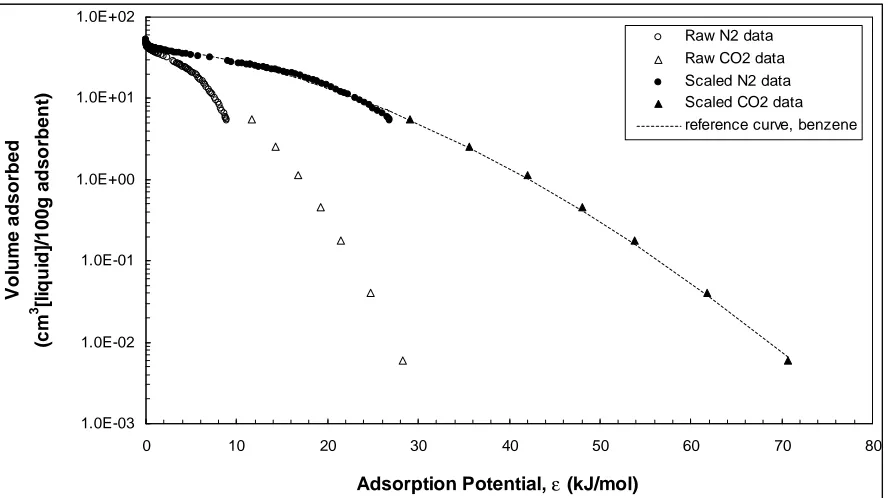
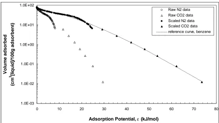
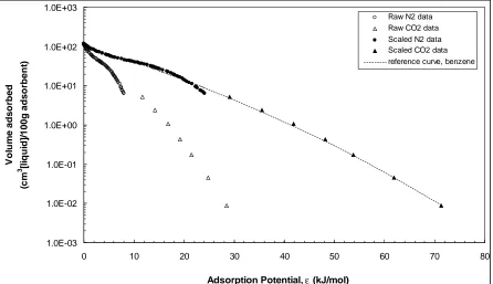
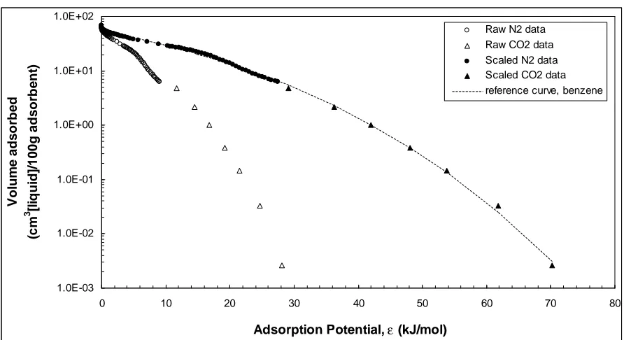
3.4. Reference Curve

Reference curves were constructed from N2 and CO2 adsorption isotherm data. Apart

from the phase 1 and 2 N2 adsorption experiments, CO2 adsorption experiments were

performed at 273.15K in the relative pressure range of 10-6 to 10-2 (the saturation pressure of

CO2 at 273.15 K is Po = 26142 mmHg).

From the N2 and CO2 isotherm data, adsorption potentials εl,i for the two gases were

computed using Equation 1. The adsorbed gas volume was transformed to adsorbed volume

using Equation 3, where molar volumes (Vm) of N2 and CO2 were calculated from their

respective densities in the adsorbed state (ρ = 0.808 g/cm3 for N2 at 77 K and ρ = 1.023

g/cm3 for CO2 at 273 K (Cazorla Amoros et al. 1996).

Using Equation 4, adsorption potentials of benzene (εbenzene), the reference compound,

were computed from the adsorption potentials of N2 and CO2 at any Vadsorbedwith the affinity

coefficients βl,N2/benzene = 0.33 and βl,CO2/benzene = 0.40 (Dubinin, 1966; Cazorla-Amoros, et al.

(37)

To construct the reference curve for each activated carbon, a third-order polynomial

fit (Manes 1998) was applied to relate Vadsorbed to εbenzene:

log (Vadsorbed)= a (εbenzene)3 + b (εbenzene)2 + c (εbenzene)+ d (17)

where, a ... d are regression coefficients.

3.4.1. Composite water/contaminant affinity coefficients

Adsorption potentials for each aqueous contaminant, εlw,i, were calculated from

equation 6, which requires equilibrium liquid phase concentration data (C) and the aqueous

solubility (Cs). Equilibrium liquid phase concentration data were obtained from adsorption

isotherm experiments conducted at the U.S. EPA.

In this study, aqueous solubilities were obtained from four sources: 1) the database

of Mackay et al. (1992), which recommends a most probable Cs value that was chosen from

experimentally determined solubility values obtained from different sources; 2) the database

of Horvath et al. (1999), which also provides a comprehensive review of published aqueous

solubility data and proposes a recommended Cs value for many contaminants; 3) the

PHYSPROP database (Syracuse Research Corporation, North Syracuse, NY); and 4) The

Pesticide Manual (Tomlin, 2003).

For solid contaminants at the temperature of the U.S. EPA isotherm experiments

(24°C), the subcooled liquid solubility, Cs.liquidwas used instead of Cs. Values of Cs,liquid were

taken from Mackay et al. (1992), who computed the subcooled liquid solubility following the

(38)

F C

C s

liquid ,

s = where _S

L

f f

F = (18)

where f Lis the fugacity of the liquid and f S is the fugacity of the solid.

The fugacity ratio is indicative of the Gibbs energy needed to convert solid i to liquid

i, at a particular temperature (Peters et al., 1997). F can be calculated using:

    

  

   



 ₋

  

 ∆−

=exp 1

T T RT

H

F m

m f

(19)

where ∆Hf is the enthalpy of fusion; R is the universal gas constant; Tm is the melting point

(K); and T is the system temperature (K).

The principal challenge with equation 19 is to find ∆Hf because not many enthalpy of

fusion data are available in the literature. For compounds for which ∆Hf data are not

available, an approximation can be used as proposed by Yallowsky (1979):

f m f

S T

H = ∆

∆ (20)

A common value for ∆Sf, the entropy of fusion at the melting temperature, is

assumed. Yallowsky (1979) demonstrated that for rigid molecules, the entropy of fusion is

roughly constant with a median value of 56 J/mol-K. Mackay et al. (1992) used this

approximation for compounds for which ∆Hf data were not available.

An illustrative example for the determination of the subcooled liquid solubility of

atrazine is shown below:

Input data:

(39)

Cs = 30 mg/L = 0.139095 mol/m3

Tm = 174oC = 447.15 K

              ₋     ∆−

=exp 1

T T R

S

F f m

            ₋       − = 1 15 . 298 15 . 447 / 314 . 8 / 56 exp molK J molK J F 0345 . 0 = F F C C s liquid , s = 0345 . 0 / 139095 . 0 3 , m mol C_s_liquid =

3 ,liquid =4.09103mol/m s

C

g/l 882.35294m ,liquid =

s C

Table 3.5 summarizes aqueous solubility data for chemicals that are liquids at 24°C,

the temperature at which isotherm experiments were conducted at the U.S. EPA, and Table

3.6 shows aqueous solubility and subcooled liquid solubility data for chemicals that are

(40)

Table 3.5 Aqueous solubility data for chemicals that are liquids at 24°C

Chemical Sample Cs (mg/L) Temperature Source

liquid chemicals at T = 24oC of Cs (

o C)

toluene 515 25 Mackay et al. (1992)

1,2-Dichloropropane 2800 25 Mackay et al. (1992)

1,2,3-trichloropropane 1896 25 Mackay et al. (1992)

bromodichloromethane 4500 25 Mackay et al. (1992)

benzene 1780 25 Mackay et al. (1992)

bromoform 3100 25 Mackay et al. (1992)

bromobenzene 410 25 Mackay et al. (1992)

chlorobenzene 484 25 Mackay et al. (1992)

chloroform 8200 25 Mackay et al. (1992)

carbon tetrachloride 800 25 Mackay et al. (1992)

dibromochloromethane 4000 25 Mackay et al. (1992)

dibromomethane 11442 25 Mackay et al. (1992)

ethyl benzene 152 25 Mackay et al. (1992)

methylene chloride 13200 25 Mackay et al. (1992)

metolachlor 430 25 Mackay et al. (1992)

o-dichlorobenzene 118 25 Mackay et al. (1992)

p-xylene 215 25 Mackay et al. (1992)

styrene 300 25 Mackay et al. (1992)

tert butyl methyl ether 42000 25 Mackay et al. (1992)

isophorone 12000 25 Mackay et al. (1992)

1,3-Dichlorobenzene 120 25 Mackay et al. (1992)

m-xylene 160 25 Mackay et al. (1992)

1,2,4-Trimethylbenzene 57 25 Mackay et al. (1992)

p-Cymene 34 25 Mackay et al. (1992)

Diazinon 60 25 Mackay et al. (1992)

Fonofos 16 25 Mackay et al. (1992)

Molinate 970 25 Mackay et al. (1992)

1,1-dichloroethane 5040 25 Horvath et al. (1999)

1,1-Dichloroethene 2420 25 Horvath et al. (1999)

1,2-Dichloroethane 8600 25 Horvath et al. (1999)

1,1,1-Trichloroethane 1290 25 Horvath et al. (1999)

1,1,1,2-Tetrachloroethane 1070 25 Horvath et al. (1999)

1,1,2-Trichloroethane 4590 25 Horvath et al. (1999)

cis-1,2-Dichloroethylene 6410 25 Horvath et al. (1999)

1,2-Dibromoethane 3910 25 Horvath et al. (1999)

tetrachloroethene 206 25 Horvath et al. (1999)

trans-1,2-dichloroethene 4520 25 Horvath et al. (1999)

1,3-Dichloropropane 2750 25 Yalkowsky and Dannenfelser (1992) (Syrres database)

methyl isobutyl ketone 19000 25 Yalkowsky and Dannenfelser (1992) (Syrres database)

hexachlorocyclopentadiene 1.8 25 Callahan et al. (1979) (Syrres database)

1,1-Dichloropropene 749 25 Meylan et al. (1996) (Syrres database)

dibromochloropropane 1230 20 Munnecke and Vangundy (1979) (Syrres database)

o-chlorotoluene 374 25 Valvani et al. (1981) (Syrres database)

EPTC 375 25 Tomlin (2001)

Acetochlor 223 25 Tomlin (2001)

(41)

Table 3.6 Subcooled liquid solubility data for chemicals that are solids at 24°C

Chemical Sample Cs (mg/L) Temperature Melting point Fugacity ratio at Cs,liquid Source

solid chemicals at T = 24oC of Cs (

o

C) MP (oC) temperature of Cs (mg/L)

metribuzin a 1050 20 126.2 0.102 10329.87 Tomlin (2001)

simazine a 6.2 22 226 0.011 581.39 USDA Pesticide Properties Database (Syrres database)

Diuron a 42 25 158 0.050 847.53 USDA Pesticide Properties Database (Syrres database)

Linuron a 75 25 93 0.215 348.52 USDA Pesticide Properties Database (Syrres database)

desethyl atrazine a 3200 22 133 0.087 36709.01 Mill and Thurman (1994A) (Syrres database)

RDX a 59.7 25 205.5 0.017 3523.04 Yalkowsky and Dannenfelser (1992) (Syrres database)

1,2-Diphenylhydrazine a

221 25 131 0.091 2423.22 Kuhner et al. (1995) (Syrres database)

aldicarb b 6000 25 99.5 0.185 32342.50 Mackay et al. (1992)

atrazine b 30 25 174 0.034 892.92 Mackay et al. (1992)

lindane b 7.3 25 112.5 0.136 53.52 Mackay et al. (1992)

cyanazine b 171 25 166.75 0.039 4339.82 Mackay et al. (1992)

carbofuran b 351 25 151 0.0567 6196.40 Mackay et al. (1992)

1,3,5-Trichlorobenzene b

5.3 25 64 0.41 12.92 Mackay et al. (1992)

alachlor b 240 25 41 0.695 345.58 Mackay et al. (1992)

2,4-Dinitrotoluene b 270 25 70 0.359 752.24 Mackay et al. (1992)

p-dichlorobenzene b 83 25 53.1 0.53 156.61 Mackay et al. (1992)

a

Fugacity ratio was computed from equations 19 and 20, while subcooled liquid solubility, Cs,liquid, was computed from equation 18.

b

(42)

The volume occupied by an adsorbed compound, Vadsorbed (cm3/100g carbon), was

computed using Equation 6, where q values (g/100g) were obtained from U.S. EPA isotherm

data, and values of molar volume and molecular weight were obtained with Chemsketch

(ACD Labs, Toronto, ON).

To determine the affinity coefficient of a given compound, a regression analysis was

conducted, in which the sum of squares of the difference between the scaled abscissa values

and the reference curve abscissa values at each experimental Vadsorbed were minimized as

shown in Figure 3.1.

1.0E-03 1.0E-02 1.0E-01 1.0E+00 1.0E+01 1.0E+02

0 10 20 30 40 50 60 70 80

Adsorption Potential, ε (kJ/mol)

V

o

lu

m

e

a

d

s

o

rb

e

d

(c

m

3 [l

iq

u

id

]

/1

0

g

a

d

s

o

rb

e

n

t)

reference curve

1,1,2-Trichloroethane (TCA)

At any V:

βlw = εTCA / εreference

Figure 3.1 Reference curve and aqueous-phase 1,1,2-Trichloroethane (TCA) adsorption

(43)

3.4.2. Affinity Coefficients of Water

The affinity coefficient of water, βw/benzene, was estimated for each activated carbon

from Equation 9, which relates βw/benzene to the adsorbent oxygen content (mmol O/g[daf]).

3.4.3. Affinity Coefficients of Contaminants

Once the affinity coefficient of water, βw/benzene, was determined, the affinity

coefficients of individual adsorbates, βl,i/benzene, were computed from the composite

water/contaminant affinity coefficient, βlw,i/benzene, using Equation 8. Molar volumes for each

adsorbate and water were both obtained from Chemsketch.

3.5. Development of Quantitative Structure-Property Relationships

One principal objective of this study was to develop quantitative structure-property

relationships (QSPRs) between affinity coefficients (βl,i/benzene) and molecular descriptors of

individual adsorbates. QSPRs were developed using βl,i/benzene values for the 62 neutral

organic contaminants for which isotherm data were available from the U.S. EPA (Table 3.2).

3.5.1. One-parameter QSPRs

To assess the feasibility of predicting βl,i/benzene values from a single molecular

descriptor, QSPRs were developed that relate βl,i/benzene with (1) molar volume (cm3/mol),

molar polarizability (cm3/mol), parachor (cm3/mol)(dyn/cm)0.25, solvent-accessible surface

(44)

Liquid molar volume at 20°C and parachor were calculated using Chemsketch v. 8.0

(ACD Labs, Toronto, ON). Molar polarizability values were obtained from Equation 12, and

polarizability values, α, were calculated using Chemsketch.

Solvent-accessible surface area, SASA, and surface volume, Vs, were computed with

CAChe WorkSystem Pro Version 6.1.8 (Fujitsu Limited). The solvent accessible surface of a

molecule is defined as the van der Waals envelope of the molecule expanded by the radius of

the solvent sphere about each atom center (Lee and Richards, 1971). The surface volume is

the volume enclosed by the molecular surface (Lee et al., 2003).

Appendix B summarizes the values of the five parameters for each of the 62

contaminants.

3.5.2. Poly-parameter QSPRs

For the development of poly-parameter QSPRs, ten molecular descriptors were

calculated for each adsorbate using CAChe. A criterion for their selection was that the

correlation coefficient between any two molecular descriptors should be between -0.85 and

0.85. Molecular descriptors were also scaled before QSPR development to assure that they

had similar statistical weight. Values of the ten molecular descriptors for each contaminant

can be found in Appendix C.

To obtain molecular descriptors, all molecules were initially built in the

ProjectLeaderTM table using the CAChe Editor (Fujitsu Limited). Subsequently, the

Predicting the Adsorption Capacity of Activated Carbon for Organic Contaminants from Fundamental Adsorbent and Adsorbate Properties

ABSTRACT

PREDICTING THE ADSORPTION CAPACITY OF ACTIVATED

CARBON FOR ORGANIC CONTAMINANTS FROM FUNDAMENTAL

ADSORBENT AND ADSORBATE PROPERTIES

by

ISABELLA ANNA MEZZARI

CIVIL, CONSTRUCTION, AND ENVIRONMENTAL ENGINEERING

APPROVED BY:

BIOGRAPHY

ACKNOWLEDGEMENTS

TABLE OF CONTENTS

LIST OF TABLES

LIST OF FIGURES

[ ]

(

)

(

)

∑

₍

₎