Bayesian Model Selection for Genome-Wide Epistatic Quantitative Trait Loci Analysis

©

DOI: 10.1534/genetics.104.040386

Bayesian Model Selection for Genome-Wide Epistatic Quantitative

Trait Loci Analysis

Nengjun Yi,*

,†,1

_{Brian S. Yandell,}

‡

_{Gary A. Churchill,}

§

_{David B. Allison,*}

,†

Eugene J. Eisen** and Daniel Pomp

††

*Department of Biostatistics, Section on Statistical Genetics,†_{Clinical Nutrition Research Center, University of Alabama, Birmingham,} Alabama 35294,‡_{Departments of Statistics and Horticulture, University of Wisconsin, Madison, Wisconsin 53706,}

§_{The Jackson Laboratory, Bar Harbor, Maine 04609,**Department of Animal Science, North Carolina} State University, Raleigh, North Carolina 27695 and††_{Department of Animal Science,}

University of Nebraska, Lincoln, Nebraska 68583 Manuscript received December 29, 2004

Accepted for publication April 4, 2005

ABSTRACT

The problem of identifying complex epistatic quantitative trait loci (QTL) across the entire genome continues to be a formidable challenge for geneticists. The complexity of genome-wide epistatic analysis results mainly from the number of QTL being unknown and the number of possible epistatic effects being huge. In this article, we use a composite model space approach to develop a Bayesian model selection framework for identifying epistatic QTL for complex traits in experimental crosses from two inbred lines. By placing a liberal constraint on the upper bound of the number of detectable QTL we restrict attention to models of fixed dimension, greatly simplifying calculations. Indicators specify which main and epistatic effects of putative QTL are included. We detail how to use prior knowledge to bound the number of detectable QTL and to specify prior distributions for indicators of genetic effects. We develop a computa-tionally efficient Markov chain Monte Carlo (MCMC) algorithm using the Gibbs sampler and Metropolis-Hastings algorithm to explore the posterior distribution. We illustrate the proposed method by detecting new epistatic QTL for obesity in a backcross of CAST/Ei mice onto M16i.

M

ANY complex human diseases and traits of bio- tive corrections for multiple testing. Non-Bayesian model

logical and/or economic importance are deter- selection methods combine simultaneous search with a

mined by multiple genetic and environmental influ- sequential procedure such as forward or stepwise

selec-ences (Lynch and Walsh 1998). Mounting evidence tion and apply criteria such asP-values or modified

Baye-suggests that interactions among genes (epistasis) play sian information criterion (BIC) to identify well-fitting

an important role in the genetic control and evolu- multiple-QTL models (Kaoet al.1999;Carlborget al.

tion of complex traits (Cheverud2000;Carlborgand 2000;Reifsnyderet al.2000;Bogdanet al.2004). These

Haley2004). Mapping quantitative trait loci (QTL) is methods, although appealing in their simplicity and

pop-a process of inferring the number of QTL, their geno- ularity, have several drawbacks, including: (1) the

uncer-mic positions, and genetic effects given observed pheno- tainty about the model itself is ignored in the final

in-type and marker genoin-type data. From a statistical per- _{ference, (2) they involve a complex sequential testing}

spective, two key problems in QTL mapping are model _{strategy that includes a dynamically changing null}

hy-search and selection (e.g., Broman and Speed 2002; _{pothesis, and (3) the selection procedure is heavily}

in-Sillanpa¨a¨andCorander2002;Yi 2004). Traditional _{fluenced by the quantity of data (Rafteryet al. 1997;}

QTL mapping methods utilize a statistical model, which _{George 2000;Gelmanet al.2004;KadaneandLazar}

estimates the effects of only one QTL whose putative _2004).

position is scanned across the genome (e.g.,Landerand _{Bayesian model selection methods provide a}

power-Botstein 1989; Jansen and Stam 1994; Zeng1994). _{ful and conceptually simple approach to mapping}

multi-Extensions of this approach can allow for main and epi- _{ple QTL (Satagopanet al.1996;Hoeschele2001;Sen}

static effects at two or perhaps a few QTL at a time and _{and Churchill 2001). The Bayesian approach}

pro-employ a multidimensional scan to detect QTL. How- _{ceeds by setting up a likelihood function for the}

pheno-ever, such an approach neglects potential confound- _{type and assigning prior distributions to all unknowns}

ing effects from additional QTL and requires prohibi- _{in the problem. These induce a posterior distribution}

on the unknown quantities that contains all of the avail-able information for inference of the genetic

architec-1_{Corresponding author:Department of Biostatistics, University of}

Ala-ture of the trait. Bayesian mapping methods can treat

bama, Ryals Public Health Bldg., 1665 University Blvd., Birmingham,

AL 35294-0022. E-mail: [email protected] the unknown number of QTL as a random variable,

A BAYESIAN MODEL SELECTION FRAMEWORK

which has several advantages but results in the

complica-FOR QTL MAPPING

tion of varying the dimension of the model space. The

reversible jump Markov chain Monte Carlo (MCMC) _{We consider experimental crosses derived from two}

algorithm, introduced byGreen(1995), offers a power- _{inbred lines. In QTL studies, the observed data consist}

ful and general approach to exploring posterior distri- _{of phenotypic trait values,y, and marker genotypes,m,}

butions in this setting. However, the ability to “move” _{for individuals in a mapping population. We assume that}

between models of different dimension requires a care- _{markers are organized into a linkage map and restrict}

ful construction of proposal distributions. Despite the _{attention to models with, at most, pairwise interactions.}

challenges of implementation of reversible jump algo- _{We partition the entire genome into H loci, ␨ ⫽ {␨1,}

rithms, effective approaches for mapping multiple non- _{. . . , ␨H}, and assume that the possible QTL occur at}

interacting QTL have been developed (Satagopanand _{these fixed positions. This introduces only a minor bias}

Yandell1996;Heath1997;Thomaset al.1997;Uimari in estimating the position of QTL whenHis large. When

andHoeschele1997;Sillanpa¨a¨andArjas1998;Ste- the markers are densely and regularly spaced, we set␨

phensandFisch1998;YiandXu2000;Gaffney2001). _{to the marker positions; otherwise,␨includes not only}

Bayesian model selection methods employing the re- _{the marker positions but also points between markers.}

versible jump MCMC algorithm have been proposed to _{In general, the genotypes,g, at loci␨are unobservable}

map epistatic QTL in inbred line crosses and outbred pop- _{except at completely informative markers, but their}

ulations (YiandXu2002;Yiet al.2003, 2004a,b;Narita _{probability distribution, p(g|␨,m), can be inferred from}

andSasaki2004). However, the complexity of the reversi- _{the observed marker data using the multipoint method}

ble jump steps increases computational demand and may _{(JiangandZeng1997). This probability distribution is}

prohibit improvements of the algorithms. _{used as the prior distribution of QTL genotypes in our}

Recently, Yi (2004) proposed a unified Bayesian _{Bayesian framework.}

model selection framework to identify multiple nonepi- _{The problem of inferring the number and locations}

static QTL for complex traits in experimental designs, _{of multiple QTL is equivalent to the problem of}

select-based upon a composite space representation of the _{ing a subset of␨that fully explains the phenotypic}

varia-problem. The composite space approach, which is a _{tion. Although a complex trait may be influenced by}

modification of the product space concept developed _{multitudes of loci, our emphasis is on a set of at most}

by Carlin and Chib (1995), provides an interesting _{LQTL with detectable effects. TypicallyLwill be much}

viewpoint on a wide variety of model selection prob- _{smaller thanH. Let ␭ ⫽ {␭1, . . . ,␭L} (僆{␨1, . . . ,␨H})}

lems (Godsill2001). The key feature of the composite _{be the current positions ofLputative QTL. Each locus}

model space is that the dimension remains fixed, _{may affect the trait through its marginal (main) effects}

allowing for MCMC simulation to be performed on a _{and/or interactions with other loci (epistasis). The}

phe-space of fixed dimension, thus avoiding the complexi- _{notype distribution is assumed to follow a linear model,}

ties of reversible jump. InYi(2004), the varying

dimen-y⫽␮⫹X␤⫹ e, (1)

sional space is augmented to a fixed dimensional space

(the composite model space) by placing an upper bound _{where ␮ is the overall mean, ␤ denotes the vector of}

on the number of detectable QTL. In the composite _{all possible main effects and pairwise interactions ofL}

model space, latent binary variables indicate whether _{potential QTL ,Xis the design matrix, andeis the}

vec-each putative QTL has a nonzero effect. The result- tor of independent normal errors with mean zero and

ing hierarchical model can vastly simplify the MCMC variance␴2_{. The number of genetic effects depends on}

search strategy. the experimental design, and the design matrix X is

In this work we extend the composite model space determined from those genotypesgat the current loci

approach to include epistatic effects. We develop a frame- ␭by using a particular genetic model (seeappendix a

work of Bayesian model selection for mapping epistatic for details of the Cockerham genetic model used here).

QTL in experimental crosses from two inbred lines. We There is prior uncertainty about which genetic effects

show how to incorporate prior knowledge to select an should be included in the model. As in Bayesian

vari-upper bound on the number of detectable QTL and able selection for linear regression (e.g., George and

prior distributions for indicator variables of genetic ef- McCulloch 1997;Kuo andMallick 1998; Chipman

fects and other parameters. A computationally efficient et al. 2001), we introduce a binary variable␥ for each

MCMC algorithm using a Gibbs sampler or Metropolis- effect, indicating that the corresponding effect is

in-Hastings (M-H) algorithm is developed to explore the cluded (␥ ⫽ 1) or excluded (␥ ⫽ 0) from a model.

posterior distribution on the parameters. The proposed Letting⌫⫽diag(␥), the model becomes

algorithm is easy to implement and allows more

com-y⫽␮⫹X⌫␤⫹e. (2)

plete and rapid exploration of the model space. We first

describe the implementation of this algorithm and then This linear model defines the likelihood,p(y|␥,X,␪),

illustrate the method by analyzing a mouse backcross with␪⫽(␮,␤,␴2_{), and the full posterior can be}

p(␥,␭,g,␪|y,m)⬀p(y|␥,X,␪)p(␥,␭,g,␪|m). wmandwe, it may be better to first determine the prior

expected numbers of main-effect QTL,lm, and all QTL,

(3)

l0 ⱖlm(i.e., main-effect and epistatic QTL), and then

Specifications of priorsp(␥,␭,g,␪|m) and posterior

solve forwmandwefrom the expressions of the prior

ex-calculation are given in subsequent sections.

pected numbers. It is reasonable to require thatwmⱖwe,

The vector ␥ determines the number of QTL (see

which requires some adjustment below whenlm⫽0.

appendix b). Hereafter, we denote the included

po-As shown inappendix b, the prior expected number

sitions of QTL by ␭␥. The vector (␥,␭␥) comprises a _{of main-effect QTL can be expressed as}

model index that identifies the genetic architecture of

lm⫽ L[1⫺ (1⫺wm)K], (5)

the trait. A natural model selection strategy is to choose

the most probable model (␥, ␭␥) on the basis of its

and the prior expected number of all QTL as

marginal posterior,p(␥,␭␥|y,m) (GeorgeandFoster

2000). For genome-wide epistatic analysis, however, no l0⫽ L[1⫺ (1⫺wm)K(1 ⫺we)K

2_(L⫺1)

], (6)

single model may stand out, and thus we average over

whereKis the number of possible main effects for each

possible models when assessing characteristics of

ge-QTL andK2_{is the number of possible epistatic effects}

netic architecture, with the various models weighted by

for any two QTL.

their posterior probability (Raftery et al.1997; Ball

The prior expected number of main-effect QTL ,lm,

2001;Sillanpa¨a¨andCorander2002).

could be set to the number of QTL detected by

tra-ditional nonepistatic mapping methods, e.g., interval

mapping or composite interval mapping (Landerand

PRIOR DISTRIBUTIONS

Botstein1989;Zeng1994). The prior expected

num-The above Bayesian model selection framework

pro-ber of all QTL ,l0, should be chosen to be at leastlm.

vides a conceptually simple and general method to

iden-The number of QTL detected by traditional epistatic tify complex epistatic QTL across the entire genome.

mapping methods,e.g., two-dimensional genome scan,

However, its practical implementation entails two

chal-could provide a rough guide for choosing l0. From

lenges: prior specification and posterior calculation. In

Equations 5 and 6, we obtain this section, we first propose a method to choose an

upper bound for the number of QTL and then describe

wm⫽ 1⫺

冤

1⫺ lm

L

冥

1/K

(7) the prior specifications for the model index and other

unknowns.

and Choice of the upper boundL:We suggest first

speci-fying the prior expected number of QTL , l0, on the

we⫽ 1⫺

冤

1⫺(l0/L)

(1⫺ wm)K

冥

1/K2_(L⫺1)

. (8)

basis of initial investigations with traditional methods, and then determining a reasonably large upper bound,

We note above that if no main-effect QTL is detected

L. We assign the prior probability distribution for the

by traditional nonepistatic mapping methods andlm⫽

number of QTL, l, to be a Poisson distribution with

0, then wm ⫽ 0. In this case, we suggest making all

mean l0. The value of L can be selected to be large

weights equal,wm⫽we⫽

䉭

w, and using (6) to obtain

enough that the probability Pr(l ⬎L) is very small. On

the basis of a normal approximation to the Poisson

distribution, we could takeLasl0⫹3√l0. w⫽ 1⫺

冢

1⫺

l0 L

冣

1/(K⫹K2(L⫺1))

. (9)

Prior on ␥: For the indicator vector ␥, we use an

independence prior of the form _{Prior on␭:When there is no prior information}

con-cerning QTL locations, these could be assumed to be

p(␥)⫽

兿

w␥j

j(1⫺ wj)1⫺␥j, (4)

independent and uniformly distributed over theH

pos-sible loci. Thus, givenl0the prior probability that any

wherewj⫽ p(␥j⫽1) is the prior inclusion probability

locus is included becomesl0/H. In practice, it may be

for thejth effect. We assume thatwjequals the

predeter-reasonable to assume that any intervals of a given length

mined hyperparameterwmorwe, depending on thejth

(e.g., 10 cM) contain at most one QTL . Although this

as-effect being main as-effect or epistatic as-effect, respectively.

sumption is not necessary, it can substantially reduce the Under this prior, the importance of any effect is

inde-model space and thus accelerate the search procedure. pendent of the importance of any other effect and the

Prior on ␤: We propose the following hierarchical prior inclusion probability of main effect is different

mixture prior for each genetic effect, from that of epistatic effect.

The hyperparameterswmandwecontrol the expected _␤

j|(␥j,␴2,x_•j)ⵑN(0,␥jc␴2(xT_•jx_•j)⫺1), (10) numbers of main and epistatic effects included in the

model, respectively; smallwmandwewould concentrate wherex•j⫽(x1j, . . . ,xn j)Tis the vector of the coefficients

of␤j, andcis a positive scale factor. Many suggestions

the priors on parsimonious models with few main

selec-tion problems of linear regression (e.g.,Chipmanet al. p(␭␥,g␥,␪␥|␥,y)⬀p(y|␥,X␥,␪␥)p(␭␥,g␥,␪␥|␥),

2001;Fernandezet al. 2001). In this study, we takec⫽

(14)

n, which is a popular choice and yields the BIC if the

prior inclusion probability for each effect equals 0.5 p(␭_⫺␥,g⫺␥,␪⫺␥|␥,y)⬀p(␭⫺␥,g⫺␥,␪⫺␥|␥), (15)

(e.g.,George andFoster2000;Chipmanet al.2001).

and In this prior setup, a point mass prior at 0 is used for

the genetic effect␤jwhen␥j⫽ 0, effectively removing _p(␥|␭,_g,␪,_y)⬀_p(y|␥,_X

␥,␪␥)p(␥)p(␭␥,g␥,␪␥|␥)

␤jfrom the model. If␥j⫽1, the prior variances reflect

⫻ p(␭_⫺␥,g⫺␥,␪⫺␥|␥). (16)

the precision of each ␤j and are invariant to scales

changes in the phenotype and the coefficients. The

It can be seen that the unused parameters do not affect

value (xT

•jx_•j)⫺1 varies for different types of genetic

ef-the conditional posterior of (␭␥, g␥, ␪␥) and thus do

fects. For a large backcross population with no

segrega-not need to be updated conditional on ␥. Since the

tion distortion, for example, (xT

•jx_•j)⫺1/n⬇ 1⁄4for

mar-unused parameters do not contribute to the likelihood,

ginal effects and [1⫺(1⫺2r)2_{]/16 for epistatic effects,}

the posterior of (␭_⫺␥,g⫺␥,␪⫺␥) is identical to its prior.

with r the recombination fraction between two QTL ,

From (16), the conditional posterior of ␥depends on

under Cockerham’s model (Zenget al.2000).

(␭_⫺␥,g⫺␥,␪⫺␥) and thus the update of␥requires

genera-Priors on␮and␴2_{:The prior for the overall mean}

tion of the corresponding unused parameters in the

␮isN(␩0,␶20). We could empirically set

current model. These properties lead us to develop MCMC algorithms as described below. We first briefly

␩0⫽y⫽

1

n

兺

n

i⫽1

yi and ␶20⫽ s2y ⫽ 1

n⫺1

兺

n

i⫽1

(yi⫺y)2.

describe the algorithms for updating␪␥,g␥, and ␭␥and

then develop a novel Gibbs sampler and Metropolis-We take the noninformative prior for the residual

vari-Hastings algorithm to update the indicator variables for

ance,p(␴2₎⬀_1/␴2_{(Gelmanet al.2004). Although this}

main and epistatic effects, respectively. prior is improper, it yields a proper posterior

distri-Conditional on␥,X␥, and ␭␥, the parameters␮,␴2,

bution for the unknowns and so can be used formally

and ␤␥ can be sampled directly from their posterior

(Chipmanet al.2001).

distributions, which have standard form (Gelmanet al.

2004). Conditional on␥,␭␥, and␪␥, the posterior

distri-bution of each element ofg␥ is multinomial and thus

MARKOV CHAIN MONTE CARLO ALGORITHM

can be sampled directly as well (YiandXu 2002). We

To develop our MCMC algorithm, we first partition

adapt the algorithm ofYiet al.(2003) to our model to

the vector of unknowns (␭,g,␪) into (␭␥,g␥,␪␥) and _{update locations ␭}

␥: (1) ␭ is restricted to the discrete

(␭⫺␥, g⫺␥, ␪⫺␥), representing the unknowns included _{space␨ ⫽ {␨}

1, . . . , ␨H}, and (2) any intervals of some

or excluded from the model, respectively, where␭␥and _{length␦include at most one QTL . To update␭}

q,

there-g␥ (␭⫺␥ andg⫺␥) are the positions and the genotypes _{fore, we propose a new location ␭*}

q for the qth QTL

of QTL included (excluded), respectively,␤␥(␤⫺␥) rep- _{uniformly from 2d most flanking loci of␭}

q, whered is

resent the genetic effects included (excluded),␪⫽(␤,

a predetermined integer (e.g.,d⫽2), and then generate

␮,␴2_), ␪

␥⫽(␤␥,␮,␴2), and␪⫺␥⫽␤⫺␥. Similarly,X␥ _{genotypes at the new location for all individuals. The}

(X_⫺␥) represent the model coefficients included (ex- _{proposals for the new location and the genotypes are}

cluded), which are determined bygand␥.

then jointly accepted or rejected using the Metropolis-We suppress the dependence on the observed marker

Hastings algorithm.

data below. For a particular ␥the likelihood function

At each iteration of the MCMC simulation, we update

depends only upon the parameters (X␥,␪␥) used by that

all elements of␥ in some fixed or random order. For

model,i.e.,

the indicator variable of a main effect, we need to

con-p(y|␥,X,␪)⫽p(y|␥,X␥,␪␥). (11) sider two different cases: a QTL is currently (1) in or

(2) out of the model. For (1), the QTL position and

The prior distribution of (␭,␥,g,␪) can be partitioned as

genotypes were generated at the preceding iteration. For (2), we sample a new QTL position from its prior

p(␥,␭,g,␪)⫽p(␥)p(␭␥,g␥,␪␥|␥)p(␭⫺␥,g⫺␥,␪⫺␥|␥).

distribution and generate its genotypes for all individu-(12)

als. An epistatic effect involves two QTL , hence three

The full posterior distribution for (␥,␭,g,␪) can now

different cases: (1) both QTL are in, (2) only one QTL be expressed as

is in, and (3) both QTL are out of the model. Again, the new QTL position(s) and genotypes are sampled as

p(␥,␭,g,␪|y)⬀p(y|␥,X␥,␪␥)p(␥)p(␭␥,g␥,␪␥|␥)

needed.

⫻p(␭_⫺␥,g⫺␥,␪⫺␥|␥). (13) _{We update ␥}

j, the indicator variable for an effect,

using its conditional posterior distribution of␥j, which

From (13), we can derive the conditional posterior

p(␥j⫽1|␥⫺␥j,X,␪⫺␤j,y)⫽1⫺p(␥j⫽0|␥⫺␥j,X,␪⫺␤j,y) _p(␨

h|y)⫽ 1

N

兺

N

t⫽1

兺

L

q⫽1

1(␭(t)

q ⫽ ␨h,␰(qt)⫽1), h⫽0, 1, . . . ,H, (19)

⫽ wR

(1⫺w)⫹wR, (17)

where␰qis the binary indicator that QTLqis included

where _{or excluded from the model. Thus, we can obtain the}

cumulative distribution function per chromosome,

de-R⫽

p(y|␥j⫽1,␥_⫺␥j,X,␪⫺␤j)

p(y|␥j⫽0,␥_⫺␥j,X,␪⫺␤j) ⫽

冢

␴

⫺2

␤j ⫹ ␴ ⫺2

兺

n

i⫽1x2ij

␴⫺2

␤j

冣

⫺0.5

fined asFc(x|y)⫽兺 x

␨h⫽0p(␨h|y) for any positionxon

chro-mosomec. It is worth noting that the cumulative

distribu-tion funcdistribu-tion defined here can be⬎1 if the corresponding

⫻exp

冢

1 2

(

兺

n

i⫽1xij(yi⫺ ␮ ⫺xi·␤ ⫹xij␤j)␴⫺2)2

␴⫺2

␤j ⫹ ␴ ⫺2

兺

n

i⫽1x2ij

冣

,

chromosome contains more than one QTL. Bothp(␨h|y)

andFc(x|y) can be graphically displayed and show

evi-xi•is the vector of the coefficients of␤for theith individ- dence of QTL activity across the whole genome.

Com-ual,w⫽pr(␥j⫽1) is the prior probability that␤jappears monly used summaries include the posterior

probabil-in the model,␴2␤jis the prior variance of␤j(see Equation ity that a chromosomal region contains QTL , the most

likely position of QTL (the mode of QTL positions),

10),␥_⫺␥jmeans all the elements of␥except for␥j, and

and the region of highest posterior density (HPD) (e.g.,

␪_⫺␤jrepresents all the elements of␪except for␤j. We

Gelmanet al. 2004). To take the prior specifications,

can sample␥jdirectly from (17) or update␥jwith

proba-bility min(1,r), wherer⫽((w/1⫺w)R)1⫺2␥j. _p(␨

h), into consideration, we can use the Bayes factor

to show evidence for inclusion of␨h against exclusion

The effect␤jwas integrated from (17). We can generate

␤jas follows. If␥jis sampled to be zero,␤j⫽0. Otherwise, of␨h(KassandRaftery1995),

␤jis generated from its conditional posterior

BF(␨h)⫽

p(␨h|y) 1⫺p(␨h|y)

·1⫺p(␨h)

p(␨h)

. ₍₂₀₎

p(␤j|␥j⫽ 1,␥_⫺␥j,X,␪⫺␤j,y)⫽ N(␮˜j,␴˜

2

j), (18)

where In a similar fashion, we can compute the Bayes factor

comparing a chromosomal region containing QTL to

␮˜j ⫽(␴2␴⫺2␤_j ⫹

兺

n

i⫽1

x2

ij)⫺1

兺

n

i⫽1

xij(yi⫺ ␮ ⫺xi•␤⫹xij␤j) that excluding QTL .

We can estimate the main effects at any locus or

chro-mosomal intervals⌬,

and

␴˜⫺2j ⫽ ␴⫺2␤j ⫹ ␴

⫺2

_兺

n

i⫽1

x2

ij. ␤k(⌬)⫽

1 N

兺

N

t⫽1

兺

L

q⫽1 1(␭(t)

q 僆⌬,␰(qt)⫽1)␤(qkt), k⫽1, 2, . . . ,K. (21)

The heritabilities explained by the main effects can also

POSTERIOR ANALYSIS _{be estimated. In epistatic analysis, we need to estimate}

two types of additional parameters, the posterior inclu-The MCMC algorithm described above starts from

ini-sion probability and the size of epistatic effects, both tial values and updates each group of unknowns in turn.

involving pairs of loci. These two types of unknowns can Initial iterations are discarded as “burn-in.” To reduce

be estimated with natural extensions of (19) and (21), serial correlation, we thin the subsequent samples by

respectively.

keeping everykth simulation draw and discarding the

rest, where k is an integer. The MCMC sampler

se-quence {(␥(t) ,␭(t)

␥ ,g(␥t),␪␥(t));t⫽1, . . . ,N} is a random _EXAMPLE

draw from the joint posterior distributionp(␥,␭␥,g␥,

␪␥|y), and thus the embedded subsequence {(␥(t),␭(␥t)); We illustrate the application of our Bayesian model

selection approach by an analysis of a mouse cross

pro-t ⫽ 1, . . . , N} is a random sample from its marginal

posterior distributionp(␥,␭␥|y), which is used to infer duced from two highly divergent strains: M16i,

consist-ing of large and moderately obese mice, and CAST/Ei, the genetic architecture of the complex trait. For

ge-nome-wide epistatic analysis, no single model may stand a wild strain of small mice with lean bodies (Leamyet al.

2002). CAST/Ei males were mated to M16i females, and out, and we may average over all possible models to

as-sess genetic architecture. Bayesian model averaging pro- F1males were backcrossed to M16i females, resulting in

54 litters and 421 mice (213 males, 208 females) reach-vides more robust inferences about quantities of interest

than any single model since it incorporates model un- ing 12 weeks of age. All mice were genotyped for 92

microsatellite markers located on 19 autosomal

chromo-certainty (Rafteryet al. 1997; Ball 2001; Sillanpa¨a¨

andCorander2002). somes. The marker linkage map covered 1214 cM with

average spacing of 13 cM. In this study, we analyze FAT, The most important characteristic may be the

poste-rior inclusion probability of each possible locus␨h, esti- the sum of right gonadal and hindlimb subcutaneous

Figure1.—Profiles of LOD scores from maxi-mum-likelihood interval mapping. On thex-axis, large tick marks represent chromosomes and small tick marks represent markers.

linearly adjusted by sex and dam and standardized to ated. For all analyses, the MCMC started with no QTL

and ran for 4⫻105_{cycles after discarding the first 2000}

mean 0 and variance 1, although this transformation

may result in the possibility of destroying true biological burn-ins. The chain was thinned by one in k ⫽ 20,

yielding 2⫻104_{samples for posterior Bayesian analysis.}

interaction (Jansen 2003). We used the Cockerham

genetic model (appendix a), in which the coefficients An initial interval map scan revealed three significant

QTL (LOD⬎3.2) on chromosomes 2, 13, and 15

(Fig-of main effects are defined as 0.5 and⫺0.5 for the two

genotypes, CM and MM, where C and M represent the ure 1), explaining 20.7, 4.9, and 5.1% of the phenotypic

variance, respectively. CAST/Ei and M16i alleles, respectively.

We partitioned each chromosome with a 1-cM grid, Under the nonepistatic analysis, epistatic effects are

always excluded from the model and thus putative QTL resulting in 1214 possible loci across the genome. A

nonepistatic and an epistatic QTL model were evalu- are chosen only on the basis of their main effects. As

Figure 3.—Bayesian nonepistatic analysis: profiles of Bayes factor. Black line,lm⫽1; red line,lm ⫽3; blue line,lm ⫽6. On the x- axis, large tick marks represent chromosomes and small tick marks represent markers.

described earlier, we took the number of significant Therefore, the prior probabilities of inclusion for each

main effect werewm⫽1⫺[1⫺(lm/L)]1/K⫽1⁄3,1⁄4, and

QTL detected in the interval mapping as the prior

num-ber of main-effect QTL (lm). To check prior sensitivity, 3⁄7, respectively. Figure 2, top, displays the posterior

prob-ability of inclusion for each locus across the genome.

we reran the algorithm forlm⫽1, 6. The upper bound

of the number of QTL was calculated asL⬇lm⫹3√lm, Note the similarity to Figure 1, with clear evidence of

QTL and flat profiles on other chromosomes. The peaks

orL ⫽9, 4, and 14 for lm⫽ 3, 1, and 6, respectively.

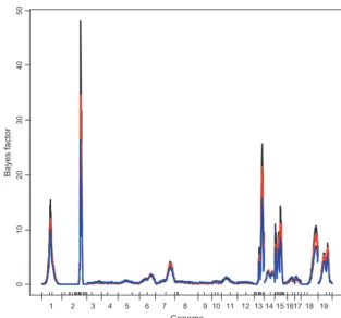
Figure5.—Bayesian epistatic analysis: pro-files of Bayes factor. Black line,l0⫽4; red line, l0⫽6; blue line,l0⫽8. On thex- axis, large tick marks represent chromosomes and small tick marks represent markers.

on chromosomes 2, 13, and 15 overlap those identified tended to provide smaller posteriors, especially for

inquently arising loci. However, the identification of fre-by interval mapping. The graphs of the cumulative

dis-tribution function, displayed in Figure 2, bottom, show quent arising loci remained the same. The profiles of

the Bayes factor are depicted in Figure 5. The three that the posterior inclusion probability of each

chromo-some is close to 1 for chromochromo-somes 2, 13, and 15. The choices oflmprovided similar profiles of the Bayes

fac-tor, especially for infrequently arising loci. results show that, at least in this data set, detection of

large-effect QTL is not sensitive to the choice of lm. As shown in Figures 4 and 5, the epistatic analyses

detected the same regions on chromosomes 2, 13, and

However, larger lm tend to pick up more small-effect

QTL as expected. The profiles of the Bayes factor are 15 as the nonepistatic analyses. In addition to those on

chromosomes 2, 13, and 15, our epistatic analyses found

depicted in Figure 3. For the three choices oflm, the

regions on chromosomes 2, 13, and 15 show strong strong evidence of QTL on chromosomes 1, 18, and

19 with high cumulative probabilities (close to 1) and evidence for being selected, and other regions show a

very low Bayes factor. suggestive evidence of QTL on chromosomes 7 and 14.

In the nonepistatic analyses, these chromosomes were

The epistatic analysis took lm ⫽ 3, the number of

QTL detected in the nonepistatic analyses, as the prior found to have weak main effects and hence were

de-tected in the epistatic model mainly due to epistatic expected number of main-effect QTL . Three values,

l0 ⫽ 4, 6, and 8, were chosen as the prior expected interactions.

The profiles of the location-wise main effects and the number of all QTL under the epistatic model. The

up-per bound of the number of QTL ,L, was thusL⫽10, variances explained by the main effects are depicted in

Figure 6. For the three prior specifications, the posterior 14, and 17, respectively. From Equations 7 and 8, the

prior inclusion probabilities were 0.30, 0.21, and 0.18 inferences were essentially identical. Therefore, we

re-ported only the summary statistics forl0⫽6 (see Tables

for main effects and 0.017, 0.025, and 0.027 for epistatic

effects, for the three values of (l0,L), respectively. The 1 and 2). For the HPD regions on chromosomes 2, 13,

and 15, the posterior inclusion probabilities are close profiles of the posterior inclusion probability for each

locus across the genome and the cumulative posterior to 1, and the corresponding Bayes factors are high. The

estimated main effects were⫺0.856, 0.371, and⫺0.342

probability for each chromosome are depicted in Figure

4, top and bottom, respectively. It can be seen that the and explained 18.4, 3.5, and 3.1% of the phenotypic

variance, respectively. For the HPD regions on

chromo-three different prior specifications of (l0,L) provided

fairly similar profiles of the posteriors, indicating that somes 1, 18, and 19, the posterior inclusion probabilities

were ⵑ82, 88, and 70%, and the corresponding Bayes the posterior inference may be not very sensitive toward

the small or mediate change of l0. As expected, the factors wereⵑ28, 47, and 12, respectively. In these HPD

Figure6.—Bayesian epistatic analysis: profiles of main effect and heritability explained by main effect. Black line,l0⫽ 4; red line, l0 ⫽ 6; blue line, l0 ⫽ 8. On thex- axis, large tick marks represent chromosomes and small tick marks rep-resent markers.

plained low proportions of the phenotypic variance. from relatively short runs. The Bayesian framework

pro-vides a robust inference of genetic architecture that However, our epistatic analyses detected strong epistatic

interactions associated with the HPD regions on chro- incorporates model uncertainty by averaging over all

possible models (Rafteryet al. 1997;Ball2001;

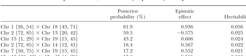
Sil-mosomes 1, 18, and 19. As shown in Table 2, the

strong-est epistasis is the interaction between chromosomes 1 lanpa¨a¨andCorander2002).

and 18. This epistatic effect was estimated to be 0.936 One of the most challenging statistical problems

pre-and explained 5.6% of the phenotypic variance. The pos- sented by QTL mapping is that the number of QTL is

un-terior inclusion probability of this epistasis was 81.9%. known. Most previous Bayesian mapping methods treat

The region of chromosome 19 was found to interact QTL models as models of varying dimension and

em-with chromosomes 15 and 7. The interaction between ploy the reversible jump MCMC algorithm to explore

the regions of chromosomes 19 and 15 was 0.604 and the posterior. Although such a framework is very general

explained 2.5% of the phenotypic variance. The epi- and powerful (Green1995), it is difficult to implement

static analyses also revealed interactions among chromo- efficient search strategies. The key idea of the proposed

somes 2, 13, and 15. For example, the interaction be- Bayesian approach is to turn varying dimensional space

tween the HPD regions on chromosomes 2 and 13 was of multiple-QTL models into fixed dimensional model

included in the model with probability of ⵑ60% and space by using a fixed but large set of known loci,␨,

explainedⵑ2.5% of the phenotypic variance. and putting a constraint on the upper bound of the

number of detectable QTL . In this setting, posterior simulation then can be achieved with a relatively simple

DISCUSSION

Gibbs sampler or M-H algorithm (Godsill 2001; Yi

2004). The algorithm proposed herein is easier to imple-The Bayesian model selection approach provides a

ment than the reversible jump method and it reduces comprehensive solution to mapping multiple epistatic

the computational time of model search, an essential QTL across the entire genome using the posterior

distri-feature for the practical analysis of complex genetic bution as a selection criterion. MCMC algorithms based

architectures. on the composite model space representation mix

rap-A prerequisite of the proposed method is a reasonable idly, thus ensuring that high-probability models are

TABLE 1

Summary statistics for epistatic analysis: high posterior density (HPD) regions of QTL locations, posterior inclusion probabilities of main effects, Bayes factors, estimated main effects,

and heritabilities explained by main effects in the HPD regions

Chromosome

2 13 15 1 18 19 7 14

HPD region (cM) [72, 85] [20, 42] [1, 29] [26, 54] [43, 71] [15, 45] [50, 75] [12, 41]

Posterior probability (%) 98.3 97.2 93.5 81.9 88.4 70.6 36.7 30.1

Bayes factor 821.4 291.3 92.2 28.1 47.3 12.2 4.1 2.7

Main effect ⫺0.856 0.371 ⫺0.342 ⫺0.037 0.103 ⫺0.167 ⫺0.137 ⫺0.147

Heritability 0.184 0.035 0.031 0.002 0.015 0.020 0.019 0.009

QTL . A minimal requirement is that the predetermined to reasonably reduce the model space, such as our

pro-posed composite model space approach, can improve upper bound is greater than the true number of QTL

with high probability. As an extreme case, we could take the performance of the MCMC algorithms and enhance

our ability to detect complex epistatic QTL . We

parti-the total number of loci (H) as the upper bound. Since

the number of detectable QTL is usually much less than tion the entire genome into intervals by a number of

points and restrict putative QTL to these fixed points,

H, such a choice is unlikely to be optimal. The

sugges-tion made here utilizes the expected number of QTL reducing loci to a discrete space. Additional speedup is

achieved by computing the conditional probability of and the prior probability distribution of the number

of QTL to determine the upper bound. The expected the genotypes given the marker data on this fixed (but

dense) grid of possible locations before the MCMC pro-number of QTL could be roughly estimated using

stan-dard genome scans. In practice, one could experiment cedure starts.

Several other strategies of reducing the model space with several values of the expected number of QTL and

investigate their impact on the posterior inference. In could be incorporated into the proposed approach to

improve the procedure. We could adopt a two-stage high-dimensional problems, specifying the prior

distri-butions on both the model space and parameters is search method, first searching for main-effect QTL and

second searching for epistatic effects of these and addi-perhaps the most difficult aspect of Bayesian model

selection. We propose a novel method for elicitation of tional epistatic QTL given the already detected

main-effect QTL . The positions and main main-effects of the QTL prior distribution on the indicator variables. Instead of

directly specifying the prior inclusion probabilitieswm detected in the first stage should be updated in the

second stage since inclusion of epistatic effects may yield

andwe, the expected numbers of main-effect QTL and

all QTL can first be given incorporating previous results more accurate estimation of the positions and the

ef-fects. Alternatively, we could selectively ignore some

ge-and then are used to determine wm and we. Here we

have fixedwmandwebut we could relax this by treating netic effects. Even with a moderate number of

detect-able QTL, the epistatic models must accommodate many

wmandweas unknown model parameters and assigning

priors (Kohnet al.2001). potential genetic effects. In a backcross population, for

example, there are a total ofL(L⫹1)/2 (⫽210, ifL⫽

A major difficulty of genome-wide epistatic analysis

is created by the huge size of the model space. Strategies 20, say) possible effects, but many may be negligible.

TABLE 2

Summary statistics for epistatic analysis: posterior inclusion probabilities of epistatic effects, estimated epistatic effects, and heritability explained by each epistatic effect

Posterior Epistatic

probability (%) effect Heritability

Chr 1 [26, 54]⫻Chr 18 [43, 71] 81.9 0.936 0.056

Chr 2 [72, 85]⫻Chr 13 [20, 42] 59.5 ⫺0.575 0.025

Chr 15 [1, 29]⫻Chr 19 [15, 45] 43.2 0.606 0.024

Chr 2 [72, 85]⫻Chr 14 [12, 41] 18.4 0.567 0.022

Chr 7 [50, 75]⫻Chr 19 [15, 45] 17.2 0.552 0.021

Chr 13 [20, 42]⫻Chr 15 [1, 29] 13.6 ⫺0.501 0.018

M.Wade, B.Brodieand J.Wolf. Oxford University Press, New

To see this, categorize putative QTL into three types:

York.

(1) QTL with main effects (main-effect QTL), (2) QTL _{Chipman, H., E. I. EdwardsandR. E. McCulloch, 2001 The}

practi-cal implementation of Bayesian model selection, pp. 65–116 in

with weak main effects but epistatic effects with other

Model Selection, edited by P. Lahiri. Institute of Mathematical

main-effect QTL , and (3) QTL with weak main effects

Statistics, Beachwood, OH.

but epistatic effects among themselves. Letting the num- _{Fernandez, C., E. LeyandM. F. J. Steel, 2001 Benchmark priors}

for Bayesian model averaging. J. Econom.100:381–427.

bers of these three types of QTL beL1,L2, andL3(L⫽

Gaffney, P. J., 2001 An efficient reversible jump Markov chain

L1 ⫹ L2 ⫹ L3), respectively, and ignoring the main

Monte Carlo approach to detect multiple loci and their effects

effects of (2) and (3) QTL , the number of possible ef- _{in inbred crosses. Ph.D. Dissertation, Department of Statistics,}

University of Wisconsin, Madison, WI.

fects reduces toL1(L1⫹ 1)/2⫹ L1L2⫹L3(L3⫺1)/2

Gelman, A., J. Carlin, H. SternandD. Rubin, 2004 Bayesian Data

(⫽ 115, ifL1⫽ 10, L2 ⫽ 5, andL3 ⫽5). These three

Analysis. Chapman & Hall, London.

types of QTL can be detected either simultaneously or _{George, E. I., 2000 The variable selection problem. J. Am. Stat.}

Assoc.95:1304–1308.

conditionally with a three-stage approach.

George, E. I., andD. P. Foster, 2000 Calibration and empirical

A number of extensions of the basic model are

possi-Bayes variable selection. Biometrika87:731–747.

ble within this framework. The simplicity of the MCMC _{George, E. I., andR. E. McCulloch, 1997 Approaches for Bayesian}

variable selection. Stat. Sin.7:339–373.

search enhances the overall flexibility of this approach

Godsill, S. J., 2001 On the relationship between MCMC model

and enables one to consider analysis in more complex _{uncertainty methods. J. Comput. Graph. Stat.10:230–248.}

settings. Extensions to binary or ordinal traits, inclusion Green, P. J., 1995 Reversible jump Markov chain Monte Carlo

com-putation and Bayesian model determination. Biometrika 82:

of fixed- or random-effect covariates, and

gene-by-envi-711–732.

ronment interactions are feasible. In principle, the com- _{Heath, S. C., 1997 Markov chain Monte Carlo segregation and}

posite space method can be directly applied to identify linkage analysis for oligogenic models. Am. J. Hum. Genet.61:

748–760.

higher-order interactions. However, the dramatic

in-Hoeschele, I., 2001 Mapping quantitative trait loci in outbred

pedi-crease in the size of model space is likely to limit the _{grees, pp. 599–644 inHandbook of Statistical Genetics, edited by}

performance of the MCMC algorithm. We regard the D. J.Balding, M.Bishopand C.Cannings. Wiley, New York.

Jansen, R. C., 2003 Studying complex biological systems using

multi-methods proposed here as a step toward achieving more

factorial perturbation. Nat. Rev. Genet.4:145–151.

efficient and comprehensive analysis of complex genetic _{Jansen, R. C., andP. Stam, 1994 High resolution of quantitative traits}

architectures. There are many opportunities to extend into multiple loci via interval mapping. Genetics136:1447–1455.

Jiang, C., andZ-B. Zeng, 1997 Mapping quantitative trait loci with

and improve upon this general approach.

dominant and missing markers in various crosses from two inbred N.Y. and D.B.A. were supported by National Institutes of Health (NIH) lines. Genetica101:47–58.

Kadane, J. B., andN. A. Lazar, 2004 Methods and criteria for model grants NIH RO1GM069430, NIH RO1ES09912, NIH RO1 DK056366,

selection. J. Am. Stat. Assoc.99:279–290. NIH P30DK056336, and an obesity-related pilot/feasibility studies

Kao, C. H., andZ-B. Zeng, 2002 Modeling epistasis of quantitative grant at the University of Alabama (Birmingham) (528176). G.A.C.

trait loci using Cockerham’s model. Genetics160:1243–1261. was supported by NIH GM070683. B.S.Y. was supported by NIH/

Kao, C. H., Z-B. ZengandR. D. Teasdale, 1999 Multiple interval National Institute of Diabetes and Digestive and Kidney Diseases _{mapping for quantitative trait loci. Genetics152:1203–1216.} (NIDDK) 5803701, NIH/NIDDK 66369-01, American Diabetes Associ- _{Kass, R. E., andA. E. Raftery, 1995 Bayes factors. J. Am. Stat. Assoc.} ation 7-03-IG-01, and U.S. Department of Agriculture Cooperative _{90:773–795.}

State Research, Education and Extension Service grants to the Univer- Kohn, R., M. SmithandD. Chen, 2001 Nonparametric regression using linear combinations of basis functions. Stat. Comput.11:

sity of Wisconsin (Madison) (C.J. and B.S.Y.). This research is a

con-313–322. tribution of the University of Nebraska Agricultural Research Division

Kuo, L., andB. Mallick, 1998 Variable selection for regression (Lincoln, NE; journal series no. 14858) and the North Carolina

Ag-models. Sankhya Ser. B60:65–81. ricultural Research Service and was supported in part by funds

pro-Lander, E. S., andD. Botstein, 1989 Mapping Mendelian factors vided through the Hatch Act.

underlying quantitative traits using RFLP linkage maps. Genetics

121:185–199.

Leamy, L. J., D. Pomp, E. J. EisenandJ. M. Cheverud, 2002 Pleiot-ropy of quantitative trait loci for organ weights and limb bone lengths in mice. Physiol. Genomics10:21–29.

LITERATURE CITED

Lynch, M., andB. Walsh, 1998 Genetics and Analysis of Quantitative

Ball, R. D., 2001 Bayesian methods for quantitative trait loci map- _{Traits. Sinauer Associates, Sunderland, MA.}

ping based on model selection: approximate analysis using the _{Narita, A}., andY. Sasaki, 2004 Detection of multiple QTL with Bayesian information criterion. Genetics159:1351–1364. epistatic effects under a mixed inheritance model in an outbred

Bogdan, M., J. K. GhoshandR. W. Doerge, 2004 Modifying the population. Genet. Sel. Evol.36:415–433.

Schwarz Bayesian information criterion to locate multiple inter- Raftery, A. E., D. Madiganand J. A. Hoeting, 1997 Bayesian acting quantitative trait loci. Genetics167:989–999. model averaging for linear regression models. J. Am. Stat. Assoc.

Broman, K. W., andT. P. Speed, 2002 A model selection approach 92:179–191.

for identification of quantitative trait loci in experimental crosses. Reifsnyder, P. R., G. ChurchillandE. H. Leiter, 2000 Maternal J. R. Stat. Soc. B64:641–656. environment and genotype interact to establish diabesity in mice.

Carlborg, O., andC. Haley, 2004 Epistasis: Too often neglected Genome Res.10:1568–1578.

in complex trait studies? Nat. Rev. Genet.5:618–625. Satagopan, J. M., andB. S. Yandell, 1996 Estimating the number of

Carlborg, O., L. AnderssonandB. Kinghorn, 2000 The use of quantitative trait loci via Bayesian model determination. Special a genetic algorithm for simultaneous mapping of multiple inter- Contributed Paper Session on Genetic Analysis of Quantitative acting quantitative trait loci. Genetics155:2003–2010. Traits and Complex Disease. Biometric Section, Joint Statistical

Carlin, B. P., andS. Chib, 1995 Bayesian model choice via Markov Meeting, Chicago.

chain Monte Carlo. J. Am. Stat. Assoc.88:881–889. Satagopan, J. M., B. S. Yandell, M. A. NewtonandT. C. Osborn,

Cheverud, J. M., 2000 Detecting epistasis among quantitative trait 1996 A Bayesian approach to detect quantitative trait loci using Markov chain Monte Carlo. Genetics144:805–816.

Sen, S., andG. Churchill, 2001 A statistical framework for quantita- _x

iq1⫽ziq⫺ 1, tive trait mapping. Genetics159:371–387.

Sillanpa¨a¨, M. J., andE. Arjas, 1998 Bayesian mapping of multiple _x

iq2⫽(1⫹ xiq1)(1⫺xiq1)⫺0.5, quantitative trait loci from incomplete inbred line cross data.

Genetics148:1373–1388.

Sillanpa¨a¨, M. J., andJ. Corander, 2002 Model choice in gene mapping: what and why. Trends Genet.18:301–307.

xiqq⬘k⫽

⎧ ⎪ ⎨ ⎪ ⎩

xiq1xiq⬘1, k⫽ 1

xiq1xiq⬘2, k⫽ 2

xiq2xiq⬘1, k⫽ 3

xiq2xiq⬘2, k⫽ 4 .

Stephens, D. A., andR. D. Fisch, 1998 Bayesian analysis of quantita-tive trait locus data using reversible jump Markov chain Monte Carlo. Biometrics54:1334–1347.

Thomas, D. C., S. Richardson, J. GaudermanandJ. Pitkaniemi,

1997 A Bayesian approach to multipoint mapping in nuclear _{For the Cockerham model,} ␤_q1and ␤_{q2 correspond to} families. Genet. Epidemiol.14:903–908.

additive and dominance effects of QTLq, respectively;

Uimari, P., andI. Hoeschele, 1997 Mapping linked quantitative

and␤qq⬘1,␤qq⬘2,␤qq⬘3, and␤qq⬘4are the epistatic effects be-trait loci using Bayesian method analysis and Markov chain Monte

Carlo algorithms. Genetics146:735–743. _{tween lociqandq}⬘_{, called by-additive,}

additive-Yi, N., 2004 A unified Markov chain Monte Carlo framework for

by-dominance, by-additive, and

dominance-mapping multiple quantitative trait loci. Genetics167:967–975.

by-dominance effects, respectively. The Cockerham model

Yi, N., andS. Xu, 2000 Bayesian mapping of quantitative trait loci

for complex binary traits. Genetics155:1391–1403. _{keeps the same interpretation of main effects with or}

Yi, N., andS. Xu, 2002 Mapping quantitative trait loci with epistatic

without epistatic effects. However, main effects should

effects. Genet. Res.79:185–198.

always be interpreted with caution in the presence of

Yi, N., D. B. AllisonandS. Xu, 2003 Bayesian model choice and

search strategies for mapping multiple epistatic quantitative trait _{epistatic interactions.} loci. Genetics165:867–883.

Yi, N., A. Diament, S. Chiu, J. FislerandC. Warden, 2004a Charact-erization of epistasis influencing complex spontaneous obesity

in the BSB model. Genetics167:399–409. _{APPENDIX B: THE PRIOR EXPECTED NUMBER OF}

Yi, N., A. Diament, S. Chiu, J. FislerandC. Warden, 2004b Epistatic _{QTL INCLUDED IN THE MODEL} interaction between chromosomes 7 and 3 influences hepatic

lipase activity in BSB mice. J. Lipid Res.45:2063–2070. _{We define␰}

qas the binary variable to indicate

inclu-Zeng, Z-B., 1994 Precision mapping of quantitative trait loci.

Genet-sion (␰q⫽1) or exclusion (␰q⫽0) of QTLq. QTLqis

ics136:1457–1468.

included into the model when and only when at least

Zeng, Z-B., C. KaoandC. J. Basten, 2000 Estimating the genetic

architecture of quantitative traits. Genet. Res.74:279–289. _{one of the genetic effects associated with QTL qis}

in-cluded. Therefore, we have

Communicating editor: J. B.Walsh

␰q⫽1⫺

兿

K

k⫽1

(1 ⫺ ␥qk)

兿

K2

k⫽1

冤

兿

L

q⬘⬎q

(1⫺ ␥qq⬘k)

兿

L

q⬘⬍q

(1 ⫺ ␥q⬘qk)

冥

,

APPENDIX A: THE MODIFIED COCKERHAM EPISTATIC MODEL FOR BACKCROSS AND

whereKis the number of possible main effects for each

INTERCROSS POPULATIONS

locus,K2_{is the number of possible epistatic effects for}

For a mapping population withK⫹1 genotypes per

any two loci, and␥qkand␥qq⬘kare the indicators of main

locus, there are Kmarginal effect degrees of freedom

and epistatic effects, respectively. The actual number of

(d.f.) for each locus and K2 _{interaction-effect d.f. for}

QTL then equals 兺L

q⫽1␰q. The prior expected number

any two loci. The design matrixXfor model (1) hasKL

of all QTL is the expectation of the actual number of

main-effect coefficients,xiqk, andK2L(L⫺1)/2 epistatic

QTL and thus can be derived as

effect coefficients,xiqq⬘k, obtained from the genotypes at

the corresponding loci by using a particular epistatic _l

0⫽

兺

L

q⫽1

pr(␰q⫽1) model. The main and epistatic effects are denoted by

␤qkand␤qq⬘k, respectively.

⫽L⫺

兺

L

q⫽1

冦

兿

K k⫽1

pr(␥qk⫽0)

兿

K2

k⫽1

冤

兿

L

q⬘⬎q

pr(␥qq⬘k⫽0)

兿

L

q⬘⬍q

pr(␥q⬘qk⫽0)

冥冧

For a backcross population, there are two segregating

genotypes denoted bybqbq,Bqbqat locusq. For the

com-⫽L[1⫺(1⫺wm)K(1⫺we)K

2_(L⫺1)

] .

monly used Cockerham epistatic model (KaoandZeng

2002), the coefficients are defined as _{If we consider only main effects, then QTLqis included}

into the model when at least one of the main effects of

xiq1⫽ziq⫺ 0.5 and xiqq⬘1⫽xiq1xiq⬘1,

QTLqis included. The binary indicator variable of QTL

where ziq denotes the number of allelesBq. For an

in-qthen becomes␰q⫽ 1⫺ ⌸

K

k⫽1(1⫺ ␥qk). Therefore, the

tercross derived from two inbred lines, there are three

prior expected number of main-effect QTL is

segregating genotypes denoted bybqbq,Bqbq, andBqBqat

locus q. For the commonly used Cockerham epistatic _l

m⫽L⫺

兺

L

q⫽1

冤

兿

K k⫽1

pr(␥qk⫽0)

冥

⫽L[1⫺(1 ⫺w_m)K].