Impact of Nonrandom Mating on Genetic Variance and Gene Flow in Populations With Mass Selection



Impact of Nonrandom Mating on Genetic Variance and Gene Flow in

Populations With Mass Selection

Leopoldo Sa´nchez

1

_{and John A. Woolliams}

Roslin Institute (Edinburgh), Roslin, Midlothian EH25 9PS, United Kingdom Manuscript received March 19, 2002

Accepted for publication September 19, 2003

ABSTRACT

The mechanisms by which nonrandom mating affects selected populations are not completely under-stood and remain a subject of scientific debate in the development of tractable predictors of population characteristics. The main objective of this study was to provide a predictive model for the genetic variance and covariance among mates for traits subjected to directional selection in populations with nonrandom mating based on the pedigree. Stochastic simulations were used to check the validity of this model. Our predictions indicate that the positive covariance among mates that is expected to result with preferential mating of relatives can be severely overpredicted from neutral expectations. The covariance expected from neutral theory is offset by an opposing covariance between the genetic mean of an individual’s family and the Mendelian sampling term of its mate. This mechanism was able to predict the reduction in covariance among mates that we observed in the simulated populations and, in consequence, the equilib-rium genetic variance and expected long-term genetic contributions. Additionally, this study provided confirmatory evidence on the postulated relationships of long-term genetic contributions with both the rate of genetic gain and the rate of inbreeding (⌬F) with nonrandom mating. The coefficient of variation of the expected gene flow among individuals and⌬Fwas sensitive to nonrandom mating when heritability was low, but less so as heritability increased, and the theory developed in the study was sufficient to explain this phenomenon.

R

ECENT advances in quantitative genetic theory female, has been less well studied in this context. Al-though utilizing a mating design to minimize⌬F does have allowed breeding schemes to consider the

not always lead to substantial deviations from HW pro-management of genetic variation objectively,

simultane-portions (Sonesson and Meuwissen 2000), much of ously with the maximization of genetic gain. Such

ad-the ad-theory on genetic variation and ad-the impact of non-vances are highly relevant to breeding practice, not only

random mating has been built up around the concept for commercial schemes but also for those schemes that

of departures from HW equilibrium (e.g., Caballero

are orientated toward the conservation of genetic

re-andHill1992;SantiagoandCaballero1995;Wang

sources. These advances include the development of

1996) and the concepts of the avoidance of, or prefer-tractable, deterministic predictors of rates of inbreeding

ence for, mating relatives. (⌬F), gene flow, and genetic gain (⌬G) for complex

The interpretation of the work on nonrandom mat-selected populations (Woolliamset al. 1999;

Woolli-ing, both its application and its impact, remains a subject

ams and Bijma 2000), and operational tools for

day-of scientific debate. For example, in conservation, ac-to-day selection decisions (Wray andGoddard 1994;

cepted practice uses minimum coancestry to minimize

Meuwissen1997;Grundyet al. 1998).

⌬F (Caballeroet al. 1996;Frankhamet al.2002), yet However, the theory underpinning these tools has

recent theoretical developments using genetic contribu-been developed primarily for random mating of the

tions show that the lowest⌬Fwith hierarchical matings selected males and females and for a neutral locus where

is achievable when relatives are preferentially mated the genotypic frequencies in the offspring display no

(Sa´nchezet al. 2003). In selected populations, there is departure from Hardy-Weinberg (HW) proportions,

clear evidence that mating designs are beneficial, al-other than that arising from the partitioning of the gene

though not all these designs define matings through pool induced by two sexes (Robertson1965). However,

pedigree, e.g., factorial mating (Woolliams 1989). the role of nonrandom mating, where some specific

Several articles indicate that attention to the pedigree design is placed upon which male is mated to which

relationships within a mating design can be advanta-geous over random-mating schemes (e.g.,Santiagoand

Caballero1995;Caballeroet al. 1996;Sa´nchezet al.

1_{Corresponding author: INRA-Orle´ans, Unite´ d’Ame´lioration,}

Ge´n-1999). However, the benefits of these methods have not

e´tique et Physiologie des Arbres Forestiers, Ave. de la Pomme de Pin,

always been quantified in predictable terms for their

Ardon, B.P. 20619-45166 Olivet Cedex, France.

E-mail: [email protected] joint impact upon genetic gain and rates of inbreeding.

viduals), it measures the actual loss of heterozygosity due to Moreover, other studies on mating designs (Toroand

the nonrandomness of the mating of the parents with nonzero Pe´rez-Enciso1990;Klieveet al. 1994;Ferna´ndezand

contributions in the offspring generation (often denoted as Toro1999) do not separate out the impact of specifying _␣

I). Thus the former (␣O) is a potential correlation of uniting the matings from the impact of controlling only the _{gametes from selected parents, whereas the latter (␣I) is a} realized correlation and will be affected by the finite random overall contribution of each selected individual

assum-sampling of gametes to form the offspring generation and ing random mating.

by any artificial and/or natural selection of offspring before SantiagoandCaballero(1995) were successful in

reaching the breeding population.

producing predictions of the effective population size _{Under the assumption of completely neutral genes␣} Owould [Ne, defined as (2⌬F)⫺1] in nonrandom mating popula- tend to be equal to␣I. For neutral genes, when nonrandom

mating results from a mix of full-sib mating and random mat-tions undergoing mass selection, using an approach

ing,␣I(i.e.,␣I⬇␣O⫽ ␣) can be related to the proportion of based upon the variance of allele frequencies. These

full-sib mating (denoted hereafterφ) by␣ ⫽φ/(4⫺3φ) (Ghai authors considered nonrandom mating in the form of

1969). departures from HW equilibrium achieved through par- _{To obtain␣}

Oin a breeding population, let␪ijbe the

coances-tial full-sib mating. However, Woolliams and Bijma try (kinship) coefficient (LynchandWalsh1998) of sireiand damj, then followingWright’s (1969) equation 1⫺ ␣O(i,j)⫽ (2000) showed that, for random mating, an approach

(1⫺ ␪ij)/(1⫺ ␪), where␪ ⫽FSTis the average of all the entries to predictingNeusing long-term genetic contributions

in the matrix of coancestries among the parents (i.e.,i,j, and was capable of extension to more complex selection

contemporaries), including self-coancestries and the recipro-schemes. To achieve such an extension with nonrandom _{cals (Cockerham1967). Thus␣}

O(i,j)is defined for any pair of mating requires an understanding of the expected gene _{parents in relation to the complete set of selected parents.} The term ␣O is the average ␣O(i,j) of the selected matings, flows of individuals based upon the inheritance of

selec-irrespective of the fitness of the offspring,i.e., as if all matings tive advantages, which in turn presupposes an

understand-contribute an equal and large number of offspring to the next ing of the behavior of the genetic variation. There appears

generation.

to be little published information on these topics. _{To obtain a summary value of␣}

Ifor a pedigreed population Therefore, the main objective of this study is to ad- _{undergoing selection, we follow the same reasoning as above.} Note that␪ ⫽FSTrepresents the average inbreeding coeffi-vance the theoretical framework for predicting the

im-cient if the offspring generation had been obtained by com-pact of nonrandom mating for populations undergoing

plete aggregation of the parental gene pool and sampling at directional selection, providing a predictive model for

random with replacement. Then for any individual offspring the genetic variance and covariance among mates. The _{from that set of parents ␣}

I(k) ⬇ FIS and can be defined as nonrandom mating is defined solely in terms of depar- 1⫺ ␣I(k)⫽(1⫺F(k))/(1⫺ ␪), whereF(k) is the coefficient

of inbreeding of individualk, and is equal to␪sire(k),dam(k). For tures from HW proportions for neutral alleles, without

the infinitesimal model, the Mendelian sampling deviation reference to phenotypes. The impact is measured in

for an offspringkhas a variance equal to terms of genetic parameters, such as genetic variance,

expected gene flow, and⌬F, assuming the infinitesimal 1 2␴

2 A,0

冢

1⫺1

2F(sire(k))⫺ 1

2F(dam(k))

冣

⫽ 1 2␴

2 A,0

冤

1

2(1⫺F(sire(k)))⫹ 1

2(1⫺F(dam(k)))

冥

model and mass selection. In the course of this article,

the opportunity to validate the developments ofWool- ⫽1

2␴

2

A,0(1⫺ ␪)

冢

1⫺1

2␣I(sire(k))⫺ 1

2␣I(dam(k))

冣

, (1)

liams and Bijma (2000) for nonrandom mating is

where␴2

A,0is the initial variance of the breeding values. In the taken. The accuracies of the predictions of⌬Fand⌬G

remainder of this study, the term (1⫺ ␪) in Equation 1 is and the validity of the framework are established with

omitted for derivations and predictions, analogously to

Wool-the help of stochastic simulations. _{liamset al. (1999) andWoolliamsandBijma(2000). This}

omission allows the genetic variance to reach an equilibrium. Further details are given in the last section ofmaterials and methods.

MATERIALS AND METHODS

The terms␣I(k)are used to define two related, but distinct,

Nonrandom mating and neutral theory: The correlation _{summary ␣I: (i) ␣Ic ⫽ 兺kck␣I(k), where ck was the observed} between uniting gametes due to the nonrandom mating of contribution ofkto the selected offspring in the next genera-parents is an additional factor affecting heterozygosity over tion, and (ii)␣Ir⫽兺krk␣I(k), whererkwas the long-term genetic and above initial gene frequencies and their accumulated contribution (described in the following sections) ofk. If we drift. Using the classical F-statistics of Wright (1969), the assume now that directional selection has taken place among expected fractional decrease in the heterozygosity for a given families, then the direct equivalence between␣Oand␣I

(irre-population (FIT) can be related to two further statistics using spective of whether Ic or Ir) no longer holds for selective

the relationship (1⫺FIT)⫽(1⫺FIS)(1⫺FST), whereFSTis genes or neutral genes since selection success will depend on

the fractional loss of heterozygosity due to the finiteness of the␣Iof the parents (Caballeroet al. 1996).

the population census, andFISis the loss of heterozygosity due Dynamics of genetic (co)variance for a selected trait under

to the nonrandom mating of parents. TheFIScan be seen as nonrandom mating:In this section, a model is developed to

a correlation of gene effects between homologous alleles in show that the impact of nonrandom mating on covariances pairs of mating parents,i.e., the correlation between alleles between mates for selected traits and neutral traits may be within infinitely many conceptual offspring derived from each qualitatively different and to describe the circumstances under of the pairs of mating parents (often denoted␣Oand hereafter which this can occur. In particular, it demonstrates that

indi-selected parents but also between a parent and its mate, from Equation 3 is that the covariance between mates for the selected trait may be dramatically reduced below what is thereby reducing genetic variance more than would be

pre-dicted by previously existing selection theory. expected whenbafbecomes more strongly negative, when (i) selection intensity is large, since␬ →1, and when (ii)h2

0is

Consider a population with equal numbers of dams and

sires,i.e., a mating ratio of 1, mated in pairs to produce a large, since ␴2

M/␴2P is large. The term (1⫹baf)2is relatively insensitive to␣for mass selection, but is sensitive toh2

0. For

deviation from HW equilibrium equal to␣Oon the basis of

pedigree information alone. For the trait under selection, assume ␬ ⫽0.64,␣ ⫽0.06, (1⫹baf)2takes values of 0.87, 0.73, 0.57, 0.38, and 0.18 forh2

0⫽0.2, 0.4, 0.6, 0.8, and 0.99, respectively

a heritability ofh2

0when in HW equilibrium in an unselected

base generation, with a phenotypic variance␴2

P,0⫽1. It is as- (from Equation 3 and genetic variances obtained from

simu-lated populations); for␣ ⫽ 0.24, the values are 0.90, 0.77, sumed that the inheritance of the trait under selection can

be described by an infinitesimal model and, for simplicity in 0.62, 0.42, and 0.18. Since ␴2_*

M ⫽ ␴2M(1⫺ ␬␴2M/␴2P),␴A2*⫽ ␴2F*⫹2 cov(fi,ai)*⫹ the derivation of this model, that the nonrandom mating is

achieved by managingφ, the proportion of full-sib matings. ␴2_*

M ⫽ ␴2A(1⫺ ␬h2), and for their offspringAoff⫽1⁄2(Ai⫹Aj)⫹

aoff:

Note that this mating scheme does not produce half-sibs. From Ghai(1969), the neutral expectations are␣I⫽ ␣O⫽ ␣, and

␴2

A⫽1⁄2(␴2A*⫹φ(1⫹baf)2␴2F*)⫹ ␴2M. (5)

φ⫽4␣/(1⫹3␣) for large populations.

LetPidenote the phenotype of an individualifor the se- _{This will move to equilibrium over generations so that the} lected trait andBibe the breeding value for a neutral trait, _{effect of selection is counterbalanced by the addition of}␴2

M

then the covariance between breeding values of mates is given _{(analogously toBulmer1980, p. 155).}

byCaballero and Hill (1992) as cov(Bsire, Bdam)⫽ 2␣O␴2B, _{Consequently, for the selected trait, the total observed}

addi-where␴2

Bis the variance of the breeding values in the unse- _{tive variance may decline even as}␣

Oincreases (demonstrated

lected and randomly mated base population. Now consider _{in theresults), although ␣}

Ois superficially increasing one Ai, the breeding value for the selected trait. ThenAi⫽1⁄2(Asire⫹ _{component of the variation. This is a phenomenon associated} Adam)⫹ai⫽fi⫹ai, wherefiis the true family mean, andai _{with linkage disequilibrium and arises from (i) a lower} Mende-is the Mendelian sampling term. Define␴2

A,tas the variance _{lian sampling variance replenishing the genetic variation lost} of the breeding values at timetwith␴2

A,t⫽ ␴2F,t⫹ ␴2M, where _{due to selection in each generation and (ii) the induction of}

␴2

F,t is the variance of the true family means at timet, and _{negative covariance between the Mendelian sampling term of} ␴2

M⫽1⁄2(1⫺ ␣I)h20is the variance of the Mendelian sampling _{a parent and the true family mean of its mate.}

terms [note that the term (1⫺ ␪) in Equation 1 is omitted _{Predictions of rate of inbreeding and genetic gain through} here, and since␴2

P,0⫽1,h20⫽ ␴2A,0]. For simplicity, the explicit _{the concept of long-term genetic contributions:The genetic}

dependence ontin the notation is neglected. For selection _{contribution of an ancestork(denotedr}

k) to a descendantj on phenotypePi, _{is the proportion of genes carried byj that are expected to} derive by descent from the ancestork. A descendant’s breeding fi⫽ ␴

2 F

␴2 P

Pi⫹εi,1 _{value can be decomposed into a sum of Mendelian sampling}

deviations from all ancestors, with the weighting for ancestor k’s Mendelian deviation being rk. For a mixing population,

ai⫽ ␴

2 M

␴2 P

Pi⫹εi,2, (2) _{after a sufficiently large number of generations,k’s genetic}

contribution to all individuals within the population ap-wherefiandaiare both partitioned into an expectation condi- proaches the same stable and constant value across genera-tional onPiand a residual (ε). Since cov(fi,ai)⫽0, cov(ε1,ε2)⫽ tions. In the remainder of the text, the stable genetic

contribu-⫺␴2

F␴2M/␴2P. Following the methods ofBulmer(1980) for selec- tions from distant ancestors are referred to as “long-term

tion with the infinitesimal model, let superscript * denote a genetic contributions.” The long-term genetic contributions parameter postselection onPi, then cov(fi,ai)*⫽ ⫺␬␴2F␴2M/␴2P will reflect differences among individual ancestors arising

since␴2*

P ⫽(1⫺ ␬)␴2P, where␬is the variance reduction coef- from their respective selective advantages together with

cumu-ficient. This has a direct analogy to linkage disequilibrium, lative chance factors across generations. Therefore, long-term where selection onPiinduces negative covariance between genetic contributions model the gene flow of individual ances-the effects of different loci, and where ances-the induction of this tors through the population.

covariance is not dependent on mating procedures. The re- The asymptotic⌬Ffor nonrandom mating can be derived gression ofaionfiafter selectionis through its theoretical relationship with the sum of squared

long-term genetic contributions, baf⬇⫺␬␴2F␴2M/(␴2P␴2F*) , (3)

⌬F⫽1_⁄

4(1⫺ ␣I)

兺

k

r2

k (6)

where␴2_*

F ⫽ ␴2F(1⫺ ␬␴2F/␴2P) is the variance of true full-sib family

means after selection. Notebaf⬍0, andbaf⬆0 after selection.

(WoolliamsandBijma2000). The rate of genetic gain (⌬G) When allocating mates (i, j) using the pedigree alone,

per generation is also related to long-term genetic

contribu-cov(Ai,Aj)⫽cov(fi⫹ai,fj⫹aj) tions since sustained genetic gain arises through the

genera-tion of covariance between long-term genetic contribugenera-tions ⫽cov(fi,fj)⫹cov(fi,aj)⫹cov(fj,ai)⫹cov(ai,aj). _{and Mendelian sampling deviations,}

Substitutingaj⫽baffj⫹εjand analogously forai, and usingφ _⌬

G⫽

兺

k

rkak (7)

to estimate the covariance between mates,

cov(Ai,Aj)⫽φ␴2F*⫹2bafφ␴2F*⫹b2afφ␴2F* _{(Woolliamset al. 1999), where the sum is taken over a}

genera-tion of ancestors. Therefore, the concept of long-term genetic ⫽φ␴2_*

F (1⫹baf)2. (4)

contribution bridges the loss of heterozygosity and the genera-tion of genetic gain for any deviagenera-tion from random mating In the absence of selection, this is simplyφ␴2

F. Therefore, with

selection, since (i)␴2_*

F ⬍ ␴2Fand (ii)baf⬍0, the covariance given by␣I.

For mass selection, the selective advantages for an ancestor achieved between the breeding values of mates for the trait

selective advantages influences not only the breeding success leading to sublining. For the benefit of a more general scheme, the upper limit of ␣Ofix was ⬍1 in this study. On the other

of the resulting offspring from that given ancestor, but also

that of subsequent descendants. This dependence of the gene extreme, the lowest possible value of␣Oin finite populations

lies much closer to what is expected for random-mating popu-flow on the selective advantage can be expressed as a

condi-tional expectation (␮k),i.e., as a function of the selective advan- lations, due to the fact that the avoidance of inbreeding is constrained in the long term by the genetic depletion caused tages. For truncation selection based upon phenotype,␮kcan

be satisfactorily modeled as a linear relationship between the by drift, as pointed out byCaballeroandHill(1992). The values of␣Ofixused in the simulation were⫺0.03, 0, 0.03, 0.06,

genetic contribution and the breeding values,

0.12, 0.18, and 0.24. ␮k⫽ ␥ ⫹ ␤(r,A)(Ak⫺A)⫹ ␤⬘(r,A)

兺

mates(Amate(k)⫺A

⬘) (8) _{Long-term genetic contributions were calculated for an}

an-cestral generation born after 20 generations of selection from (Woolliamset al. 1999), where the termsAand A⬘ are the _{the unselected base and upon the cohort of descendants born} mean breeding values of the selected individuals for the sex _{20 generations after that ancestral generation. This} guaran-ofkand its mates’ sex, respectively. For discrete generations, _{teed attainment of equilibrium of genetic variances in all the} ␥ ⫽(2NS)⫺1and (2ND)⫺1forNSsires andNDdams, respectively, _{cases with}␣_Ofix ⱕ_{0.12. With more extreme}␣_{Ofix, however, a}

and is independent ofh2

0and␣I. WhenNS⫽ND⫽Nwith no _{longer period of time was needed before such equilibrium is}

mating hierarchy, ␤(r,A)⫽ ␤⬘(r,A), and from here onward, we _{reached (Santiago and Caballero1995). For these cases,}

denote this as␤. Therefore under these two conditions, dis- _{20 further generations were bred before establishing the} an-crete generations and N mating pairs, the only parameters _{cestral generation, although it was found unnecessary to} ex-varying with the breeding scheme are the slope of the relation- _{tend the period of time for obtaining summary statistics for the} ship ␤and the genetic variance among selected individuals _{converged contributions (i.e., 20 generations from ancestors to} derived from␴2

A(Woolliamset al. 1999). Equation 8 becomes _{descendants). Observed long-term genetic contributions were}

used to calculate the predictions of⌬Fand⌬Gfrom Equations ␮k⫽ ␥ ⫹ ␤[(Ak⫺A)⫹(Amate(k)⫺A⬘)]. (9)

6 and 7.

The values of achieved␣O,␣Ic,␣Ir, and␴2Aand the genetic

Thus␤is the regression coefficient of the long-term

contribu-covariance among mates were recorded for each generation tion of an individual on the sum of its breeding value and that

of the simulated populations, together with the observed⌬F, of its mate. The impact of the selective advantage on the gene

⌬G, 兺r2

k, and 兺rkak (Equation 7). The observed⌬F and ⌬G flow (and, ultimately, on ⌬F) can then be measured by the

were obtained as the average rate of the last 20 generations coefficient of variation (CV) of the conditional expectation:

of the simulated populations.␤was obtained by multiple re-CV(␮k)⫽2N␤√2(␴2A*⫹φ(1⫹baf)2␴2F*) . (10) _{gression of the long-term contribution of ancestors on their}

own breeding value and that of their mates; as no significant Population model and procedures for stochastic simulation:

difference in the regression coefficients was found, as pre-This section describes the general population model and

selec-dicted, the value used in the text is the average of the two tion procedures for which predictions and simulations will

values. The proportion of full-sib matings (φ) was also re-be compared. The population was reproduced in discrete

corded in each simulated population. Results were averaged generations with a constant breeding size ofNSsires andND

over 1000 replicates and standard errors derived from the dams and a mating ratio of dams to sires of 1 in all generations

variance between replicates. The values of basic parameters (NS⫽ND⫽N). Each dam motherednOoffspring, all full-sibs,

used in the simulations wereh2

0⫽{0.01, 0.05, 0.1, 0.2, 0.4, 0.6,

and comprising equal numbers of male and female candidates.

0.8, and 0.99},N⫽{32, 64, and 128}, andnO⫽{4, 8, and 16}.

Selection was upon phenotypeP, which was the sum of breed-ing valueAand an environmental deviation.

For simulation, a noninbred and unrelated base population was generated with␴2

P,0⫽1. Each founder’sAwas taken from RESULTS N(0,␴2

A,0), where ␴2A,0 is the initial genetic variance (since

␴2

P,0⫽1, initial heritabilityh20⫽ ␴2A,0). In subsequent generations, Expectedvs. observed degree of nonrandom mating:

each new breeding value was the sum of1_⁄

2(Asire⫹Adam) and a The degree of nonrandom mating is described in this

Mendelian sampling deviation. The latter term was drawn from _{section, in terms of (i) the two distinct summary␣}

I’s (i.e., N(0,1_⁄

2␴2A,0(1⫺1⁄2␣I(sire)⫺1⁄2␣I(dam))), where␣I(sire)and␣I(dam)are _␣

Icand␣Ir)vs.␣Ofixand (ii) the expected and observed

due to the nonrandom mating between grandparents. An

envi-proportion of full-sib matings (φexpandφobs, respectively).

ronmental deviation sampled fromN(0, 1⫺ ␴2

A,0) was added to

each individual’s breeding value to obtainP. The simulations For item i, Table 1 shows that substantial deviations omitted the term (1⫺ ␪) in Equation 1, as previously indicated _{between ␣Ir and ␣Ic occurred, with ␣Ir ⬍ ␣Ic as h}2

0

in-in the first section. Consequently, the genetic variance, and

creased and ␣Ofixincreased. Statistically significant but

hence the variance in the selective advantages, in the simulated

slight differences with ␣Ir ⬎ ␣Ic also occurred with h20 ⫽

populations reached an equilibrium upon which to base stable

0.01. Where␣Ir⬍ ␣Ic, the substantial difference indicates predictions.

Selected individuals were mated following a mating design a negative covariance between the individual’s long-with nonrandom mating based upon␣O(as defined earlier), _{term genetic contribution and}␣_{I. Thus, those}

individu-which was carried out systematically in all generations except

als with low values of␣I, consequently with a relatively

in the base population, where founders were randomly

allo-greater Mendelian sampling variance in their offspring, cated in pairs. The allocation of mates was decided in such a

had a selective advantage over their contemporaries way that ␣O was as close as possible to a target value ␣Ofix.

This process involved a search throughout the feasible set of and, therefore, a greater long-term genetic contribu-matings, carried out by the simulated annealing technique _{tion. This association between long-term genetic} contri-(Presset al. 1992), to minimize the objective function given

butions and the variation in␣Iwithin a scheme became

by (␣O⫺ ␣Ofix)2. A random sample of matings was used as a

more evident as selection became more intense, through starting point. The maximum feasible value for␣Ois 1, which

TABLE 1

Target departures from HW proportions (␣Ofix)vs.observed departures measured as the asymptotic average

of␣Iweighted by the observed contribution as parent to the selected offspring in the next generation (␣Ic)

and the asymptotic average of␣Iweighted by the long-term genetic contribution (␣Ir), with phenotypic

selection andN⫽32, for different␣Ofix, family size (nO), and initial heritabilities (h20)

h2

0⫽0.01 h20⫽0.2 h20⫽0.4

nO ␣Ofix ␣Ic ␣Ir ␣Ic ␣Ir ␣Ic ␣Ir

4 ⫺0.03 ⫺0.0266 ⫺0.0266 ⫺0.0273 ⫺0.0273 ⫺0.0278 ⫺0.0278

0 0.0000 0.0000 0.0016 0.0015 0.0019 0.0021 0.06 0.0609 0.0620 0.0686 0.0711 0.0689 0.0679 0.12 0.1225 0.1271 0.1340 0.1344 0.1327 0.1220 0.24 0.2455 0.2572 0.2597 0.2306 0.2550 0.2095

16 ⫺0.03 ⫺0.0289 ⫺0.0289 ⫺0.0296 ⫺0.0294 ⫺0.0295 ⫺0.0295

0 0.0006 0.0006 0.0065 0.0071 0.0075 0.0069 0.06 0.0635 0.0671 0.0787 0.0739 0.0744 0.0594 0.12 0.1274 0.1338 0.1414 0.1144 0.1311 0.1022 0.24 0.2489 0.2557 0.2538 0.1767 0.2376 0.1422

Standard errors are⬍0.25% (nO⫽16) and 0.29% (nO⫽4).

ND, results not shown), since high selection intensity vanishingly small as is explicitly assumed in the result ofGhai(1969), and random allocation of mates with two promotes the proliferation of favored lineages.

For item ii, Figure 1 shows that high values of␣Ofixled sexes will result in a marginally negative␣O(Robertson 1965), requiring some full-sib matings in compensation. to important deviations between observed and expected

values of φ, with φobs ⬍ φexp, although a good fit was Effects of nonrandom mating on the genetic

(co)vari-ances for theselected trait:In this section, we describe obtained for intermediate ␣Ofix. Note that the

simula-tions were implemented through general algorithms for the effects of nonrandom mating on theselected traitfor (i) the genetic covariance among mates and (ii) the nonrandom mating so that ␣O was attained through

multiple sources of nonrandomness rather than genetic variance. Simulated genetic covariance among

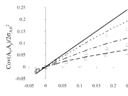
mates is shown in Figure 2 for a range of␣Ofixandh20, through full-sib mating alone, although sinceNS ⫽ND

there were no half-sibs. For the lower extreme shown along with the respective neutral expectation under ran-dom selection (i.e.,h2

0⫽0). The values shown in Figure in Figure 1, with␣Ofix⫽0,φobswas⬎0 althoughφexp⫽

0. This should be expected for two reasons: in a small 2 are1_⁄

2cov(Ai,Aj)/␴2A,0, since they have an expectation population the probability of a full-sib mating is not

Figure2.—Relationship between the covariance between Figure1.—Relationship between the proportion of full-sib

matings (φ) and the initial heritability (h2

0), for phenotypic the breeding values of mates (cov(Ai,Aj)), scaled by 2␴2A,0, and

␣Ofix, for phenotypic selection with different initial

heritabili-selection with different values of␣Ofix. The lines are predicted

relationships usingφ⫽4␣Ofix/(1⫹3␣Ofix), and the points are ties (h20). The lines are predicted relationships using Equation

4, and the points are observations from simulated populations observations from simulated populations (N⫽32,nO⫽16).

Predictions are: zero with␣Ofix⫽0; - - -,␣Ofix⫽0.24; – –,␣Ofix⫽ (N ⫽ 32,nO⫽ 4). Predictions are: —,h20⫽0 (neutral

the-ory); - - -,h2

0⫽0.05; – - –,h20⫽0.2; – –,h20⫽0.4. Simulations

0.06. Simulations are: 䊊, ␣Ofix ⫽ 0.24; 䊐, ␣Ofix ⫽ 0.06; 䉫,

Figure3.—Relationship between equilibrium genetic

vari-Figure4.—Relationship between␤and␣Ofix, for phenotypic

ance prior to selection within a generation (␴2

A), scaled by

selection with different initial heritabilities (h2

0) and family

␴2

A,0, and␣Ofix, for phenotypic selection with different initial

sizes (nO). The lines are observations from simulated

popula-heritabilities (h2

0). The lines are predicted relationships using

tions (N⫽32), where䊏with thick lines arenO⫽16;䊐with

Equation 5, and the points are observations from simulated

thin lines,nO⫽4; —,h20⫽0.01; – –,h20⫽0.2; - - -,h20⫽0.4.

populations (N ⫽ 32, nO ⫽ 4). Predictions are: —, h20⫽ 0

(neutral theory); - - -,h2

0⫽0.05; – - –,h20⫽0.2; – –,h20⫽0.4.

Simulations are:䊊,h2

0⫽0.05;⌬,h20⫽0.2;䊐,h20⫽0.4.

ships of ␤ with h2

0 and nOare fully consistent with the findings ofWoolliamset al. (1999) for random mating. It may be expected from neutral theory that increas-of␣Ofixfor neutral theory. The clear result is that

direc-ing ␣O would increase the regression on the selective tional selection reduces the covariance of mates from

advantage since selected offspring will be more likely what is expected under neutral theory. Furthermore,

to be mated to relatives, so reinforcing the strength or this reduction is well predicted using Equation 4 andφ⫽

weakness of the inherited selective advantage,i.e., the 4␣/(1⫹3␣) (with␣replaced by␣Ofix). In the examples

mean parental breeding value, not only predicts the shown in Figure 2, the covariance among mates remains

breeding value of its offspring but also predicts that of approximately linearly related to ␣Ofix, but the slope _{its offspring’s mate. This is clearly the case for low}

h2 0: of this relationship becomes lower as the heritability

for example, forh2

0⫽0.01 andnO⫽16, as␣Ofixincreased increased from 0 to 0.4. The application of Equation 4

from 0 to 0.24, ␤ increased more than threefold in a withbaf ⫽0 also results in a lower covariance than that _{linear relationship with} ␣

Ofix. However ash20 increased, expected from neutral theory, but results in

overesti-the slope of this relationship with␣Ofixwas substantially mates of the covariance; e.g., for h2

0⫽0.40 and ␣Ofix ⫽ _{lower. Forn}

O⫽16 andh20⫽0.99, no increase in␤with 0.18, the observed scaled value was 0.050, and Equation _␣

Ofixwas observed (result not shown). This reduction in 4 predicts 0.082 and 0.057 with and without settingbaf⫽ _{the slope of the relationship between}␤_and␣

Ofixis

di-0, respectively. _{rectly related to the phenomenon displayed in Figure}

Given that the genetic covariance among mates con- _{2 concerning the covariance between mates as described} tributes to the genetic variance under nonrandom mat- _{above: when ␣}

Ofix and h20 are large, the covariance is ing, a reduction in the former component from that _{lower than that expected from neutral theory and the} predicted by neutral theory will potentially result in a _{selective advantage is poorer than expected at} pre-reduction in the latter. This is confirmed in Figure 3 _{dicting the selective advantage of the offspring’s mate.} with stochastic simulations and predictions using Equa- _{The impact of the nonrandom mating on the} ex-tion 5. With selecex-tion, the genetic variance in the popu- _{pected gene flows conditional on the selective} advan-lation can belowerwith␣Ofix⬎0 than when comparable _{tage (i.e., the sum of the breeding values of an individual} selection is practiced in randomly mated populations. _{and its mate) is shown in Figure 5, measured by the CV} The predictions from Equation 5 tend to overpredict _{of␮k(see Equation 10). The values presented in Figure} the genetic variance by more than is expected from _{5 use parameters in Equation 10 estimated from the} reductions due to finite sample size alone. _{simulations. For␣Ofix⫽ 0, it is clear that the impact of}

Effects of nonrandom mating on the expected gene _{the selective advantage on gene flow is greatest when} flow:Figure 4 shows the relationship between the regres- 0.4 ⬍ h2

0 ⬍ 0.6, with close to 4-fold impact compared sion coefficient of long-term genetic contributions on to h2

0 ⫽0.01. The impact of the selective advantage is the sum of selective advantages of mating pairs and␣Ofix. increased when␣Ofixincreases, but is more sensitive to For a given␣Ofix, for all combinations ofh20andnOstud- changes in␣Ofixwhenh20is low. Therefore, when␣Ofix⫽ ied, ␤ increased asnOincreased (and hence selection 0.24, the maximum impact is close to h20 ⫽ 0.2 and is

only 1.5-fold greater compared toh2

0 ⫽0.01. intensity) and decreased ash2

relation-Figure5.—Relationship between CV of expected long-term genetic contributions [CV(␮k)] and initial heritability (h20), for

Figure 6.—Relationship between asymptotic rate of in-phenotypic selection with different values of␣Ofix. The lines

breeding (⌬F) and initial heritability (h2

0), for phenotypic

se-are modeled using Equation 10 with parameters estimated

lection with different values of␣Ofix. The lines are predicted

from the simulations (N⫽32,nO⫽16). The different lines

relationships using Equation 6, and the points are observations are:䊐, ␣Ofix⫽ 0.24;⌬, ␣Ofix⫽ 0.06;䊊, ␣Ofix ⫽0; 䉫, ␣Ofix⫽

from simulated populations (N⫽32, nO⫽16). Predictions

⫺0.03.

are: —,␣Ofix⫽0.24; – –,␣Ofix⫽0.06; - - -,␣Ofix⫽0; – - –,␣Ofix⫽

⫺0.03. Simulations are: 䊐, ␣Ofix ⫽ 0.24; ⌬, ␣Ofix ⫽ 0.06; 䊊,

␣Ofix⫽0;䉫,␣Ofix⫽ ⫺0.03.

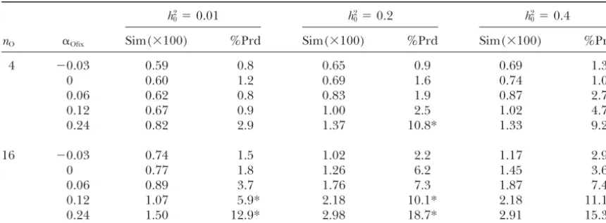
Effect of nonrandom mating on predictions of ⌬F

and⌬Gbased on long-term genetic contributions:The effect of nonrandom mating on⌬Fis shown in Figure

showed that extrapolating expectations of genetic vari-6 and Table 2 contrasts predictions using Equation vari-6

ance and covariance among mates for a neutral trait for two different selection intensities. The pattern of

with nonrandom mating can be qualitatively wrong, with relationship between⌬Fandh2

0and␣Ofixis very similar

deviations toward severe overprediction. Deviations to Figure 5, in that theh2

0with the maximum⌬Fbecomes

were largest when heritability and selection intensity lower as ␣Ofix increases, and ⌬F increases very rapidly

were large and there was a strong preferential mating of for smallh2

0when␣Ofixis large.

relatives. While nonrandom mating had a considerable Predictions of⌬Fusing Equation 6 always

underesti-effect upon the impact of selective advantage for low mated the observed⌬F, but this is expected by a fraction

heritability, as measured by the regression of genetic approximately equal to 2⌬F (Woolliams and Bijma

contributions on the selective advantage and the CV of 2000). When this is accounted for (as in Table 2), the

the expected gene flow conditional on the selective serious errors occur only when selection intensity and

advantage, the phenomenon described by the model

␣Ofixare high. The pattern of these errors is similar to

substantially reduces this effect for moderate heritabili-the cases in Table 1, where ␣Ic and ␣Ir show serious

ties. Furthermore, the study showed that high selection discrepancies. The predictions shown use␣Ir in

Equa-intensity can induce a negative covariance between the tion 6, and not ␣Ic, since ␣Ir provided more reliable

long-term genetic contribution of an ancestor and its predictions than ␣Ic. Where serious discrepancies

oc-␣I, particularly when ␣O is large, and suggested that curred between the observed⌬Fand⌬Fpredicted from

selection acts to attenuate the strong preferential mat-Equation 6, the prediction error could be approximately

ing of relatives. halved (results not shown) by modifying Equation 6 to

A logical starting point for interpreting the results be ⌬F⫽ 1_⁄

4兺kr2k(1 ⫺ ␣I(k)), so that each individual’s

of deviations from neutral expectations is the genetic squared contribution was scaled by the individual’s own

covariance achieved among mates for a selected trait

␣I. This partially overcame the covariance that was

de-when nonrandom mating was practiced. Naively, the scribed above betweenrkand␣I(k). Finally, predictions

preferential mating of relatives would be expected to of⌬G(not shown) obtained from Equation 7 were

accu-result in a clear positive genetic covariance among rate for most of the assessed cases, and often their errors

breeding values, since for a neutral trait this covariance were⬍5% within the range of parametric settings

inves-has an expectation equal to 2␣O␴2A,0 (e.g., Caballero tigated.

andHill1992), and this is also shown in our simulations for neutral traits, so provides a methodological valida-DISCUSSION

tion for our study. However, the predictive model for the covariance among mates showed that inducing such This article has provided a novel model for predicting

a covariance by using pedigree information during se-the impact of nonrandom mating on se-the covariance

lection will lead to a covariance of opposite sign between among mates of populations undergoing selection.

Men-TABLE 2

Simulatedvs.predicted rates of inbreeding

h2

0⫽0.01 h20⫽0.2 h20⫽0.4

nO ␣Ofix Sim(⫻100) %Prd Sim(⫻100) %Prd Sim(⫻100) %Prd

4 ⫺0.03 0.59 0.8 0.65 0.9 0.69 1.3

0 0.60 1.2 0.69 1.6 0.74 1.0

0.06 0.62 0.8 0.83 1.9 0.87 2.7

0.12 0.67 0.9 1.00 2.5 1.02 4.7

0.24 0.82 2.9 1.37 10.8* 1.33 9.2*

16 ⫺0.03 0.74 1.5 1.02 2.2 1.17 2.9

0 0.77 1.8 1.26 6.2 1.45 3.6

0.06 0.89 3.7 1.76 7.3 1.87 7.4

0.12 1.07 5.9* 2.18 10.1* 2.18 11.1*

0.24 1.50 12.9* 2.98 18.7* 2.91 15.3*

Simulated (Sim) rate of inbreeding (⫻100), together with prediction errors from using Equation 6, for phenotypic selection andN⫽32, different target departures from Hardy-Weinberg proportions (␣Ofix), family

sizes (nO), and heritabilities (h20) is shown. * indicates when the difference was⬎(5⌬F)⫻100. Standard errors

of Sim(⫻100) were ⬍0.01, except for␣Ofix ⫽0.24 where the standard errors were ⬍0.03. Prediction errors

are expressed as a percentage of deviation (%Prd) ⫽ 100⫻ ([Sim ⫺ Prd]/Sim), where Prd comes from Equation 6.

delian sampling term of its mate. Therefore when there it cannot cope with nonrandomness coming from other sources such as preference/avoidance of half-sibs and is a preferential mating, or avoidance, of relatives the

induced covariance is offset by this opposing covariance, (ii) the predictions provided by Ghai while broadly reli-able were not without error. In the model, Ghai’s for-which can be substantial. This is in addition to another

opposing effect that is directly analogous to Bulmer mula was used to translate the desired␣Oto an expected covariance among the true family means of mates in the (1980) by which the change in the Mendelian sampling

variance with␣Ihas an impact on the replenishment of selected population; consequently, some improvement might arise from a more general approach to this rela-the genetic variation that is lost through selection in

each generation. tionship.

The reduction in covariance between mates arising The mechanism underlying this model was

potenti-ated as the intensity of selection increased and as the with selection has direct consequences for the additive genetic variance and for the relationship between long-heritability increased. In this article where the results

presented have been concerned with selection upon term genetic contributions and the selective advantage. Both are reduced below expectations based upon neu-phenotype, the heritability represented the squared

ac-curacy of selection and, together with the value of␣I, tral theory. The impact on genetic variance is sufficient for the equilibrium genetic variance (i.e., where Mende-determined the split in information between the

pedi-gree and the Mendelian sampling term (important in lian sampling variance is not reduced each generation as inbreeding progresses) to be less for preferential Equations 2, 3, and 5). In more general selection

schemes the power of the mechanism would depend mating of relatives than for random mating whenh2 0 is high, a qualitative difference. The regression of the on the balance of pedigree information on a candidate

and information on its Mendelian components and the long-term genetic contribution on the sum of the ances-tral breeding value and the average of its mates would use made of such information (e.g., within-family

selec-tion should not generate such a mechanism), rather also be expected to increase under neutral theory, since this has a covariance not only with the offspring’s breed-than on the accuracy alone.

While the model provides an explanation of some ing value but also with that of the offspring’s mate. Note that this expectation arises from the nonrandom mating of the results, it has some limitations. First, while its

predictions are more credible than those based on neu- in the offspring generation, not the ancestors: in the ancestor’s generation the nonrandom mating is fully tral theory, the precision leaves some scope for believing

that other mechanisms may be operating. Of greater accounted for by regression on both parents. However, if the covariance between mates is reduced then so is the significance is that the covariance between mates is

esti-mated by assuming that the proportion of full-sib mating predictive value of the ancestor’s selective advantages. The impact of h2

0 on the CV of the expected gene was that predicted byGhai’s (1969) formula. The use

of this formula has two problems: (i) it is limited to flow is similar to the impact of h2

0 on ⌬F that was ob-served in this study and that of Santiagoand

Caballero, A., E. SantiagoandM. A. Toro, 1996 Systems of

mat-lero (1995). This relationship shows a much greater

ing to reduce inbreeding in selected populations. Anim. Sci.62:

sensitivity to nonrandom mating when the heritability _431–442.

Cockerham, C. C., 1967 Group inbreeding and coancestry. Genetics

is low than when it is either moderate or high. This can

56:89–104.

be explained by the behavior of the covariance between

Ferna´ndez, J., and M. A. Toro, 1999 The use of mathematical

mates and its separate consequences for ␤ and ␴2

A as programming to control inbreeding in selection schemes. J. Anim. Breed. Genet.116:447–466.

described, since changes in both parameters are

respon-Frankham, R., J. D. BallouandD. A. Briscoe, 2002 Introduction

sive to changes with␣Iwhen the heritability is low, but

to Conservation Genetics. Cambridge University Press, Cambridge,

decrease in sensitivity as heritability increases. The simi- _UK.

Ghai, G. L., 1969 Structure of population under mixed random

larity between CV(␮k) and⌬Fin their relationship with

and sib mating. Theor. Appl. Genet.39:179–182.

␣Imay be anticipated since in Equation 6, which relates

Grundy, B., B. VillanuevaandJ. A. Woolliams, 1998 Dynamic

⌬Fto squared contributions, the termE[兺r2

k] is equiva- _{selection procedures for constrained inbreeding and their}

conse-quences for pedigree development. Genet. Res.72:159–168.

lent to E[兺(␮2

k⫹ ␴2k)], where ␮kand ␴2k are the mean

Klieve, H. M., B. P. KinghornandS. A. Barwick, 1994 The joint

and variance of the contributions conditional upon the

regulation of genetic gain and inbreeding under mate selection.

selective advantages. Woolliams and Bijma (2000) _{J. Anim. Breed. Genet.111:81–88.}

Lynch, M., andB. Walsh, 1998 Genetics and Analysis of Quantitative

showed that␴2

k⬇␮2kfor random mating, but an

analo-Traits. Sinauer Associates, Sunderland, MA.

gous relationship has not been established for

nonran-Meuwissen, T. H. E., 1997 Maximizing response of selection with

dom mating, although it has been established that␴2

k _{a predefined rate of inbreeding. J. Anim. Sci.75:934–940.}

Press, W. H., S. A.Teukolsky, W. T.Vetterlingand B. P.Flannery,

will depend upon␣I: avoidance of relatives reduces␴2k

1992 Numerical Recipes in FORTRAN: The Art of Scientific

Comput-(e.g.,Wang1997), whereas preferential mating of

rela-ing. Cambridge University Press, Cambridge, UK.

tives increases␴2

k (e.g.,CaballeroandHill1992). _{Robertson, A., 1965 The interpretation of genotypic ratios in}

do-mestic animal populations. Anim. Prod.7:319–324.

In conclusion, this study has described mechanisms

Sa´nchez, L., C. Garcı´aandM. A. Toro, 1999 Improving the

selec-that influence the covariance observed between mates

tion efficiency of artificial selection: more selection pressure with

for a trait that is subject to selection when mating is _{less inbreeding. Genetics151:1103–1114.}

Sa´nchez, L., P. BijmaandJ. A. Woolliams, 2003 Minimizing

in-nonrandom. In particular, the covariance is

substan-breeding by managing genetic contributions across generations.

tially less than that expected from neutral theory, partic- _Genetics

164:1589–1598.

ularly when the heritability is moderate or high, and Santiago, E., andA. Caballero, 1995 Effective size in population under selection. Genetics139:1013–1030.

this has consequences for the observed additive genetic

Sonesson, A. K., andT. H. E. Meuwissen, 2000 Mating schemes

variance, the scale of expected gene flow that is directly

for optimum contribution selection with constrained rates of

attributable to the selective advantage, and⌬F. The ob- inbreeding. Genet. Sel. Evol.32:231–248.

Toro, M. A., andM. Pe´rez-Enciso, 1990 Optimization of selection

served sensitivity to nonrandom mating of the latter two

response under restricted inbreeding. Genet. Sel. Evol.22:93–

phenomena when heritability is low can be explained _107.

with reference to neutral theory, and the study shows Wang, J., 1996 Deviation from Hardy-Weinberg proportions in finite populations. Genet. Res.68:249–257.

that it is the lack of sensitivity for moderate to high

Wang, J., 1997 More efficient breeding systems for controlling

in-heritabilities that required the development of theory. _{breeding and effective size in animal populations. Heredity79:}

591–599. We are grateful to two anonymous referees whose careful reading

Woolliams, J. A., 1989 Modifications to MOET nucleus breeding and constructive suggestions greatly improved all aspects of this

manu-schemes to improve rates of genetic progress and decrease rates script. The authors gratefully acknowledge support from the

Euro-of inbreeding in dairy cattle. Anim. Prod.48:31–35.

pean Commission in the form of a Marie Curie Fellowship (L.S.) and _{Woolliams, J. A., andP. Bijma, 2000 Predicting rates of inbreeding} from the Department for the Environment, Food, and Rural Affairs _{in populations undergoing selection. Genetics154:1851–1864.} in the United Kingdom ( J.A.W.). Woolliams, J. A., P. BijmaandB. Villanueva, 1999 Expected ge-netic contributions and their impact on gene flow and gege-netic gain. Genetics153:1009–1020.

Wray, N. R., andM. E. Goddard, 1994 Increasing long-term re-sponse to selection. Genet. Sel. Evol.26:431–451.

LITERATURE CITED

Wright, S., 1969 The Theory of Gene Frequencies(Evolution and the

Bulmer, M. G., 1980 The Mathematical Theory of Quantitative Genetics. _{Genetics of Populations, Vol. 2). The University of Chicago Press,}

Clarendon Press, Oxford. _Chicago.

Caballero, A., andW. G. Hill, 1992 Effective size of non-random