ABSTRACT
RHOULAC, TORI DANIELLE. School Transportation Mode Choice and Potential Impacts of Automated Vehicle Location Technology. (Nagui M. Rouphail, Advisor)
School-related traffic congestion is a large problem in North Carolina and throughout the nation. North Carolina Department of Transportation works with schools and municipalities to better design and retrofit campuses to accommodate the vehicular volumes that often queue onto adjacent streets and cause long delays. The large number of school trips made by automobile not only cause traffic problems, but safety problems as well, made evident by injury and fatality statistics. The goal of this research was to ultimately enhance student safety and reduce school-related traffic problems by gaining a better understanding of the household attributes and behaviors that influence school transportation mode choice in order to identify problems and prioritize solutions for school transportation, including school bus service improvements through automated vehicle location (AVL).
SCHOOL TRANSPORTATION MODE CHOICE
AND POTENTIAL IMPACTS OF AUTOMATED VEHICLE LOCATION TECHNOLOGY
by
TORI D. RHOULAC
A Dissertation Submitted to the Graduate Faculty of North Carolina State University In Partial Fulfillment of the Requirements for the Degree of
Doctor of Philosophy
Department of Civil Engineering Raleigh, NC
June 2003
Approved by:
___________________________________ Dr. Nagui M. Rouphail
Chair of Advisory Committee
___________________________________ ___________________________________ Dr. Joseph E. Hummer Dr. John R. Stone
BIOGRAPHY
TORI DANIELLE RHOULAC is a native of Hampton, Virginia. She was educated in the Hampton City Public Schools and graduated from Kecoughtan High School in June 1994. Her undergraduate education was completed at Howard University in Washington, District of Columbia, where she earned a Bachelor of Science degree in Civil Engineering with a concentration in Transportation. In May 1998, she began her studies at North
Carolina State University in Raleigh, North Carolina, earning a Master of Science degree in Civil Engineering with a focus on Transportation Systems in August 2000. She will
complete degree requirements for the Doctor of Philosophy in Civil Engineering in the summer of 2003.
ACKNOWLEDGEMENTS
To my Lord and Savior, Jesus Christ, thank You for guiding me, making provisions, and bringing me to this “wealthy place.”
To my family and friends, thank you for your constant love and undying support.
To my advisor, Dr. Nagui Rouphail- Professor of Civil Engineering and the members of my advisory committee: Dr. Joe Hummer- Associate Professor of Civil Engineering, Dr. John Monahan- Professor of Statistics, and Dr. John Stone, Associate Professor of Civil
Engineering, thank you for giving of your time and talents to make this academic achievement possible for me.
To Jeff Tsai- Director of the Pupil Transportation Group at the Institute for Transportation Research and Education (ITRE), whose vision and innovation began this school
transportation research, I say a special “Thank You!”
TABLE OF CONTENTS
Page
LIST OF TABLES vi
LIST OF FIGURES viii
1. INTRODUCTION 1
1.1 Problem Definition 1
1.2 Research Objectives and Scope 4
1.3 Dissertation Organization 7
2. DECISION ANALYSIS AND MODE CHOICE: A LITERATURE REVIEW 9
2.1 Introduction 9
2.2 Mode Choice Concepts 11
2.3 Utility as a Decision Rule in Mode Choice 12
2.4 Probability Unit Models 21
2.5 Data Collection Methodology 24
2.6 Literature Summary 25
3. PRELIMINARY DATA COLLECTION AND ANALYSIS 27
3.1 Introduction 27
3.2 Determining Sample Size 28
3.3 Sample Selection 29
3.4 Survey Results 30
3.5 Spatial Analysis 41
3.6 Survey Error 43
3.7 Preliminary Survey Summary 45
4. MODEL DEVELOPMENT AND CALIBRATION 47
4.1 New Survey Structure 47
4.2 New Survey Error 50
4.3 New Survey Analysis 53
4.4 New Survey Summary and Variable Definition 58
4.5 Model Development 61
4.6 Sensitivity Analysis 79
5. MODEL VALIDATION 83
5.1 Initial Validation Results 83
5.2 Additional Validity Tests 85
6. MODEL IMPACTS AND APPLICATION 88
TABLE OF CONTENTS continued
Page
6.2 Model Application to Individual Schools 93 6.3 Potential Impacts of Automated Vehicle Location 95
6.4 Model Application Using NCWISE 103
7. SUMMARY, CONCLUSIONS, AND RECOMMENDATIONS 105
7.1 Research Summary 105
7.2 Conclusions 108
7.3 Recommendations for Future Research 113
____________
REFERENCES 116
APPENDIX A 120
Preliminary Survey Form APPENDIX B
LIST OF TABLES
Page
Table 3.1 Survey Sample Response Rates by Student Grade Level 31 Table 3.2 Mode Choice by Student Grade Level 33
Table 3.3 High School Mode Choice 33
Table 3.4 Reasons Parents Choose Not to Use the School Bus Service 34 Table 3.5 Profile of Student Characteristics by Mode 41 Table 3.6 Survey Responses by School Bus Ridership Status 45 Table 4.1 New Survey Response Comparison with Overall Student Population 51 Table 4.2 School Transportation Mode Choice Variables 59 Table 4.3 Automobile Convenience Factor Definition 59 Table 4.4 School Bus Convenience Factor Definition 60 Table 4.5 Mode Choice by Perceived Home-to-School Distance 63 Table 4.6 Mode Choice Variable Means by Gender 64 Table 4.7 Income and Convenience Correlations 68
Table 4.8 AM Mode Choice Model Options 69
Table 4.9 PM Mode Choice Model Options 69
Table 4.10 Linear School Transportation Mode Choice Models’ Standard Errors 71
Table 4.11 Logistic School Transportation Mode Choice Models’ Standard Errors 73 Table 4.12 Brier Scores for School Transportation Mode Choice Model 75
Alternatives
Table 5.1 Model Validation Summary 84
LIST OF TABLES continued
Page
Table 5.4 School Transportation Mode Choice Model Results Applied to 86 Second Calibration Data Set
Table 6.1 Wake and Union Counties’ Comparison of Demographic Parameters 90 Table 6.2 Union County Data and Validation Data Comparison 92 Table 6.3a School Transportation Mode Choice Analysis by School: 94
Automobile Probabilities
Table 6.3b School Transportation Mode Choice Analysis by School: 94 Confidence Intervals
Table 6.4 Technology Probabilities for Students “Eligible” for a Modal Shift 100 to the School Bus
LIST OF FIGURES
Page
Figure 1.1 Percentage of Student Population Transported at Public Expense 3 in the U.S.
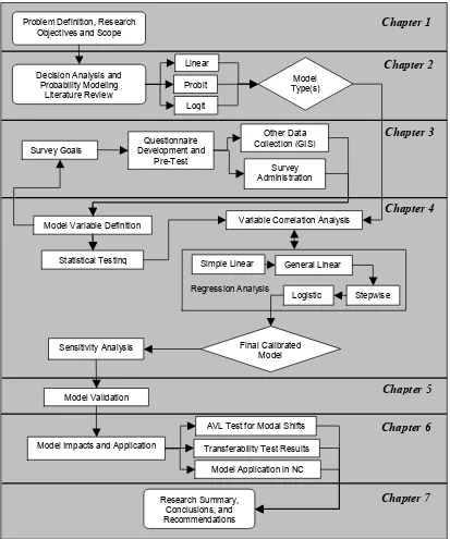
Figure 2.1 Research Methodology 26
Figure 3.1 Distribution of Total Survey Responses by Student Age 32 Figure 3.2 Parental Safety Rating of Two Primary School Transportation Modes 37 Figure 3.3 Parental Assessment of School Bus Punctuality 40 Figure 3.4 Survey Responses on Willingness-to-Pay for Monthly Subscription 40
to AVL Rider Notification Service
Figure 3.5 Survey Responses on Willingness-to-Pay for AVL School 41 Bus Tracking
Figure 4.1 New Survey Responses by Student Grade Level 52 Figure 4.2 Student Transportation Zones 54 Figure 4.3 New Survey K-8 AM Modal Split 57 Figure 4.4 New Survey K-8 PM Modal Split 58 Figure 4.5 Automobile Probabilities for School Trips versus Income 69 Figure 4.6 Logistic Model Calculations 72 Figure 4.7 Model-Forecasted AM and PM Automobile Probabilities 78 Figure 4.8 Variation in AM Automobile Probability by K8HH 80
and Student Grade
Figure 4.9 Variation in AM Automobile Probability by K8HH 81 and Safe Mode Rating
LIST OF FIGURES continued
Page
Figure 4.11 Variation in AM Automobile Probability by K8HH 82 and School Bus Convenience
1. INTRODUCTION
1.1 Problem Definition
traffic. The year 2002 began with a backlog of over 50 requests for similar services at other schools.
The Municipal and School Transportation Assistance Group also assisted with a school campus circulation study in 2002 where student loading/ unloading procedures and vehicle queuing patterns were observed at 20 schools in eight North Carolina counties. Thorough data collection efforts produced results that further substantiate the impact of school trips on traffic patterns. About 50% of the schools involved in the study experienced queues in the afternoon that exceeded their on-campus vehicle storage space causing spillback onto the adjacent street; many of these queues began prior to the time that the bell rang to release students from school (STG 2003). A subsequent impact of such recurring traffic congestion is the disruption to normal traffic patterns that becomes necessary to install turn lanes or widen roads in an attempt to enhance mobility in areas adjacent to schools.
“Nationwide, there appears to be a systemic modal shift from school transportation modes that are relatively safe to modes that are causing operational and safety problems in and around school areas (UNC 2003).” The National Center for Education Statistics (NCES) reports a generally increasing trend in the number of public school students “transported at public expense” in the U.S. from 1929 to 1990. This does not include walkers, bikers, or those students whose school transportation is funded directly by a parent or guardian. Since 1990, however, a decreasing trend has been observed. Figure 1.1 displays these trends, charting the percentage of the total student population transported by school bus for each school year since 1929. Perhaps, the decreasing trend since 1990 is due to families now choosing the most convenient mode for parents and students.
0 10 20 30 40 50 60 70
1920 1930 1940 1950 1960 1970 1980 1990 2000
Figure 1.1 Percentage of Student Population Transported At Public Expense in the U.S. (NCES 1998)
common technology used in trucking and busing systems to increase ridership and improve safety and efficiency. Similar AVL systems may prove to be beneficial for school bus systems. Through AVL, the location of each vehicle in a fleet can be tracked using Global Positioning System (GPS) receivers. Software supplements to AVL display the vehicle position on computerized maps of the area allowing for real-time information gathering, dissemination of vehicle arrival times, and quicker emergency response. Several AVL systems have been created specifically for school bus systems to provide the safety and operational benefits of tracking. Mode choice data are needed, however, to determine the potential “market,” if any, for these potential improvements through AVL. “Parents and students often do not consider the associated risks [of a travel mode] and choose or encourage the use of school travel modes for reasons apart from maximizing safety or minimizing risk [like] convenience, flexibility, or cost savings (Fischbeck 2003).” AVL systems not only provide safety benefits, however, traveler convenience may also be increased.
1.2 Research Objectives and Scope
Based on the need to better understand the behaviors and decisions involved in school transportation mode choice, the following research objectives were developed:
1. To develop, calibrate, and validate a school transportation mode choice model for a selected school district.
The factors that contribute to school transportation mode choice were analyzed using mathematical and transportation modeling techniques. The analysis included an assessment of “customer service,” which is parental perception of school bus system performance and “transportation service,” which is the school bus level of service compared with other modes. Not all school transportation modes were included in the analysis. A reduced set of three modal alternatives was considered: nonmotorized, comprised of bicycle and pedestrian modes, school bus, and automobile. This decision was made primarily because of small sample sizes for the other modal alternatives.
Public school students in grades K – 12 were the focus for data collection. Private school policies differ concerning the provision of bus transportation, making the available modes vary by school. So, private schools were not included in this analysis, nor were preschool students, whose available modes also differ, based on the program in which they enrolled. No activity bus trips for student field trips or athletic events were considered in this analysis. The focus was school trips during the “normal school transportation hours” of 6 – 9am and 2 – 5pm, Monday through Friday, late August through mid June.
The survey collected data on mode choice for individual students, although the impact of other students in the household was considered. Discussion of travel time, wait time, or other similar concepts refer to that of the student. Some parents walk with their children to school or wait with their children at the bus stop; others do not. Some parents drive their children to school as part of a trip chain; others drive round-trip from the school to the home. There is large variability in parent behavior related to school travel and therefore student trips, not parent trips, were the focus of the analysis.
Both linear and logistic probability models were considered for mode choice model development with utility theory as the basis. The term, “likelihood,” is sometimes used interchangeably with “probability” in explaining results.
The final models are expected to be applicable in any North Carolina county. While data were collected in only one county, results from a test for transferability in another county with quite different characteristics suggest that the models are transferable to any area where the approximate automobile usage falls within a certain range in the morning and afternoon.
Ultimately, this research should increase school transportation safety and complement school planning studies throughout the state by providing a means of estimating school transportation modal shares based on certain characteristics of the student population. Further cultivation of a productive and harmonious relationship between school transportation and transportation engineering methodologies is also desired.
1.3 Dissertation Organization
This study of school transportation mode choice was undertaken using a combination of research methodologies. A description of the problem has been included in this
introductory chapter, along with a definition of the research objectives and scope. The literature review of pertinent decision analysis, mode choice and probability modeling theories and methods follows in Chapter 2. Linear, logit, and probit probability models were reviewed.
individual student information. Transportation system performance data are often collected through demonstration projects, but this was not feasible for the AVL component due to financial constraints, so surveying was used to collect AVL data as well. Chapters 3 and 4 document the data collection methodologies and analyses for the two surveys incorporated in this research project. Chapters 4 and 5 detail the model development, calibration, and validation processes. The AVL technology assessment uses standard mathematical methods to evaluate the potential for modal shifts to the school bus due to technological
2. DECISION ANALYSIS AND MODE CHOICE: A LITERATURE REVIEW
2.1 Introduction
The theory of decision analysis is based on the need to consider and evaluate complex decisions amongst alternatives that differ significantly. Formal analysis of a decision, or a set of decisions, typically becomes necessary when a problem has a large number of factors or involves multiple decision makers or uncertainty. This type of analysis is not only common in business, social science, and operations research, but also in transportation. Decision analysis is used regularly in transportation planning to model a traveler’s choice of destination, mode, and route.
choices of destination are analyzed and a specific point of origin and destination are assigned to each trip. Mode choice forecasts the distribution of trips among the available modes. This is the analysis of traveler choice of mode. In small cities and regions where public transportation is not provided, the mode choice step is often omitted because automobile travel is assumed for everyone. The final step, network assignment, assigns trips to specific routes in the network based on analysis of traveler choice of route. Automobile trips, for example, are assigned to the highway network of streets and freeways.
When modeling any choice, there are four fundamental issues that should be considered: the characteristics of the decision maker, the available alternatives, the attributes of the alternatives, and the decision rules that will be used in analysis (Ben-Akiva 1985). The decision maker can be an individual or a group as is the case in household decision making. The list of alternatives may comprise the universal set of alternatives for the decision being analyzed or the reduced set of alternatives available to a particular individual or group. Specified attributes are those characteristics of each alternative that differ greatly and affect choice. Finally, the decision rules are the standards used by the decision maker to select an alternative.
2.2 Mode Choice Concepts
“Preferences among a set of options depend on the attributes of the options and of the individual involved (Horowitz 1986).” Therefore, a mode choice model of traveler preferences will include terms describing attributes of the individual making the decision, the trip purpose, and the mode, typically characterized by cost and level of service. Mode choice models do not include trip type when the research focus is a single trip purpose. School transportation research is one example, considering only home-based school trips.
School and work trips are known to behave similarly. “Work trips are undertaken with daily regularity, mostly during the morning and afternoon period of peak traffic, and overwhelmingly from the same origins to the same destinations. This is also true in the case of school trips (Papacostas 2001).” Many of the observations and theories of home-based work travel can therefore be applied to home-based school travel. Another similarity between these two trip types is the set of competing modes. In a typical transportation region, automobile and transit trips comprise the overwhelming demand placed on the transportation network. Pedestrian and bicycle modes are more popular in the urban core and areas near colleges and universities. Available school transportation modes are
automobile, school bus (a form of transit), walking, biking, contracted van service, or public transit. There are sets of students whose choices are limited because they live in an area where school bus service is not provided or because their family does not own an
automobile. These special groups are discussed in more detail in Section 4.3.
of transit that have been the focus of research efforts for decades. Individual characteristics, such as socioeconomic status, play an important role in the sensitivity of the mode choice decision to cost and preference.
2.3 Utility as a Decision Rule in Mode Choice
Utility is the decision rule used to analyze mode choice, providing “a numeric measure of attractiveness (Hunt 1990).” Disutility measures the cost, or unattractiveness, associated with a particular mode. Models of choice among modal alternatives generally attempt to maximize utility or minimize disutility by comparing (dis)utility among the available modes.
Disutility is a function of three primary considerations- out-of-pocket costs, travel time, and convenience- which are measured by a variety of factors and together make up the relative attractiveness of modal alternatives. Transit research completed at the Center for Urban Transportation Research confirms that schedule flexibility, a measure of convenience, in addition to travel time and out-of-pocket costs are the important contributors to mode choice (Ball 1990).
2.3.1 Socioeconomic Impacts: Costs and Income
1992).” Marginal costs, however, involve only the consumable items used for fuel and maintenance. Drivers rarely, if ever, consider the fixed costs of owning an automobile when making the decision of whether or not to drive an automobile. Therefore, mode choice decisions are based on marginal costs instead of average costs.
Trends in the marginal costs of fuel, oil, and tires can help determine the future attractiveness of the automobile mode. Since the advent of Corporate Average Fuel Economy (CAFE) standards in 1975, fuel economy has increased for passenger cars from approximately 16 miles per gallon in 1980 to almost 22 miles per gallon in 1992 (Allen 1996). Department of Energy projections for the year 2025 exceed 30 miles per gallon (EIA 2003). Conversely, maintenance costs have increased as vehicle technology becomes more complex. Fuel prices fluctuate monthly, but follow an upward, long-term trend. Forecasted energy prices show a constant increase through the year 2025 (EIA 2003). Fuel economy trends favor the automobile, but rising gas and maintenance prices could make transit a more attractive option.
There are no out-of-pocket costs to parents whose children use the school bus service. Costs for operating an automobile are usually negligible, especially for those parents who chain their work trips with school trips. Increasing average home-to-school distances in school districts where magnet and year-round schools are options may make automobile operating costs a more important consideration in the mode choice decision. The out-of-pocket cost for students using public transit equals the fare. Consideration of these monetary factors introduces the importance of socioeconomic factors in mode choice.
automobile and therefore are not considered transit riders by choice. A study by the Center for Urban Transportation Research (CUTR) noted several reasons that travelers with a choice select public transit for work trips into the central city, urban environment. These include cost and availability of parking, followed by traffic congestion and travel times (Ball 1990). Cities with subway systems, where travel times can be drastically reduced because of the exclusive right of way operation, were included in this study. Of the captive transit riders participating in the CUTR survey, about 37% said they would drive if an automobile were available. This means that 63% of captive transit riders would likely continue to use transit, even with an automobile available because of parking costs and availability, travel times, and traffic congestion. This may indicate that socioeconomic factors are not critical in mode choice decisions for many travelers. Further research, however, shows that choice of transit is highly correlated with income. The percentage of persons indicating a willingness to use a paratransit service for transport to work in the same survey decreased steadily from 60% in households with an annual income of less than $10,000 to 40% in households with annual incomes greater than $50,000 (Ball 1990). The potential for prompting school trip modal shifts is also expected to vary with household income.
2.3.2 Travel Time Impacts
to delays caused by traffic congestion, accidents, construction, and other occurrences on the highway system. Transit would have additional utility if exclusive right-of-way were provided. The stops that a bus makes to board or alight passengers cause increased in-vehicle travel times and less than ideal routing for buses.
traffic signals or traffic congestion adds to travel times in urban areas, as opposed to the nearly free-flow traffic conditions encountered in rural regions. School transportation mode choice could therefore vary by area type because of the associated travel time implications.
Bicycle and pedestrian modes have longer “in-vehicle” travel times relative to automobiles because they are non-motorized, but they become more attractive when considering ease of access (out-of-vehicle travel time). The following “hierarchy” of the more prominent modes gives the threshold distances at which each is most attractive. “Walking is usually faster than the car for perhaps some 400 meters (437 yards), depending largely on the time lost getting to and parking the car. Somewhere between 20 and 400 meters the cyclist overtakes the pedestrian, having to overcome the delay of getting to the bicycle and unlocking it. The car and bicycle dominate after some 400 meters… the car overtakes the bike at around 1.5 kilometers (just under a mile), and transit overtakes the pedestrian at a similar distance (Wright 1992).” These distances apply to normal traffic conditions; congestion will make walking and biking more attractive for longer distances.
tend to be more willing to wait or walk longer distances for work trips than for shopping trips (Beimborn 1995).”
2.3.3 Convenience
least safe by about 15% of respondents (Ball 1990). This is another reason that the convenience term for the automobile exceeds all other modes. A mode perceived as safer than others will also be seen as more convenient.
Personal environment control is another convenience factor in favor of the personal automobile. Many travelers enjoy having full control of musical selection during a commute in their personal automobiles. Differing preferences of musical genres keep music from being played on most public transportation modes. Portable music listening devices, like a walkman or discman, however, allow the traveler to be more in control of his or her personal environment on transit trips. Conversely, there are no technologies that allow for personal control of noise level or temperature control in public transportation. There are some personal environment factors that public transportation enhances, like the ability to read during the commute (Wright 1992).
vehicle are not always their personal decisions. Students valuing independence often choose the bike or pedestrian modes, when home-to-school distance permits.
Walking is the least favorable mode when considering ease of carrying things. The list of commonly carried items for students includes lunches, books, book bags, musical instruments, and school projects. Bicycles are more favorable because of baskets and other devices that help to transport large items (Wright 1992). Personal automobiles are most convenient for carrying multiple items because loading and can be completed over a longer period of time, also because there are not usually space constraints. On a bus, however, all the items must be carried at the same time to the bus stop and onto the bus and the space once on board is limited.
2.3.4 The Utility Function
There is a deterministic portion and a probabilistic, or random, portion of the utility on which an individual’s choice of mode is based. The deterministic function is a linear combination of variables that expresses the relative utility of a mode using the general form:
i i i
i i i
i n n
i a a X a X a X
U = 0 + 1 1 + 2 2 +...+ Equation 2.1
where U is the utility for mode i, defined by the attributes, i
X1 through Xni, and weighted by
the coefficients, a1ithrough ani with a0ias the model constant. Utility functions can be
Field data describing trip and decision maker characteristics are necessary to calibrate utility functions. Household or individual traveler surveys are commonly used to obtain the necessary data for utility function calibration. The “weight” assigned to each variable depends heavily on the relative value that decision makers assign to that factor. For example, past research has proven that travelers value out-of-vehicle travel time, which is a common variable in traditional mode choice models, more than in-vehicle travel time; this is expressed mathematically by assigning a larger coefficient, an, to the out-of-vehicle travel
time variable.
As with any mathematical model, there are some limitations to the deterministic utility model. Firstly, deterministic utility functions result in the same value for utility, given the same input parameters, meaning that a user will always choose to maximize utility or minimize disutility. Behavior is probabilistic, however, and sometimes choices are made that cannot be expressed numerically by a quantified utility. This introduces the probabilistic portion of utility theory, the random error term. This term, discussed in more detail in Section 2.4, is added to the deterministic portion of a utility model, acknowledging that aggregate behaviors are not full estimable.
Finally, the weights assigned to the utility model variables are assumed to be constant for a given trip purpose, but within a single purpose are many differences in the value assigned to the various factors. This is a source of error when utility functions are used to estimate modal split, which is described in Section 2.4.
2.4 Probability Unit Models 2.4.1 Model Specifications
When uncertainty is present in decision making, the model used to link alternatives to their consequences upon which choices are based involves an assessment of probability. Probability models attempt to estimate the probability that a given mode will be used by an individual with certain characteristics and preferences, expressed by the utility function. Individuals are studied because individual decisions determine aggregate behaviors, which are generally of interest in transportation modeling (Ben-Akiva 1985). “Measures of aggregate travel, such as bus ridership, are obtained by adding up the choices of individuals (Horowitz 1986).”
There are numerous types of probability models, including binary, multinomial, linear, probit and logit. A probability model is named by a description of the outcome variable or the random error distribution. Binary models, for example, have two possible outcomes, whereas multinomial models involve three or more choices. Linear, probit, and logit models are the most common probability models, each describing a different
The linear probability model assumes that the error term is zero and the probability that an individual will choose a specific mode is based solely on a linear combination of variables expressing utility. In the binary case, where the two available modes are identified as “0” and “1,” the linear combination of variables estimates the probability that mode one will be used. A limitation of the linear probability model is that values which are negative and greater than one can be calculated. Extreme value limits can be implemented since probabilities can range only between zero and one or the negative and greater-than-one values can be used with the other individual values to estimate the aggregate statistics of interest.
The “probit,” or probability unit, model assumes a normal error term distribution. The logit model is an extension of the probit model with a logistic-distributed random error. Logit and probit are “the two most commonly used alternatives to the linear specification of the probability model (Aldrich 1984).” The logistic probability unit, or “logit,” model is the probability model type used most in forecasting mode choice. The logit model is
characterized as “‘probit-like’ but also more convenient analytically” because the logit model has a “closed form” and does not involve the multiple integrals that are encountered in formulating a multinomial probit model (Ben-Akiva 1985).
The basic difference in the probit and logit models is the scale of coefficient
estimates. Logit coefficients are typically 1.8 times the probit coefficients. The theoretical basis for both models is “essentially identical at all but the tails of their respective
utility of the available modes. For the binary case, only the difference in utility is necessary for modeling, as opposed to a unique utility function for each available mode.
Interpretation of linear probability models is most simple, but can be limited when a continuous dependent variable is not involved. Non-linear probability models do not have this limitation and are therefore widely used in social science analyses, where the “attitudes, behaviors, characteristics, decisions, and events [being studied] are measured in … non-continuous ways (Liao 1994).”
The general form of the logit model is:
∑
=
= n
j U U
i
j i
e e p
1
Equation 2.2
where pi is the proportion of users selecting mode i, Ui is the utility of mode i (Equation 2.1)
and n is the total number of available modes. The general form of the probit model is:
)
( i
i U
p =Φ Equation 2.3
where Φ denotes the standardized cumulative normal distribution.
2.4.2 Probability Model Summary
2.5 Data Collection Methodology
“In travel demand analysis… often a single data collection effort is undertaken to serve many purposes. [Information gathered from interviewing] travelers to find out their chosen alternatives and their attributes [can be] used to estimate the parameters of travel demand models as well as to estimate characteristics of the population such as the mean income of transit users or the distribution of auto ownership across households (Ben-Akiva 1985).” Random sample surveys are commonly used to obtain data on public opinions, attitudes, or behaviors. “Surveys are… the primary way to measure attitudes and determine why people act a certain way (Hummer 1994).” Random sampling is necessary to gain responses representative of an entire population. Inferences about a population are not reliable if drawn from a nonrandom sample.
The numerous surveying methods can be classified in two broad categories- questionnaires and interviews. Each category differs in terms of cost, time and staff required, expected nonresponse bias, potential anonymity of respondents, and many other factors. “The choice of survey method depends on the type of questions and the sample anticipated (Hummer 1994).” Researchers should ensure that adequate resources are available for the method selected and minimum sample size required for their respective studies.
2.6 Literature Summary
Figure 2.1 Research Methodology Decision Analysis and
Probability Modeling Literature Review Problem Definition, Research
Objectives and Scope
Survey Goals Development and Questionnaire Pre-Test
Survey Administration
Other Data Collection (GIS)
Model Variable Definition
Statistical Testing
Variable Correlation Analysis
Sensitivity Analysis Final Calibrated Model
Model Impacts and Application
Chapter 1 Research Summary, Conclusions, and Recommendations Chapter 7 Chapter 6 Chapter 5 Model Validation Chapter 4 Chapter 3 Chapter 2 Model Type(s) Linear Probit Logit
Transferability Test Results AVL Test for Modal Shifts
Model Application in NC Simple Linear General Linear
Stepwise Logistic
3. PRELIMINARY DATA COLLECTION AND ANALYSIS
3.1 Introduction
Household surveys were used to collect data for mode choice model development. This chapter details the surveying methods and results of the preliminary survey. Households having one or more children in kindergarten through twelfth grade were asked questions in accordance with three objectives: 1) to collect data on individual student mode choice and the associated student and family characteristics, 2) to assess the parent’s perception of problems associated with the school bus service, and 3) to determine parental acceptance of and willingness-to-pay for AVL technologies that could better the school bus service. The student researcher developed the survey using guidelines from the Manual of Transportation Engineering Studies (Hummer 1994). Budgetary constraints mandated a mail-out-mail-back survey format, instead of a telephone survey. Months of editing, review, and evaluation were completed for the survey draft questionnaire, including review by experienced surveyors and transportation staff in the selected school district and a test survey with about 20 participants. Upon receiving the necessary approvals, surveys were mailed to parents of 5000 students in the Wake County, NC public school system (WCPSS) in October 2001. Parents were given approximately one month to complete and return the surveys by mail, with an early November requested return deadline. The complete survey form is shown in Appendix A.
staff had expressed interest in exploring AVL technologies for their school bus fleet, so the information obtained in the survey would benefit their AVL research efforts, in addition to providing a supplemental means for assessing their school bus system performance.
3.2 Determining Sample Size
Surveys are intended to estimate the true value of one or more population characteristics (ASA 1997). In order to draw inference from a sample that will accurately reflect the population, careful attention must be given to determining the needed sample size.
According to the theory of probability, if the expected value for probability of success in a “yes or no” experiment is p, then the 95% confidence interval for the expected value is:
n p p Z
p± 0.95× (1− ) Equation 3.1
where Z0.95 = 1.96 for a two sided alternative and n = sample size. The error term is denoted
by δ in Equation 3.2. The “yes/no” assessment in the school transportation survey refers to school bus ridership. A 50%-50% split was assumed for survey respondents answering the question of whether or not they ride the school bus because sampling was random and preliminary research showed about a 53% school bus ridership in Wake County. Both p and (1-p) in Equation 3.1 were set equal to 0.50, representing the maximum product. Therefore, even if actual survey responses did not yield a 50/50 split, the error in the estimate would be no greater. Solving for n yields the following equation:
2
9604 . 0
δ
=
Equation 3.2 calculations indicated that in order to achieve a 1% error, a sample size of approximately 9600 was required. A sample size of 385 corresponded to a 5% error. The sample size selected would depend on the maximum acceptable error rate and the expected response rate. Transportation survey response rates vary widely between 20 and 70% (Hummer 1994). Desiring a 40% response rate and an error less than 5%, a sample size of 5000 was selected. If 2000 completed surveys were returned, the associated error would be just over 2%. Having such a large sample size was beneficial because “larger samples are more likely to yield results close to the target population quantity and thus have smaller margins of error than more modest-sized samples (ASA 1998).”
3.3 Sample Selection
Stratified random sampling was used to determine which of the approximately 100,000 students enrolled in WCPSS for the 2001-2002 school year would receive surveys. The population was stratified so that there would be adequate representation in the sample responses from each part of Wake County. The computerized system used across the State of North Carolina for school bus routing and scheduling divides each county into high school attendance boundaries. There are 15 high schools in Wake County, so student names were separated into 15 categories. All elementary and middle schools are assigned to a high school attendance boundary, so with the school codes from the student information database, 15 separate databases were created corresponding to the 15 high school attendance boundaries.
and middle grade levels are known to exhibit somewhat similar ridership patterns, but the availability of driving as a transport mode for high school students likely makes their ridership patterns different. For this reason, data were further stratified as high school (grades 9-12) and non-high school (grades K-8) in each attendance boundary.
A total of 30 strata were used corresponding to the 15 high school attendance boundaries and two grade levels, K-8 and 9-12, in each. Using a random number generator, 167 student names were selected from each of the 30 categories by the corresponding record number. Duplicate addresses were deleted if siblings with the same mailing address were randomly selected. A few of the selected students had incomplete address information; these names were also deleted from the database. After removing the duplicate and incomplete entries, approximately 4980 names remained. Twenty additional students from the alternative high school database were then randomly selected for inclusion in the survey.
In order to achieve anonymity of responses, surveys were not tracked according to the households to which they were sent. Instead, researchers planned to use average distance to school by high school attendance boundary as a surrogate measure for actual home-to-school distance in model development. Ultimately, the distance data collected in the new survey, which is discussed in Chapter 4, were used in model development.
3.4 Survey Results
collected for 2302 students. Using Equation 3.2, a sample size of 2300 corresponds to an expected error of about 2%. Sources of error in surveys and associated measures used to calculate this error are discussed in further detail in Section 3.7.
3.4.1 Student Age, Grade, and Gender
Analysis of survey results revealed that responses by grade level closely matched population grade level proportions. Elementary and middle school students are thought to exhibit similar bus ridership behaviors, unlike high school students. Grouping elementary and middle into a single category, WCPSS is comprised of 75% non-high school students and 25% high school students. The survey sample includes 64% non-high school students and 36% high school students. Choosing to stratify by high school and non-high school student grade levels did help to better represent high school student’s school transportation characteristics in the survey. Table 3.1 shows the percentages by grade level.
Table 3.1 Survey Sample Response Rates by Student Grade Level Grade Level Survey Sample WCPSS Population
% Elementary 39 49
% Middle 25 26
% High 36 25
high school after early November, when this survey was completed. Figure 3.1 displays in a bar chart the percentages of survey responses by student age.
1% 7% 9% 10% 11%
7% 9% 8% 7% 6% 7% 6% 6% 6%
5 6 7 8 9 10 11 12 13 14 15 16 17 18+
Student Age
Figure 3.1 Distribution of Total Survey Responses by Student Age
3.4.2 Student Choice of Mode
drive to and from school. Siblings and friends driving contribute to the number of high school students riding in passenger vehicles not driven by parents. The social value placed on driving by teenagers decreases the likelihood of a modal shift from the automobile for students in grades 9-12. The only potential for modal shifts to the school bus amongst high school students may be found in the nearly 9% who ride the school bus in the afternoon, but not in the morning. This depends strongly on the reasons that student-parent teams may not choose the school bus service in the morning.
Table 3.2 Mode Choice by Student Grade Level Travel To School Mode
Grade Level Passenger Vehicle School Bus Van/ Transit Ped/ Bike
Elementary- AM 42% 52% 1% 5%
Middle- AM 34% 63% 0.3% 2.7%
High- AM 63% 35% 0.5% 1.5%
AM Total 46.3% 50% 0.6% 3.1%
Elementary- PM 30% 62% 2% 6%
Middle- PM 17% 77% 1% 5%
High- PM 54% 43% 1% 2%
PM Total 33.7% 60.7% 1.3% 4.3%
Table 3.3 High School Mode Choice School
Bus Student Driver Automobile- Parent/ Guardian Driver Automobile- Other Driver Automobile- Ped/ Bike Transit Van/
AM 35% 22.5% 23% 18% 1% 0.5%
PM 43.5% 22.5% 16% 15% 2% 1%
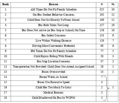
for write-ins was also provided. The complete list is given in Table 3.4 in descending rank order. Eight reasons were added to the original ten that best categorized “write-in” responses.
Table 3.4 Reasons Parents Choose Not To Use the School Bus Service
Rank Reason # %
1 AM Times Do Not Fit Family Schedule 325 20
2 On-Bus Student Behavior Concerns 192 12
3 Child Does Not Go Directly To/From School 189 12
4 Bus Ride Takes Too Long 157 10
5 Bus Does Not Arrive (at Bus Stop or School) On Time 156 10
6 Bus Safety Concerns 153 9
7 Live Within Walking Distance 120 7
8 Driving More Convenient/ Preferred 98 6
9 PM Times Do Not Fit Family Schedule 77 5
10 Child Enjoys Riding With Friends 58 3
11 Bus Stop Location Concerns 37 2
12 Transportation Not Provided/ Child Does Not Attend Assigned School 28 2
13 Buses Overcrowded 13 1
14 Parent Works At School 7
15 Buses Use Excessive Speed 3
16 Child Has Too Much To Carry 2 1
17 Medical Reasons 2
18 Child Disallowed On Bus by WCPSS 2
bell times are staggered and bus routes “tiered” in order to use individual buses for multiple routes. High school morning bell times occur mostly at 7:30 am or 8:00 am (WCPSS 2003). Middle and elementary school bell times range from 7:45 am to 9:15 am. This bell schedule requires that the first student on many high school bus routes be picked up between 6:00 and 6:30 am. This further decreases the chance of a significant modal shift to the school bus for high school students because scheduled morning arrival times are the primary reason that students do not ride. AVL technologies can increase the school bus level of service, but do not affect the scheduled arrival time of the school bus and therefore would not likely cause a modal shift amongst high school students.
Choice of driving as a mode of school transport and bell time schedules distinguish high school students from K-8 students, who have a different set of decision factors and travel characteristics. For this reason, the research focus was narrowed to grades K-8 in the school transportation mode choice model development process detailed in Chapter 4.
school bus, and non-motorized (pedestrian/bicycle) modes of school transportation. The remainder of Chapter 3 continues to consider the K-12 results of the preliminary survey.
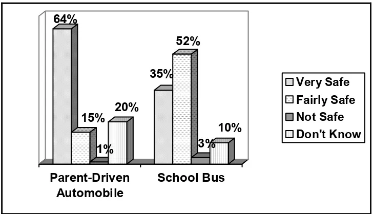
3.4.3 Perceived Modal Safety
sibling driving, are omitted because of small sample sizes; the majority of respondents did not rate these modes. Nearly 65% of parents rated driving their children to school as “very safe,” while only 35% of parents rated the school bus as “very safe.”
The benefits of a modal shift from the automobile to the school bus for school travel include decreasing the number of passenger cars on and around school campuses thereby decreasing conflict points and ultimately increasing safety. In order to prompt a modal shift, however, the parent-identified problems with the school bus service need to be addressed and improved.
64%
15%
1% 20%
35% 52%
3% 10%
Parent-Driven Automobile
School Bus
Very Safe Fairly Safe Not Safe Don't Know
Figure 3.2 Parental Safety Rating of Two Primary School Transportation Modes
3.4.4 Identified Problems with School Bus Service
WCPSS bus arrival times occurring around 6 am, students have to wait outside in the dark during winter months, adding to parental reluctance to use the school bus service. Student behavior on the bus and at bus stops is another major concern of parents, followed by concern about the bus adhering to the provided schedule. Parents do not want to leave for work and have their children at home or at a corner bus stop waiting for a school bus that may or may not arrive.
Some reasons that were given for not using the school bus service are unrelated to school bus system performance, like before and after school activities. Policy changes that require students to attend neighborhood schools may be the only viable solution to the long bus rides required to transport students across the county, but such changes are beyond the scope of this research. The primary problems with the school bus service that can be addressed by this research for school transportation operations are:
o Parental perception of passenger vehicle and school bus safety, o Morning loading times/ patterns,
o Student bus/ bus stop behavior, and
o Bus arrival punctuality at the school, home, or bus stop.
population had a problem with the arrival time of their child’s bus. Increasing customer satisfaction for this portion of the population could help promote a modal shift to the school bus.
3.4.5 AVL Assessment
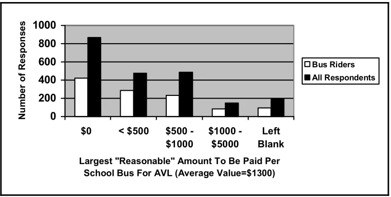
The final component of the preliminary survey was an assessment of parents’ acceptance of technologies aimed at solving problems with the school bus service. Parents were asked to indicate the price they deemed “reasonable” 1) to pay for in-home bus arrival notification/ paging technology and 2) for the school system to pay for bus tracking technology, regardless of whether their child rode the school bus. Approximately 48% of parents were unwilling to pay for an arrival notification service. Another 48% indicated a “willingness-to-pay” of $1 to $20 per month for this information. Based on the overall average, parents indicated that no more than approximately $7 per month would be “reasonable” to pay in order to subscribe to an AVL bus arrival notification service. In terms of AVL for school bus tracking, 40% of parents did not support the school system spending money on bus tracking technologies, but 51% did support spending in the range of $100 to $5000 per bus. The highest, “reasonable” amount to pay for tracking was found to be just over $1300 per bus based on the average responses. Figures 3.4 and 3.5 show the relationship of bus rider responses and total responses for the willingness-to-pay questions.
from Table 3.5 – gender, grade, and income – along with other factors, like travel distance and convenience, to develop the school transportation mode choice model.
18% 8%
1% 73%
On Time Early Late Unpredictable
Figure 3.3 Parental Assessment of School Bus Punctuality
0 200 400 600 800 1000 1200
$0 $1 - $4 $5 - $9 $10 -$14
$15 -$20
Left Blank Largest "Reasonable" Monthly Subscription Fee
(Average Value=$7) N u m b er of R espo n se s Bus Riders All Respondents
0 200 400 600 800 1000
$0 < $500 $500
-$1000
$1000 -$5000
Left Blank
Largest "Reasonable" Amount To Be Paid Per School Bus For AVL (Average Value=$1300)
Nu m b er of Respon se s Bus Riders All Respondents
Figure 3.5 Survey Responses on Willingness-to-Pay for AVL School Bus Tracking
Table 3.5 Profile of Student Characteristics by Mode
School Bus Passenger Vehicle Non-Motorized
Gender Male Female Male
Grade Level Middle High Elementary
District East Wake Sanderson Sanderson
3.5 Spatial Analysis
and median income values averaged to obtain average median household incomes for each high school attendance boundary. This value was thought to be an adequate surrogate variable for actual household income of the decision-making parent-student team.
During GIS analysis, review of the survey data showed irreparable inconsistencies in parent’s indicated high school attendance boundary. Some parents answered according to the high school attendance boundary in which they lived, as requested, but other parents answered according to the high school their children attended or would attend. So, if a child attended a school other than the school to which they were assigned, which is not uncommon in Wake County, the parent might not have indicated the correct attendance boundary.
student lived, surveys were mistakenly mailed according to the school to which each student was assigned.
In order to generate a quality data set for school transportation mode choice model development, resurveying was needed. The basis for the second survey was established in the conclusions and identified errors from the preliminary survey.
3.6 Survey Error
non-sampling variable errors may “stem from the respondent, the interviewing process, supervising, coding, editing, and data entry (Andersen 1979).”
Random sampling with stratification was used in the preliminary survey to minimize sampling biases. The survey was mailed to an equal number of parents in each Wake County high school attendance boundary. Non-response bias must be considered since only 25% of the surveys were returned. If sample statistics closely match population parameters, the effects of non-response bias on the data set can be deemed negligible. “Making no adjustment for nonresponse implicitly assumes that nonrespondents do not differ from respondents in any characteristic of interest. The degree to which they do differ is proportional to the amount of bias introduced by ignoring nonrespondents (Andersen 1979).”
respectively. This is to be expected, however, and is explained by the over-sampling that occurred in the high school population. In terms of school bus ridership (Table 3.6), the sample and population percentages were found to be significantly different.
Table 3.6 Survey Responses by School Bus Ridership Status Ridership Status Survey Sample WCPSS Population
School Bus Rider 49% 53%
Nonrider 51% 47%
Despite these statistical differences, no adjustments were made to the preliminary survey data because concerns of bias shifted to the new survey data, which would be used in model development. New survey data were analyzed in an attempt to evaluate the effects, if any, of nonresponse bias. Those results are given in Section 4.2.
3.7 Preliminary Survey Summary
Preliminary survey results favor the development of a school transportation mode
choice model because the general characteristics of students using the three prominent modes are different in terms of grade, gender, and socioeconomic status, based on the average median household income values calculated for the attendance boundaries.
high school grade level because student drivers and their passengers do not choose their mode of travel based on problems with the school bus service. Instead, student drivers and their passengers are assumed to be better classified as “captive” travelers because of the social implications and freedoms associated with driving. For this reason, only the travel patterns of non-high school students were evaluated in mode choice model development.
The available school transportation modes for students differ according to the
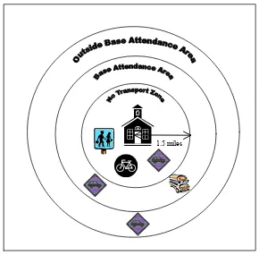
distance that a given student lives from his/her school. In North Carolina, state law mandates that a school district is not required to provide school bus transportation for students living within 1.5 miles of their school, unless potentially hazardous conditions exists, such as a child having to cross railroad tracks or multi-lane roads to get to school. Students living within the “no transport zone,” consisting of the 1.5-mile radius from a school, must therefore choose between the automobile and a non-motorized mode for school travel. Other students have a choice between school bus, automobile, or a non-motorized mode.
While a modal shift from passenger car to non-motorized modes for those living within walking distance of a school would be helpful in decreasing congestion around school campuses, the factors influencing decisions to walk or cycle to school, such as availability of sidewalks and trails, vary greatly by community. The task of creating a single model to estimate the mode split for more than one no-transport zone would be difficult because of the large variability in walking and biking conditions. The focus of further research was therefore set to non-high school students living outside of the no transport
4. MODEL DEVELOPMENT AND CALIBRATION
4.1 New Survey Structure
Resurveying was necessary to correct for bias of observation, caused by confusion amongst preliminary survey respondents regarding the high school attendance boundary in which they lived. The new survey also provided an opportunity to collect additional information not included in the preliminary survey, such as perceived home-to-school distance. In order to improve the survey process and the quality and usefulness of data collected, the following processes were changed in the new survey.
2. Wake County stratified by zip code- Confusion about high school attendance boundaries was alleviated by having respondents indicate their zip code. Also, because zip code boundaries are smaller than the high school attendance boundaries, parameters like household income that are averaged for each boundary were more accurate because they involved a smaller number of people. Representative coverage of the county was still achieved with zip code boundaries.
3. Focus shifted- Having established that high school students’ modal options differ significantly from elementary and middle school students, data were collected for students in grades K-8 only.
4. Sample size reduced- The methodology used to determine sample sizes for the original survey was discussed in detail in Section 3.2. Calculations supported sample sizes larger than 385 in order to achieve an expected error of less than 5%. Having experienced a 25% response rate and 1.8 student average per survey initially, the sample size for resurveying was set at 2000 in hopes of obtaining useful data on 500 to 1000 students.
believes that perceived distance would be more influential on mode choice than the actual distance because mode choice is based on the perception of the distance traveled. A problem may arise, however, in future school mode choice analyses that use the developed models since perceived distance data may not be readily available. Average perceived distances need to be computed by zip code for future applications of the model, if distance proves to be significant in forecasting mode choice.
4.2 New Survey Error
Nonresponse bias was again a primary concern, as with the preliminary survey, because of the 24% response rate for the new survey. In order to ensure that nonresponse did not have a measurable effect on the data, survey responses were analyzed in groups according to the average median household income for the associated zip code. A Wilcoxon two-sample test was completed for two income categories: income group one, consisting of the 16 Wake County zip code boundaries that have average median household incomes of $36,500 or less, and income group two, corresponding to the zip codes with incomes exceeding $36,500. Table 4.1 shows the data used for this analysis. For the responses in each zip code, the percent of the total sample was calculated, summing to 100% for the entire sample. The same was done for the number of students from the WCPSS population in each zip code. Ideally, the difference for each zip code between the percent of the sample and the percent of the population would be zero. The actual differences range from -3.7 percentage points to +5.4. The Wilcoxon two-sample test yielded statistics indicating a significant difference between the two income groups. The absolute value of the Z score test statistic for the percent differences would have to be less than 1.96, the Z score corresponding to a 95% confidence level, in order to accept the hypothesis that the two groups are identical. Similarly, the computed χ2 statistic would have to be less than the
critical χ2 value of 3.84, corresponding to a 95% level of confidence. The actual values of
Z and χ2 for the Wilcoxon two-sample test are 2.60 and 6.87, respectively. Both the
Z-score and χ2 exceed the critical values, meaning that the composite differences in the two
Table 4.1 New Survey Response Comparison with Overall Student Population
Zip Code
Income Group
# of Survey Responses
% of Sample
# in Student Population
% of Population
% Difference
27610 (Raleigh) 1 33 4.2 5035 7.9 -3.7
27604 (Raleigh) 1 16 2.0 3111 4.9 -2.8
27529 (Garner) 1 11 1.4 2686 4.2 -2.8
27526 (Fuquay Varina) 1 19 2.4 2654 4.2 -1.7
27603 (Raleigh) 1 20 2.6 2369 3.7 -1.1
27616 (Raleigh) 1 22 2.8 2528 4.0 -1.1
27607 (Raleigh) 1 8 1.0 1181 1.8 -0.8
27606 (Raleigh) 1 20 2.6 2155 3.4 -0.8
27591 (Wendell) 1 11 1.4 1332 2.1 -0.7
27597 (Zebulon) 1 1 0.1 491 0.8 -0.6
27601 (Raleigh) 1 8 1.0 838 1.3 -0.3
27545 (Knightdale) 1 29 3.7 2498 3.9 -0.2
27571 (Rolesville) 1 2 0.3 50 0.1 0.2
27605 (Raleigh) 1 3 0.4 87 0.1 0.2
27562 (New Hill) 1 4 0.5 128 0.2 0.3
27540 (Holly Springs) 1 33 4.2 2109 3.3 0.9
27511 (Cary) 2 31 4.0 5629 8.8 -4.8
27615 (Raleigh) 2 23 2.9 3169 5.0 -2.0
27609 (Raleigh) 2 15 1.9 2340 3.7 -1.7
27613 (Raleigh) 2 48 6.1 4181 6.5 -0.4
27592 (Willow Springs) 2 2 0.3 418 0.7 -0.4
27612 (Raleigh) 2 23 2.9 2009 3.1 -0.2
27617 (Raleigh) 2 8 1.0 644 1.0 0.0
27502 (Apex) 2 45 5.8 3222 5.0 0.7
27513 (Cary) 2 60 7.7 4061 6.4 1.3
27539 (Apex) 2 33 4.2 1376 2.2 2.1
27587 (Wake Forest) 2 33 4.2 1314 2.1 2.2
27523 (Apex) 2 32 4.1 843 1.3 2.8
27519 (Cary) 2 51 6.5 2328 3.6 2.9
27608 (Raleigh) 2 34 4.3 711 1.1 3.2
27614 (Raleigh) 2 46 5.9 1111 1.7 4.1
27560 (Morrisville) 2 58 7.4 1294 2.0 5.4
population. A t-test was used to verify the hypothesis that the sample and population percentages were equal against the two-sided alternative that they were different. No significant difference was found based on the computed t-statistics. The proportion of survey responses in each grade is therefore statistically equivalent to the proportion of the student population for that grade.
0 2 4 6 8 10 12 14
%
R
esp
o
n
ses
K 1 2 3 4 5 6 7 8
Grade
Sample Population
Figure 4.1 New Survey Responses by Student Grade Level
The survey sample yields AM and PM school bus mode shares of 53% and 66% respectively. WCPSS reports an average daily school bus ridership of 53% for the student population. There is a statistically significant difference between the PM reported bus ridership for the sample and the population. The computed t statistic exceeded 7.0 and the critical t value for 95% confidence is 1.96.
Yet, the data over-represent students from high-income families and school bus riders. This inconsistency suggests that the data quality may not be compromised by the difference in responses between high- and low-income groups.
The breakpoint used to differentiate high and low income groups is also a cause for the seeming nonresponse bias favoring high-income students. A value of $36,500 was selected as the breakpoint so that the high and low-income groups would have an equal number of zip codes boundaries for the Wilcoxon test. Selecting $36,500 as the breakpoint allowed the high- and low-income categories to each include 16 zip code boundaries. In Wake County, the median household income exceeds $50,000 so any breakpoint lower than this would likely prompt an overrepresentation of the higher income grouping.
In summary, the sample contains responses by grade that are similar to population percentages and does not underestimate school bus ridership as expected by a data set favoring high income families. For these reasons, no adjustments were made to the survey data prior to analysis for model development.
4.3 New Survey Analysis
attendance area for a school, beyond the no transport zone, is that boundary where school bus service is provided and the available modes are school bus and automobile. Nonmotorized modes are not feasible within the base attendance area, outside the no transport zone because of lengthy home-to-school distances. Finally, there are students living outside the base attendance area for the school they attend who are “automobile captive” because school bus service is not provided and distances make nonmotorized modes infeasible.
Figure 4.2 Student Transportation Zones
About 7% of students in the new survey live in a “no transport zone.” The actual number of students from this sample who live in a no transport zone may be much larger. Some parents may not be knowledgeable of the law concerning school bus transportation not being provided to students living within a 1.5 mile radius of their school (barring certain hazardous conditions) and would therefore not indicate that they live “within walking distance,” as defined by North Carolina state law. Another 1% of the students in the new survey sample use nonmotorized modes and were considered as living within the no transport zone, as were another 4% who use the automobile for school trips and listed perceived distances to school of 1.5 miles or less. So, the actual number of students in the no transport zone is expected to be between 7 and 12%.
School districts with “school choice” policies will likely have students outside the base attendance area. In Wake County, “students who are assigned outside their geographical area because of their request for a transfer (not magnet school) are not guaranteed transportation (WCPSS 2003).” About 1.5% of the students in the new survey are classified in this third group.
street connectivity, availability of bicycle infrastructure, building setbacks, and terrain (Rossi 2000). Components such as these are highly dependent upon the specific community or school being analyzed. The task of nonmotorized modeling for a model that will apply to an entire county or school district can be extremely difficult, so nonmotorized modes were not included in the model development analyses.
“Captive” travelers within the base attendance area were then identified. Captive is used to describe an involuntary state of being “because of a situation that makes free choice or departure difficult (Webster 1983).” The captive students within the base attendance area for the new survey are those who:
o must ride the school bus because their family does not own or have regular access to an automobile;
o must ride the school bus because parent work schedules prevent automobile pick-up; o have before and/ or after school activities that prevent riding the school bus; or
o are involved in before and/or after school care programs which provide van transportation to and from the school.