ABSTRACT
WILSON, DAVID HUNT. Signed Scale Measures: An Introduction and Application. (Under the direction of Dennis Boos and Jacqueline Hughes-Oliver.)
The role of the Interquartile Range in constructing a boxplot provides the rationale for considering the halves of the ”box” in a boxplot. The two halves of the boxplot are viewed as measures of distance from a measure of location. This viewpoint is the genesis for considering a new class of parameters called signed scale parameters.
A conceptual framework for signed scale parameters is introduced and four classes of signed scale parameters are discussed in detail. The small sample and asymptotic behaviors for several signed scale estimators are examined for nine distributions.
SIGNED SCALE MEASURES: AN INTRODUCTION AND APPLICATION
by
David Hunt Wilson
A thesis submitted to the Graduate Faculty of North Carolina State University
in partial fulfillment of the requirements for the Degree of
Doctor of Philosophy
DEPARTMENT OF STATISTICS
Raleigh 2002
APPROVED BY:
DENNIS BOOS JACQUELINE HUGHES-OLIVER
Co-chair of Advisory Committee Co-chair of Advisory Committee
Biography
Acknowledgement
Contents
LIST OF TABLES . . . vii
LIST OF FIGURES . . . ix
1 INTRODUCTION . . . 1
1.1 Signed Scale Measures and Estimators of Scale . . . 2
1.1.1 Scale Parameters and Estimation . . . 2
1.1.2 Signed Scale Parameters . . . 3
1.2 Classes of Scale and Signed Scale Parameters . . . 4
1.2.1 pthAbsolute Central Moment Class . . . 5
1.2.2 αthTrimmedpthAbsolute Central Moment Class . . . 5
1.2.3 Quantile Class . . . 6
1.2.4 A-estimator Class . . . 6
1.3 Classes of Signed Scale Estimators . . . 8
1.3.1 Signed Scale Estimators Derived FrompthAbsolute Central Moment Scale Parameters . . . 8
1.3.2 Signed Scale Estimators Derived FromαthTrimmedpthAbsolute Central Moment Scale Parameters . . . 9
1.3.3 Signed Scale Estimators Derived From Quantile Scale Parameters . . . 10
1.3.4 Signed Scale Estimators Derived From A-estimator Scale Parameters . . . 10
1.4 Properties of Signed Scale Estimators . . . 11
2 THEORY OF SIGNED SCALE ESTIMATORS . . . 14
2.1 Choosing Specific Signed Scale Estimators . . . 14
2.2.1 Consistency . . . 16
2.2.2 Asymptotic Normality . . . 23
2.2.3 Asymptotic Efficiency . . . 32
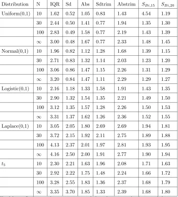
2.3 Small Sample Comparisons . . . 37
2.3.1 Symmetric Distributions . . . 38
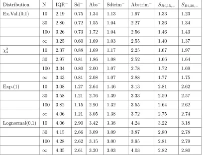
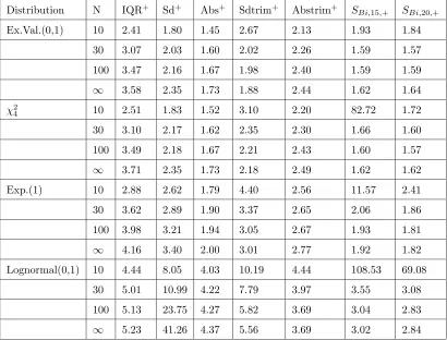
2.3.2 Skewed Distributions . . . 40
2.3.3 Summary of Simulation Results . . . 47
2.4 Recommendations . . . 47
3 A NEW RULE FOR GENERATING BOXPLOTS . . . 54
3.1 Motivation . . . 54
3.2 Signed Scale Boxplot Rule . . . 58
3.2.1 Example 1 . . . 62
3.2.2 Example 2 . . . 62
3.2.3 Example 3 . . . 65
3.3 Detecting Interesting Observations in Small Samples . . . 67
3.3.1 All-Inside Rate Per Sample . . . 67
3.3.2 Outside Rate Per Observation . . . 73
3.3.3 Outlier Detection . . . 78
3.3.4 Practical Consequences of the Signed Boxplot . . . 82
3.4 Skewness Information . . . 85
4 SUMMARY . . . 91
5 REFERENCES . . . 94
6 APPENDICES . . . 96
A.1 SPLUS Code For Signed Scale Estimators . . . 97
A.2 Deriving the Limiting Values of the Boxplot Fences . . . 100
List of Tables
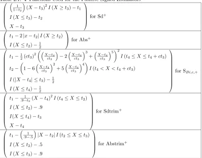
2.1 Ψ Functions Used for the Positive Signed Estimators . . . 25
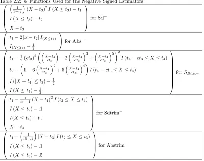
2.2 Ψ Functions Used for the Negative Signed Estimators . . . 26
2.3 Relationship Between Positive Signed Scale Estimators and Convenient Functionals . . . 26
2.4 Relationship Between Negative Signed Scale Estimators and Convenient Functionals . . . 27
2.5 Functionals Used To Derive Asymptotic Means of Positive Signed Estimators . . . 27
2.6 Functionals Used To Derive Asymptotic Means of Negative Signed Estimators . . . 27
2.7 Asymptotic Means for the Negative Signed Estimators Under Several Distributions . . . 31
2.8 Asymptotic Means for the Positive Signed Estimators Under Several Distributions . . . 32
2.9 Skewness and Kurtosis Ordering of Distributions . . . 32
2.10 Asymptotic Standardized Variances of the Negative Signed Estimators . . . 33
2.11 Asymptotic Standardized Variances of the Positive Signed Estimators . . . 34
2.12 Asymptotic Relative Efficiency of the Negative Signed Estimators . . . 35
2.13 Asymptotic Relative Efficiency of the Positive Signed Estimators . . . 35
2.14 Best and Second Best Performing Signed Estimators Along With Relative Efficiencies . . . 36
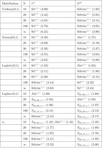
2.15 Small Sample Relative Efficiencies For Symmetric Distributions(+/−paired) . . . 39
2.16 Best Performing Estimators Under Symmetric Distributions(+/−paired) . . . 41
2.17 Finite Efficiencies For Negative Signed Estimators Under Skewed Distributions . . . . 43
2.19 Finite Efficiencies For Positive Signed Estimators Under Skewed Distributions . . . 45
2.20 Best Performing Positive Signed Estimators Under Skewed Distributions . . . 46
2.21 Standardized Variances For Positive and Negative Signed Estimators Under Symmetric Distributions. . . 48
2.22 Standardized Variances For Negative Signed Estimators Under Skewed Distributions. . . 49
2.23 Standardized Variances For Positive Signed Estimators Under Skewed Distributions. . . 50
2.24 Standardized Variances For Summed Estimators Under Symmetric Distributions. . . 51
2.25 Standardized Variances For Summed Estimators Under Skewed Distributions. . . 53
3.1 Limiting Values For the Common and Skew Adjusted Boxplots . . . 61
3.2 Limiting Values For the Signed Boxplot . . . 61
3.3 Annual Incomes of 69 Scientific and Literary Societies in England in 1840 . . . 62
3.4 Cranial Capacity of 17 Male Moriori Skulls . . . 62
3.5 15 Observations of the Vertical Semi-diameter of the Planet Venus . . . 65
3.6 Population Outside Rate Per Observation, as a Percentage . . . 74
3.7 Asymptotic and Estimated Means ofQC andQAbs . . . 90
List of Figures
3.1 Construction of a Hypothetical Boxplot . . . 55
3.2 Construction of a Skew Adjusted Boxplot . . . 56
3.3 Construction of a Signed Boxplot . . . 59
3.4 Incomes of the Top 69 Scientific and Literary Societies of England in 1840 . . . 63
3.5 Cranial Capacity of 17 Male Moriori Skulls . . . 64
3.6 Vertical Semi-Diameter Measurement Residuals of the Planet Venus . . . 66
3.7 All Inside Rate Per Sample Versus Sample Size for the Uniform Distribution . . . 69
3.8 All Inside Rate Per Sample Versus Sample Size for Symmetric Distributions . . . 70
3.9 All Inside Rate Per Sample Versus Sample Size for Skewed Distributions . . . 71
3.10 Outside Rate Per Observation Versus Sample Size for the Uniform Distribution . . . . 75
3.11 Outside Rate Per Observation Versus Sample Size for Symmetric Distributions . . . . 76
3.12 Outside Rate Per Observation Versus Sample Size for Skewed Distributions . . . 77
3.13 Outlier Detection Comparisons −N=10, Delta=0 . . . 79
3.14 Outlier Detection Comparisons −N=10, Delta=2 . . . 80
3.15 Outlier Detection Comparisons −N=10, Delta=3 . . . 80
3.16 Outlier Detection Comparisons −N=10, Delta=6 . . . 81
3.17 Outlier Detection Comparisons −N=30, Delta=0 . . . 81
3.18 Outlier Detection Comparisons −N=30, Delta=1 . . . 83
3.19 Outlier Detection Comparisons −N=100, Delta=0 . . . 83
Chapter 1
INTRODUCTION
The discipline of Statistics is often used to make comparisons and to examine data. An investigator may be interested in comparing the characteristics of different populations or comparing the behavior of one statistic relative to another. One particular method of investigation and comparison is known as the boxplot and was introduced by Tukey (1977). The boxplot is a graphical method of summarizing data and is used to quickly gain information about location, spread, and skewness.
Various modifications of Tukey’s boxplot have been introduced over the years, yet most of them rely on one particular notion of scale, the interquartile range (IQR), which is the difference between the third and first quartiles. While the IQR is relatively easy to calculate, especially for small sample sizes, it is most often a less efficient measure of scale than other scale estimators such as the standard deviation and mean absolute deviation. However, one way in which the boxplot provides information about skewness is via the distance of the median from the first quartile and the distance of the median from the third quartile. If the median is closer to the first quartile then the data (or distribution) is said to be skewed to the right. Conversely, if the median is closer to the third quartile then the distribution is said to be skewed to the left.
parameters when describing a population) since IQR+ only uses values greater (+) than a measure of location and IQR−only uses values less than (−) that measure of location. This dissertation will introduce the notion of signed scale measures and provide an example illustrating a use for signed scale measures in the area of exploratory data analysis.
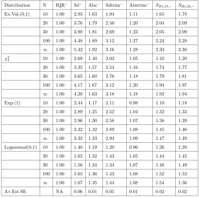
The remainder of this chapter will define signed scale parameters and list properties they should satisfy. The notion of signed scale estimators follows and several classes of signed scale estima-tors are introduced. Chapter 2 will examine the asymptotic and small sample properties of several signed scale estimators under the Uniform(0,1), Normal(0,1), Laplace(0,1),t5, Logistic(0,1), Expo-nential(1), χ24, Extreme Value(0,1), and Lognormal(0,1) distributions. Lastly, Chapter 3 uses the notion of signed scale estimators to introduce a new type of boxplot. The new boxplot will be compared and contrasted with two other boxplot types with respect to its ability to detect unusual observations and provide information about skewness, both for small samples and asymptotically.
1.1
Signed Scale Measures and Estimators of Scale
1.1.1
Scale Parameters and Estimation
LetXbe a random variable with distribution functionFX, and letS(F) be a functional defined for
distribution functionsF. Following the work of Ferguson (1967, p.164),S(FX) is a scale parameter
for the distribution of the random variableX if it satisfies the following properties: 1. Positivity: S(FX)≥0.
2. Translation Invariance: S(FX) is also a scale parameter for the distribution of the random variablea+X, where ais a finite constant.
3. Equivariance: |b|S(FX) is a scale parameter for the distribution of the random variablebX,
where bis a finite constant.
A common problem in statistics is the estimation of scale parameters through various techniques, such as maximum likelihood and the method of moments. The estimators derived through these techniques should satisfy properties similar to those of the parameters being estimated. Specifically, letxn = (x1, . . . , xn)T be a random sample from a distribution FX with scale parameter S(FX),
and let the sample distribution function be denoted Fxn. A statistic S(Fxn) will be viewed as a scale estimator if it satisfies three properties:
2. Translation Invariance: S(Fa+xn) =S(Fxn), whereais a finite constant, andFa+xn denotes the sample distribution function for the sample with ithelementa+x
i.
3. Equivariance: S(Fbxn) =|b|S(Fxn), wherebis a finite constant, andFbxn denotes the sample distribution function for the sample withithelement bx
i.
The scale estimators considered in this paper satisfy these properties. In general, any estimator mentioned that satisfies these properties will be referred to as a scale estimator.
While the definition of scale parameter is convenient, and many estimation techniques exist that yield estimators with desirable properties, there is no guarantee that distributions from different classes will have scale parameters that have the same interpretation or are directly comparable. Moreover, scale estimators that have desirable properties under one distribution may have undesir-able properties under another.
1.1.2
Signed Scale Parameters
The concept of signed scale parameters is an extension of the concept of scale parameters. However, each scale parameter is associated with two signed scale parameters, a “positive” and a “negative” parameter. The terms “positive” and “negative” do not denote the sign of the scale parameter, but rather whether the scale estimator uses values larger than some location measure or smaller than some location measure in its construction. Conceptually, a positive signed scale parameter reflects the variability of a distribution above some specified location measure and a negative signed scale parameter reflects the variability below the specified location measure. Typically, the specified location measure is a measure of central tendency, such as the mean or median.
To define our signed scale functionals it is simplest to use scale functionals S(F) for positive random variablesY (see Bickel and Lehmann 1976, p. 1152, although we do not require stochastic ordering). We define such functionals to satisfy
1. Positivity: S(FY)≥0.
2. Equivariance: S(FbY) =bS(FY) forb >0.
Discussion of signed scale parameters will be restricted to continuous random variables with positive density at a central measure of locationµ(F). LetXbe a random variable with distribution function F and with a measure of location µ(F). It is assumed thatµ(F) satisfies µ(Fa+bX) = a+bµ(FX) for constants aandb. Apositive signed scale functional T+ measures scale or average distance aboveµ(F) and satisfies
2. Translation invariance: T+(Fa+X) =T+(FX) for finite constant a. 3. Equivariance: T+(FbX) =bT+(FX) for constantb >0.
Negative signed scale functionals T− measure scale below µ(F) and satisfy the above three properties withT− replacingT+ above.
Generally we define our signed scale functionals via scale functionals for positive random variables as follows. Suppose that S is a scale functional for a positive random variable as defined above. Following the work of Bickel and Lehmann (1976), ifS(F) is a scale parameter for the distribution of a positive random variableX, then a positive signed scale parameter is a functionalT+(F) defined by the relationship
T+(F) =S(F+) (1.1)
where
F+(x) = F(x+µ(F))−F(µ(F))
1−F(µ(F)) forx >0 (1.2)
is just the distribution function of |X−µ(F)| conditional on X > µ(F). Similarly, a negative signed scale parameter is a functionalT−(F) defined by the relationship
T−(F) =S(F−) (1.3)
where
F−(x) =F(µ(F))−F(µ(F)−x)
F(µ(F)) forx >0 (1.4)
is just the distribution function of|X−µ(F)|conditional onX < µ(F).
It is easy to verify that T+(F) and T−(F) as defined above from scale functionals for positive random variables satisfy the definition of signed scale functionals.
1.2
Classes of Scale and Signed Scale Parameters
Scale parameters, and thus signed scale parameters, can be classified into various classes. Four such classes of scale parameters are the pth absolute central moment class, the αth trimmed pth
1.2.1
p
thAbsolute Central Moment Class
Given a random variableX with distribution functionF and measure of locationµ(F), thepth
absolute “central” moment ofF is defined as
Tp(F) = [EF|X−µ(F)|p]1/p=
+∞
−∞ |x−µ(F)|
pdF(x)
1/p .
This is a slight abuse of terminology since this phrase is usually used only when the center or measure of location is the mean. The quantityTp(F) is often used as a measure of the scale of a distribution. Common values of p are 1 and 2, and µ(F) is typically the mean or median. The related scale functional for a positive random variableX is
Sp(F) =
+∞
0 |x|
pdF(x)
1/p .
Following the definition of a positive signed scale parameter as given by (1.1) and (1.2), the positivepthabsolute central moment scale parameter is
Tp,+(F) =
1 1−F(µ(F))
∞
µ(F)|
x−µ(F)|pdF(x)
1/p ,
while the negativepthabsolute central moment scale parameter is obtained from (1.3) and (1.4) as
Tp,−(F) =
1
F(µ(F))
µ(F)
−∞ |x−µ(F)|
p dF(x)
1/p .
1.2.2
α
thTrimmed
p
thAbsolute Central Moment Class
Given a random variable X with distribution function F and measure of locationµ(F), and a numberα∈(0, .5), then the αthtrimmedpthabsolute central moment ofF is defined as
Tp,α(F) =
F−1(1−α)
F−1(α) |
x−µ(F)|pdF(x)
1/p .
The quantity Tp,α(F) is said to be a trimmed measure of scale. Common values of p are 1 and 2, while common values of αare 0.05 and 0.1. The related scale functional for a positive random variableX is
Sp,α(F) =
F−1(1−α)
0 |x|
p dF(x)
1/p .
signedαth trimmedpthabsolute moment scale parameter is
Tp,α,+(F) =
1
1−α−F(µ(F))
F−1(1−α)
µ(F) |
x−µ(F)|pdF(x)
1/p ,
while the negative αth trimmed pth absolute moment scale parameter is obtained from (1.3) and (1.4) as
Tp,α,−(F) =
1
F(µ(F))−α
µ(F)
F−1(α)
|x−µ(F)|pdF(x)
1/p .
1.2.3
Quantile Class
Let X be a random variable with distribution function F and let α∈ (0, .5), then a quantile measure of scale is written as
Tα(F) =F−1(1−α)−F−1(α).
The related scale functional for a positive random variableX is
Sα(F) =F−1(1−α).
One of the simplest notions of scale, the IQR, can be expressed simply asT0.25(F). Notice that
Tα(F) can be expanded and written as
Tα(F) =F−1(1−α)−F−1(.5) +F−1(.5)−F−1(α) .
Now letting the central measure of location beF−1(.5), the corresponding positive signed quantile scale measure as obtained from (1.1) and (1.2) is
Tα,+(F) =F−1(1−α)−F−1(.5),
and the corresponding negative signed quantile scale measure given by (1.3) and (1.4) is
Tα,−(F) =F−1(.5)−F−1(α).
1.2.4
A-estimator Class
with sample distribution functionFxn from a Normal(0,σ2) distribution. Then,n·var(x) =σ2. In such a situation, the square root ofntimes the sample standard deviation of the location estimator
xcan be used as a estimator of scale.
Following the work of Lax (1985), an A-estimate of scale is defined analogously from the asymp-totic variance of a location estimator. Specifically, given a scale estimateS(Fxn), distribution F, a positive constantc, and a function Ψ, the M-estimate of location is defined to be the solutionµ(Fxn) of the following equation due to Huber (1964): ni=1Ψ ((xi−µ(Fxn))/cS(Fxn)) = 0. Under certain
regularity conditions and whenF is a symmetric distribution,
µ(Fxn) is AN(µ(F), AΨ,F/n)
where
AΨ,F = (cS(F))2
∞
−∞Ψ2(u)dF(x)
∞
−∞Ψ(u)dF(x)
2
is the asymptotic variance of the M-estimator of location based on the function Ψ and with data coming from distributionF whereu= (x−µ(F))/cS(F).
Now, the function Ψ can be used to limit the influence of points far from the estimated center
µ(Fxn) of the sample. Huber, for example, proposed the function
ΨH(u) =
−b u <−b u −b≤u≤b
b u > b
for some b > 0. This function gives less weight to those observations whose values are larger in magnitude thanb. In terms of A-estimators, if observations are far away from the center, then they receive less weight than observations close to the center.
So, for a random variableXwith distribution functionF, a constantc, a scale parameterS(F), a location parameterµ(F), and a function Ψ, an A-estimator scale parameter is defined to be (AΨ,F)12 and can be written as
TΨ,c(F) = (AΨ,F)
1 2 =
(cS(F))
2
∞
−∞Ψ2(u)dF(x)
∞
−∞Ψ(u)dF(x)
2
1/2
The related scale functional for a positive random variableX is
SΨ,c(F) =
(cS(F))2
∞
0 Ψ2(u)dF(x)
∞
0 Ψ(u)dF(x)
2
1/2
whereu=x/cS(F).
Applying the definition of positive signed scale parameter as given by (1.1) and (1.2), the positive signed A-estimator scale parameter is
TΨ,c,+(F) =
(cS(F))
2(1−F(µ(F)))
∞
µ(F)Ψ2(u)dF(x)
∞
µ(F)Ψ(u)dF(x)
2
1/2 .
Notice that this signed parameter deviates slightly from the strict definition of a positive signed scale parameter because the scale parameterS(F) is based on observations belowµ(F).
Similarly, the negative signed A-estimator scale parameter follows from (1.3 and (1.4) as
TΨ,c,−(F) =
(cS(F))
2F(µ(F))
µ(F)
−∞ Ψ2(u)dF(x)
µ(F)
−∞ Ψ(u)dF(x)
2
1/2
.
Again, this parameter does not strictly follow the definition of a negative signed scale parameter due to the inclusion ofS(F).
1.3
Classes of Signed Scale Estimators
The formulation of the four classes of signed scale parameters in terms of functionals readily allows creation of corresponding classes of estimators by evaluating the functionals under the sample distributionFxn. The forms of the estimators for the four classes of signed scale parameters are as follows.
1.3.1
Signed Scale Estimators Derived From
p
thAbsolute Central
Mo-ment Scale Parameters
Given a sample xn = (x1, . . . , xn) with sample distribution function Fxn, an estimator of the positive signed scale parameterTp,+(F) is
Tp,+(Fxn) =
1
1−Fxn(µ(Fxn)) 1
n
|xi−µ(Fxn)|pI(xi ≥µ(Fxn))
which can be simplified to
Tp,+(Fxn) =
1
I(xi≥µ(Fxn))
|xi−µ(Fxn)|pI(xi≥µ(Fxn))
1/p .
Similarly, an estimator of the negative signed scale parameterT−,p(F) is
Tp,−(Fxn) =
1
Fxn(µ(Fxn))
1
n
|xi−µ(Fxn)|pI(xi≤µ(Fxn))
1/p
which also can be simplified to
Tp,−(Fxn) =
1
I(xi≤µ(Fxn))
|xi−µ(Fxn)|pI(xi ≤µ(Fxn))
1/p .
1.3.2
Signed Scale Estimators Derived From
α
thTrimmed
p
thAbsolute
Central Moment Scale Parameters
Given a sample xn = (x1, . . . , xn) with sample distribution function Fxn, an estimator of the
positive signed trimmed scale parameterTp,α,+(F) is
Tp,α,+(Fxn) =
1
1−α−Fxn(µ(Fxn)) 1
n
|xi−µ(Fxn)|pI
µ(Fxn)≤xi ≤Fx−n1(1−α)
1/p
which can be reduced to
1
Iµ(Fxn)≤xi ≤Fx−n1(1−α)
|xi−µ(Fxn)|pIµ(Fxn)≤xi≤Fx−n1(1−α)
1/p .
An estimator of the negative signed trimmed scale parameter T−,p,α(F) is
Tp,α,−(Fxn) =
1
Fxn(µ(Fxn))−α
1
n
|xi−µ(Fxn)|pIFx−n1(α)≤xi≤µ(Fxn) 1/p
which is reducible to
1
IFx−n1(α)≤xi≤µ(Fxn)
|xi−µ(Fxn)| p
IFx−n1(α)≤xi≤µ(Fxn)
1.3.3
Signed Scale Estimators Derived From Quantile Scale
Parameters
Given a sample xn = (x1, . . . , xn) with sample distribution function Fxn, an estimator of the positive signed quantile scale measureTα,+(F) is just
Tα,+(Fxn) =Fx−n1(1−α)−Fx−n1(.5),
and, similarly, an estimator of the negative signed quantile scale measureT−,α(F) is just
Tα,−(Fxn) =Fx−n1(.5)−Fx−n1(α).
1.3.4
Signed Scale Estimators Derived From A-estimator Scale
Parameters
Since A-estimator class scale parameters depend on a location parameter and a scale parameter, following the work of Lax (1985), all A-estimator class scale parameters considered will use the median as the location parameter and the median absolute deviation from the median (MAD) as the scale parameter. With these guidelines in mind, given a samplexn = (x1, . . . , xn) with sample
distribution functionFxn, an estimator of the positive signed A-estimator scale parameterTΨ,c,+(F) is
TΨ,c,+(Fxn) =
(cS(Fxn))21−FxnFx−n1(.5) 1
n
Ψ2(ui)I(ui>0)
1
n
Ψ(ui)I(ui>0)2
1/2
whereui=xi−Fx−n1(.5) /cS(Fxn). This can be simplified to
TΨ,c,+(Fxn) =
n
2(cS(Fxn))
2 Ψ2(ui)I(ui>0)
[Ψ(ui)I(ui>0)]2
1/2
.
In Monte Carlo studies performed by Lax (1985), the Ψ function that yielded the best relative efficiency of A-estimators of scale was the bisquare function. The bisquare function is defined as
Ψ (ui) =ui
1−u2i 2I(−1<ui<1)
whereui = (xi−t)/cSfor some chosentandS. Notice that this function is different from Huber’s
A function Ψ (u) is redescending if Ψ (u)→0 asu→ ∞. Accordingly, the bisquare function gives observations far away from the center little or no weight, while non-decreasing functions, such as Huber’s, always give some weight to outlying observations. All further A-estimator class scale parameters and the derived estimates will use only the bisquare function. Using this function, the form of the estimator of the positive signed A-estimator scale parameter reduces to
TΨ,c,+(Fxn) =
n
2 (cS(Fxn))
2 u2i
1−u2i 4I(0< ui<1)
[(1−u2i) (1−5u2i)I(0< ui<1)]2
1/2 .
Following similar logic, an estimator of the negative signed A-estimator scale parameter is
TΨ,c,−(Fxn) =
n
2(cS(Fxn))
2 u2i
1−u2i 4I(−1< ui<0) [(1−u2i) (1−5u2i)I(−1< ui<0)]2
1/2
whereui=
xi−Fx−n1(.5) /cS(Fxn).
1.4
Properties of Signed Scale Estimators
Since signed scale estimators derive from regular scale estimators, it is reasonable to require that any potential signed scale estimator have properties similar to unsigned scale estimators. While there are other properties of scale estimators that could be specified (Bickel and Lehmann 1976), given a samplexn= (x1, . . . , xn) and sample distribution function denotedFxn, it will be required
that signed scale estimatorsT+(Fxn) andT−(Fxn) satisfy the following three properties 1) Positivity T+(Fxn)≥0,T−(Fxn)≥0 for anyxn.
2) Translation Invariance T+(Fa+xn) =T+(Fxn),T−(Fa+xn) =T−(Fxn) for finite constanta.
3) Equivariance T+(Fbxn) =bT+(Fxn),T−(Fbxn) =bT−(Fxn) for constantb >0.
Lemma 1 Signed scale estimators satisfy the three properties.
Proof. Letxn = (x1, . . . , xn) be a random sample from distribution function FX with sample distribution functionFxn. SinceT+(Fxn) =S(Fxn,+) and sinceSis assumed to be a scale estimator, then all positive signed scale estimators satisfy the three properties. Additionally, sinceT−(Fxn) =
S(Fxn,−) then all negative signed scale estimators satisfy the three properties.
Lemma 2 A-estimator class derived signed scale estimators satisfy the three properties.
functionFxn, letaandb >0 be arbitrary constants, andui=xi−Fx−n1(.5) /cS(Fxn). Then,
TΨ,c,+(Fxn) =
n
2(cS(Fxn))
2 u2i
1−u2i 4I(0< ui<1) [(1−u2i) (1−5u2i)I(0< ui<1)]2
1/2
satisfies property 1 because the numerator is the sum of positive quantities and the denominator is squared. Now consider the perturbed sample with ith component a+bx
i, and denote the sample
distribution function of this new sample byFa+bxn. Then,
TΨ,c,+Fa+bxn =
n
2
cS
F a+bxn
2 µ2i1−µ2i 4I(0< µi<1)
[(1−µ2i) (1−5µ2i)I(0< µi <1)]2
1/2
where µi=
(a+bxi)−Fa−+1bxn(.5)
/cSFa+bxn . BecauseFa−+1bx
n(.5) =a+bF
−1
xn (.5), µi can be
written asbxi−Fx−n1(.5) /cSFa+bxn . Lettingmedian(xi) =median(xn),
S(Fxn) =median(|xi−median(xn)|, i= 1, ..., n) and
SFa+bxn =median(|(a+bxi)−median(a+bxn)|, i= 1, ..., n)
which can be simplified to
SFa+bxn =|b|median(|xi−median(xn)|, i= 1, ..., n).
Because we assumeb >0, this reduces to
SFa+bxn = (b)median(|xi−median(xn)|, i= 1, ..., n) =bS(Fxn).
Therefore,µi can be written as
µi=bxi−Fx−n1(.5) /cSFa+bxn =bxi−Fx−n1(.5) /cbS(Fxn) =xi−Fx−n1(.5) /cS(Fxn).
ThusTΨ,c,+Fa+bxn can be written as
n
2(cbS(Fxn))
2 u2i
1−u2i 4I(0< ui<1)
[(1−u2i) (1−5u2i)I(0< ui<1)]2
which equals
b
n
2 (cS(Fxn))
2 u2i
1−u2i 4I(0< ui <1)
[(1−u2i) (1−5u2i)I(0< ui<1)]2
1/2
=bTΨ,c,+(Fxn),
showing that properties 2 and 3 hold. By similar arguments, properties 1 through 3 hold for
Chapter 2
THEORY OF SIGNED SCALE
ESTIMATORS
2.1
Choosing Specific Signed Scale Estimators
A subset of the four classes of signed scale estimators was selected for further comparison. From thepthAbsolute Moment Class of estimators was chosen the pair of signed estimators Sd+and Sd−,
wherep= 2 andµ(Fxn) =x, defined as
Sd+=
1
I(xi≥x)
|xi−x|2I(xi≥x)
1/2
and
Sd−=
1
I(xi≤x)
|xi−x|2I(xi≤x)
1/2 .
From the same class, the pair of signed estimators Abs+ and Abs− , wherep= 1 and u(Fxn) =
Fx−n1(.5), were also selected. These estimators are defined as
Abs+= 1
Ixi ≥Fx−n1(.5)
xi−Fx−n1(.5)Ixi≥Fx−n1(.5)
and
Abs− = 1
Ixi≤Fx−n1(.5)
The pair of signed estimators Sdtrim+ and Sdtrim−, with α= .1, p = 2, and u(Fxn) = xwere chosen from theαth TrimmedpthAbsolute Moment Class and are defined as
Sdtrim+=
1
Ix≤xi≤Fx−n1(.9)
|xi−x|2Ix≤xi≤Fx−n1(.9)
1/2
and
Sdtrim−=
1
IFx−n1(.1)≤xi≤x
|xi−x|2IFx−n1(.1)≤xi≤x
1/2 .
Another pair of signed estimators, Abstrim+ and Abstrim−, withα=.1,p= 1, and
u(Fxn) =Fx−n1(.5), were picked from the same classes and are defined as
Abstrim+= 1
IFx−n1(.5)≤xi ≤Fx−n1(.9) xi−F
−1 xn (.5)I
Fx−n1(.5)≤xi≤Fx−n1(.9)
and
Abstrim−= 1
IFx−n1(.1)≤xi≤Fx−n1(.5)
xi−Fx−n1(.5)IFx−n1(.1)≤xi ≤Fx−n1(.5) .
From the Quantile class of estimators comes IQR+ and IQR− which are defined as
IQR+=Fx−n1(.75)−Fx−n1(.5)
and
IQR− =Fx−n1(.5)−Fx−n1(.25).
The last set of estimators are derived from the A-estimator class. Since the Ψ function, center of location T, and measure of scale S are picked to be the bisquare function, median, and median absolute deviation from the median, then the entire set of estimators derived from this class differs only in the choice of the constant c. Positive and negative signed estimators derived from this class are denoted bySBi,c,+ andSBi,c,−, respectively, whereBiindicates the choice of the bisquare function for Ψ. SBi,c,+ andSBi,c,− estimators are considered forc= 15 and c= 20. The form of
these estimators is
SBi,c,+=
n
2(cS(Fxn))
2 u2i
1−u2i 4I(0< ui<1)
[(1−u2i) (1−5u2i)I(0< ui <1)]2
and
SBi,c,− =
n
2 (cS(Fxn))
2 u2i
1−u2i 4I(−1< ui<0)
[(1−u2i) (1−5u2i)I(−1< ui<0)]2
1/2
where S(Fxn) is the median of xi−Fx−n1(.5) and ui =xi−Fx−n1(.5) /cS(Fxn). The following sections examine the asymptotic and small sample properties of these seven pairs of estimators.
2.2
Asymptotic Properties
2.2.1
Consistency
The signed scale estimators considered are weakly consistent under certain conditions. The following theorem by Stefanski (1997, personal communication) will be helpful in establishing the consistency of Abs+, Abs−, Sd+, and Sd−.
Theorem 1 Let X1, . . . ,Xn be i.i.d. random vectors from a distributionFX, θ0 a finite constant,
g(x, θ)a real-valued function, andθn an estimate ofθ0. Then under the following conditions 1) There exists a neighborhood N(θ0)of θ0 such that g(x, θ) is a monotone function ofθ forθ ∈ N(θ0)and for allxin the support of X1.
2)H(θ) =E{g(X1, θ)} exists and is finite in a neighborhood ofθ0 and is continuous atθ0.
1
n n
i=1 g
Xi,θn
p
−→H(θ0) as n−→ ∞ as long asθn−→p θ0 as n−→ ∞.
Proof. Assume without loss of generality that g is nondecreasing. Lettn = n1ni=1g
Xi,θn
andtn =n1in=1g(Xi, θ0). Then, forδ >0,
tn−tn=tn−tnIθn−θ0> δ
+tn−tnIθn−θ0≤δ
=Rn,1+Rn,2.
For anyε >0
P(Rn,1> ε)≤Pθn−θ0> δ
Now, givenε >0, chooseδε>0 such that|H(θ0+δε)−H(θ0−δε)|< ε2, then
Rn,2=
1 n n i=1 g
Xi,θn
− 1 n n i=1
g(Xi, θ0)
Iθn−θ0≤δε
≤ 1 n n i=1 g
Xi,θn
−g(Xi, θ0)Iθn−θ0≤δε
≤ 1 n n i=1
|g(Xi, θ0+δε)−g(Xi, θ0−δε)|Iθn−θ0≤δε
≤ 1 n n i=1
[g(Xi, θ+δε)−g(Xi, θ−δε)]
Call the last expressionWn and note that it is non-negative. Then, by the Markov inequality,
P(Rn,2> ε)≤P(Wn > ε)≤
E(Wn) ε <
ε2 ε =ε.
Therefore, Rn,1 and Rn,2 each converge in probability to zero. Noting that tn can be written
as tn+
tn−tn , and that tn −→p H(θ0) by the W.L.L.N., then n1
n i=1g
Xi,θ
p
−→ H(θ0) as
n−→ ∞.
The following Theorems 2 and 3 show consistency of signed scale estimators from thepthAbsolute Moment Class of estimators. Theorem 2 deals with positive signed estimators and Theorem 3 deals with negative signed estimators.
Theorem 2 LetX1, . . . , Xn be distributedi.i.d. F such thatE(|X1|I(X1>0))p<∞,µ(F)<∞, andF is continuous atµ(F). If µ(Fxn)→P µ(F), then
Tp,+(Fxn) =
1
1−Fxn(µ(Fxn)) 1
n
|xi−µ(Fxn)| p
I(xi≥µ(Fxn))
1/p P
→
1 1−F(µ(F))
∞
µ(F)
|X1−µ(F)|pdF
1/p
=Tp,+(F).
Proof. The denominator of the first ratio can be written as n1ni=1I(xi> µ(Fxn)). Letting g(x, θ) =I(x > θ), note thatg(x, θ) is a monotone decreasing function ofθ for fixedx.Also,
By assumption,H(θ) = 1−F(θ) is continuous atθ=µ(F). Thus the conditions of Theorem 1 hold and 1−Fxn(µ(Fxn))→P 1−F(µ(F)). And since the reciprocal function is continuous,
1
1−Fxn(µ(Fxn))
P
→ 1
1−F(µ(F)).
Lettingg(x, θ) =|x−θ|pI(x > θ), note thatg(x, θ) is monotone decreasing as a function ofθ for fixed x. Also note thatg(x, θ), when viewed as a function of θ for fixedx, is continuous for allθ. Now,
E|g(X1, θ)|=E(|X1−θ|pI(X1> θ))<∞ ∀θ sinceE(|X1|I(X1>0))p<∞
andE(g(X1, θ)) is continuous atθ=µ(F) since g(x, θ) is continuous inθ. Therefore, by Theorem 1,
1
n
|xi−µ(Fxn)|pI(xi≥µ(Fxn)) P
→
∞
µ(F)
|x−µ(F)|pdF(x).
Using these two convergence results, Slutsky’s theorem, and the fact that thepth root function is
continuous, then
Tp,+(Fxn) P
→Tp,+(F).
Corollary 1 Abs+ and Sd+ are positive signed estimators from the pth Absolute Moment Class of estimators where µ(Fxn) =Fx−n1(.5), p= 1 and µ(Fxn) =x, p= 2 , respectively. By Theorem 2,
these estimators converge in probability if Theorem 4 holds with p= 1/2 andE|X1|<∞.
Theorem 3 LetX1, . . . , Xn be distributedi.i.d. F such thatE(|X1|I(X1<0))p<∞andµ(F)< ∞. Ifµ(Fxn)→P µ(F), then
Tp,−(Fxn) =
1
Fxn(µ(Fxn)) 1
n
|xi−µ(Fxn)|pI(xi≤µ(Fxn))
1/p P
→
1
F(µ(F))
µ(F)
−∞ |x−µ(F)|
p dF(x)
1/p
=Tp,−(F).
Proof. Similar to Theorem 2.
Corollary 2 Abs− and Sd− are negative signed estimators from thepthAbsolute Moment Class of
The following theorem provided by Serfling (1980) will be useful in showing the consistency of estimators from the Quantile class.
Theorem 4 Let 0< p <1. If F−1(p) = inf{x:F(x)≥p} is the unique solution xof
F(x−)≤p≤F(x), thenFx−n1(p)wp→1F−1(p).
Theorem 4, along with Slutsky’s theorem, yields the following two theorems and corresponding corollaries.
Theorem 5 If F satisfies Theorem 4 forp= 1/2 andp= 1−α, thenTα,+(Fxn) =Fx−n1(1−α)− Fx−n1(.5) converges with probability 1 toTα,+(F) =F−1(1−α)−F−1(.5).
Corollary 3 Assuming the conditions of Theorem 5 forα=.25, IQR+=T.25,+(Fxn) =Fx−n1(.75)− Fx−n1(.5) converges with probability 1 toT.25,+(F) =F−1(.75)−F−1(.5).
Theorem 6 IfF satisfies Theorem 4 forp= 1/2andp=α, thenTα,−(Fxn) =Fx−n1(.5)−Fx−n1(α)
converges with probability 1 toTα,−(F) =F−1(.5)−F−1(α).
Corollary 4 Assuming the conditions of Theorem 6 forα=.25, IQR−=T.25,−(Fxn) =Fx−n1(.5)− Fx−n1(.25)converges with probability 1 toT.25,−(F) =F−1(.5)−F−1(.25).
Consistency of estimators derived from theαthTrimmedpthAbsolute Moment and the
A-estimator classes follows by relying upon the notion of U-statistics with estimated parameters (Iverson and Randles 1989). For statistics of the formUn
λn
= 1nni=1h
Xi,λn
whereλn is an
estimator of a population parameterλ, consistency will follow from Theorem 7 due to Iverson and Randles (1989).
Theorem 7 Suppose thatE|h(X1;λ)|<∞and that there is a neighborhood K(λ)ofλ, such that if D(λ, d)is a sphere centered at λwith radiusdsatisfying D(λ, d)⊂K(λ), then
(i) lim
d→0 E
sup
γ∈D(λ,d)|h(X1;γ)−h(X1;λ)|
= 0. Under these assumptions:
(A)If λn−→P λ, thenUn
λn
P
−→Eλh(X1;λ).
(B)If λn W P−→1λ, thenUn
λn
W P−→1
Eλh(X1;λ).
For positive signed estimators derived from theαthTrimmedpthAbsolute Moment Class,
Theorem 8 Let X1, . . . , Xn be distributedi.i.d. F such that E|X1|p<∞forp≥1 and
µ(F)<∞. Then
1
1−α−Fxn(µ(Fxn)) 1
n
|xi−µ(Fxn)| p
Iµ(Fxn)≤xi≤Fx−n1(1−α)
1/p P
→
1
1−α−F(µ(F))
F−1(1−α)
µ(F)
|x−µ(F)|pdF(x)
1/p
if µ(Fxn)converges in probability toµ(F). Ifµ(Fxn)converges wp1 toµ(F), then the above
convergence is wp1.
Proof. The quantity n1|xi−µ(Fxn)|pIµ(Fxn)≤xi≤Fx−n1(1−α) can be viewed as a U-Statistic with estimated parametersFx−n1(1−α) andµ(Fxn), kernel
h(X1, γ= (γ1, γ2)) =|X1−γ1|pI(γ1≤X1≤γ2) ,
andθ(γ) =Eλ[h(X1;γ)] whereλ=µ(F), F−1(1−α) . First,
E[|h(X1, γ)|] =E[|X1−γ1|pI(γ1≤X1≤γ2)]≤E[|X1−γ1|p]<∞
sinceE|X1|p<∞. Second,
|h(X1, γ)−h(X1, λ)|=||X1−γ1|pI(γ1≤X1≤γ2)− |X1−λ1|pI(λ1≤X1≤λ2)|
≤ ||X1−λ1|p[I(γ1≤X1≤γ2)−I(λ1≤X1≤λ2)]|+|(|X1−γ1|p− |X1−λ1|p)I(γ1≤X1≤γ2)|.
Therefore,
E
sup
γ∈D(λ,d)
|h(X1, γ)−h(X1, λ)|
≤E
sup
γ∈D(λ,d)
|X1−λ1|p|I(γ1≤X1≤γ2)−I(λ1≤X1≤λ2)|
+E
sup
γ∈D(λ,d)||X1−γ1|
p− |
X1−λ1|p|I(γ1≤X1≤γ2)
.
The first term is bounded by
||x|+λ1|p[I(λ1−d≤x≤λ1)+I(λ1≤x≤λ1+d)+I(λ2−d≤x≤λ2)+I(λ2≤x≤λ2+d)]dF(x)
Therefore, lim
d→0E
supγ∈D(λ,d)|h(X1, γ)−h(X1, λ)|
= 0 and condition 1 of Theorem 7 holds, so that
1
n
|xi−u(Fxn)| p
Iµ(Fxn)≤xi≤Fx−n1(1−α) P
→
F−1(1−α)
µ(F)
|x−u(F)|pdF(x).
With this result, the fact thatFxn(µ(Fxn)) converges in probability toF(µ(F)),the fact that the reciprocal function is continuous, and the fact that thepthroot function is continuous, then
T+,p,α(Fxn)→P
1
1−α−F(µ(F))
F−1(1−α)
µ(F)
|x−µ(F)|pdF(x)
1/p
=T+,p,α(F).
Corollary 5 Abstrim+ and Sdtrim+are positive signed estimators from theαthTrimmedpth
Abso-lute Moment Class of estimators where α= 0.1,µ(Fxn) =Fx−n1(.5),p= 1 andµ(Fxn) =x,p= 2, respectively. By Theorems 4 and 8, these estimators converge wp1.
Theorem 9 Let X1, . . . , Xn be distributedi.i.d. F such that E|X1|p<∞forp≥1 and
µ(F)<∞. Then
1
Fxn(µ(Fxn))−α
1
n
|xi−µ(Fxn)|pIFx−n1(α)≤xi≤µ(Fxn) 1/p
P
→
1
F(µ(F))−α
µ(F)
F−1(α)|x−µ(F)|
p dF(x)
1/p
if µ(Fxn)converges in probability toµ(F). Ifµ(Fxn)converges wp1 toµ(F), then the above convergence is wp1.
Proof. Proof similar to Theorem 8.
Corollary 6 Abstrim− and Sdtrim− are negative signed estimators from theαth Trimmedpth
Absolute Moment Class of estimators whereα= 0.1,µ(Fxn) =Fx−n1(.5),p= 1 andµ(Fxn) =x,
p = 2, respectively. Assuming the conditions of Theorem 4 with p= .5 and E|X1|2 < ∞, these
estimators converge in probability.
Theorems 10 and 11 show the consistency of the estimatorsSBi,c,+andSBi,c,− derived from the