Semi-Automatic Forensic Speaker Identification

(1)

ABSTRACT

(2)

SEMI-AUTOMATIC FORENSIC SPEAKER IDENTIFICATION

by

Luis F. Cepeda

A dissertation submitted to the Graduate Faculty of North Carolina State University

in partial fulfillment of the requirements for the Degree of

Doctor of Philosophy

Computer Science

Raleigh, North Carolina 2007

Approved by:

_________________________ _________________________

Dr. Robert Rodman Dr. Donald Bitzer

Chair of Advisory Committee Co-Chair of Advisory Committee

_________________________ _________________________

(3)

DEDICATION

(4)

BIOGRAPHY

(5)

ACKNOWLEDGEMENTS

(6)

LIST OF TABLES

Table 3.1. Results for the Closed-Set CSS Image Experiments with 10 Speakers ... 45

Table 5.1. Example Results for one Isochunk for the Closed-Set Experiment... 64

Table 5.2 – Closed-Set Experiment Overall Results ... 65

Table 5.3 – Out-of-Set Experiment Overall Results ... 66

Table 5.4 – Open-Set Experiment Overall Results ... 67

Table 5.5 – Prediction Interval Results for Open-Set Experiment... 70

Table 5.6 - Prediction Interval Results for Open-Set Experiment using 5 Best Isochunks... 73

(9)

LIST OF FIGURES

Figure 3.1 Unsmoothed Track ... 33

Figure 3.2 Smoothed Track ... 34

Figure 3.3 MER for a smoothed track ... 36

Figure 3.4 Example of a CSS image ... 41

Figure 3.5 Evolution of a Track Convolved with a Gaussian kernel ... 47

(10)

CHAPTER 1: INTRODUCTION

1.1 TERMINOLOGY

Speaker Recognition is the process by which individuals, or some of their characteristics, can be identified by the features in their voice. By using voice as a biometric, or a

biological characteristic that can be measured to single out an individual, many of a person’s characteristics can be determined, including the person’s sex, age, and social upbringing. Speaker recognition research by computers has been developing since the 1960s, with AT&T Bell Labs being a pioneer in this research, and it was not until the 1980s that speaker recognition became commercialized.

Speaker recognition is divided into two realms: speaker verification and speaker

identification. Speaker verification determines if a speaker is who he or she claims to be; it determines if the same person made two speech samples. For this type of speaker recognition, a speaker’s recording is matched to his or her previous recording, which was made during the voice registration period.

(11)

Speaker recognition involves two phases, a training phase, where the known speakers “register” their voices, and an operational phase, where the actual speaker recognition matching occurs. In text-dependent speaker recognition, the same utterances are recorded for both the training and the operational phase. In text-independent speaker recognition, the utterances used in the operational phase are different from the ones used in the training phase.

Text-prompted speaker recognition is a mixture of both text-independent speaker recognition and speech recognition. In text-prompted speaker recognition, the system asks the user to utter a new utterance every time the system is used. The system’s job is to first make sure that the speaker uttered the correct utterance (speech recognition), and once that is satisfied, the system must make sure that the user is a known speaker

(speaker identification).

Forensic speaker identification is the use of speaker identification for analysis by law enforcement agencies. Ensuring that results are valid enough for use in a courtroom is an important component of forensic speaker identification. Its beginnings date to 1980, with institutions like Germany’s Bundeskriminalamt [7]. However, there is still some

misunderstanding and skepticism by law enforcement agencies, lawyers, and even

linguists of what forensic speaker identification can do for the prosecution or the defense.

(12)

lower intra-speaker variation (variation between different utterances of the same speaker) than inter-speaker variation (variation between utterances uttered by different speakers).

To denominate a method as successful in a forensic environment, an accuracy of 99% or more is required. However, a method that yields a 95% or more accuracy would be very helpful in court as additional evidence in the case. One important aspect is to be able to reach a high level of accuracy with a sufficiently small sampling rate. Even though the number of samples that can be obtained from suspects is somewhat infinite, usually the sample from the evidence is quite small. Therefore, a method that is able to reach a high level of accuracy with a small sample from the known speaker is crucial for the forensic environment.

1.2 THESIS OUTLINE

The remaining part of this thesis is organized into the following sections:

• Related Work: Chapter 2 includes a review of relevant research in the realm

of speaker identification, and how it applies to the law.

• Previous Work: Chapter 3 explains our previous attempts at speaker

recognition and how they led us to the current method.

• Current Method: Chapter 4 describes step-by-step the process we went

through to arrive at our current Semi-Automatic method of speaker

(13)

• Experiments: This chapter explains the experiments used to test the final method. It describes everything from the database used to how speech samples were selected.

• Results: In Chapter 5, we identify the major findings and pitfalls of the

method by statistically showcasing the results of 3 experiments: open-set, out-of-set (where none of the known speakers are part of the list of unknown speakers), and closed-set.

• Conclusion and Future Work: In chapter 6, we summarize the methods,

(14)

CHAPTER 2: RELATED WORK

Speaker identification has been an active area of research for the past 40 years. The first speaker ID systems utilized a variety of approaches, including neural networks, vector quantization (VQ), and hidden Markov models. Sections 2.1-2.5 describe some important improvements to the neural network and VQ methods, as well as three more recent approaches: Gaussian Mixture models, Eigenvoices and wavelets. Section 2.6 discusses current research into speaker ID and the law.

2.1 NEURAL NETWORKS

In spite of being one of the oldest approaches to speaker ID, neural networks are still in-use and effective today. For example, Toutios and Margaritis [18] in-use the Neural

Network environment of the Oregon Graduate Institute (OGI) Toolkit to create their text-dependent speaker identification system. The OGI Toolkit is an integrated set of tools for research, development and learning about spoken language systems, developed by the Center for Spoken Language Understanding (CSLU) at OGI. The neural network environment, called CLSU-NN, is a set of Tcl/Tk and C functions that provide general functionality needed to create and use a neural network. For example, the toolkit includes a method to specify which categories the network will recognize, a method to train the network for category recognition, and a method to evaluate the network’s performance.

(15)

to passing the signal through a 4 KHz low pass filter, mimicking telephone-quality speech. For the feature computation step, 13 Mel-Frequency Cepstrum Coefficients (MFCC) and 13 Perceptual Linear Prediction (PLP) features are computed for each 10ms non-overlapping frame. A 130 dimensional vector, the input of the neural network, is constructed with the MFCC and PLP features of each frame plus the MFCC and PLP features of the frames at 30 and 60 ms relative to it.

For the next step, each vector is an input to the neural network, which is trained using the back-propagation algorithm. The input nodes are the 130 input vectors, and the output nodes are the speakers registered to the system. The learning rate decreases exponentially with each iteration, dependent on the training vectors. The user sets the initial learning rate as well as the momentum. The outputs are then used as estimates of the probability that the current frame belongs to a specific speaker.

On the final step, a matrix is constructed to evaluate how the matching of an utterance to a speaker changes with time and, using a Viterbi search [2], a score is given for each speaker. The speaker with the highest score will be the final output of the system.

Two databases were created for this method for testing. The first has 20 speakers uttering the phrase “open sesame” 15 times each in Greek, with some of those utterances

(16)

cases, training was done for 70 iterations, with an initial learning rate of 0.1 and momentum set to 0. When the development set was used as the testing data, the results were 94.83% accuracy for the best iteration and 93.10% for the converged network. Using the testing set resulted in 94.44% accuracy for the best iteration and 90.74% for the converged network using the test set. These results show a high degree of accuracy; however, a closed-set experiment needs to have accuracy close to 100% to for the method to also be successful in an open-set experiment.

For the open-set identification case, the second database was used, with 279 utterances used for the training set, 93 for the development set, and 83 for the testing set. Again, 2 trials were conducted, one with the development set and one with the testing set. Again there were 70 iterations, the learning rate was initialized to 0.1, and the momentum set to 0. The accuracy for the best iteration for the development set was 88.17%, while the converged network for the same set was 86.02%. The best iteration for the test set gave 83.13% accuracy, while the converged network yielded 81.93 % accuracy. These results are significant because they demonstrate that neural networks are still a viable method for speaker identification, and that the OGI Toolkit can be used to create speaker id methods. However, these results are not accurate enough to be used as the only evidence in a forensic environment.

2.2 VECTOR QUANTIZATION

(17)

are created, features are extracted from a testing utterance, and the identified speaker is the speaker whose codebook has minimum error.

Traditionally, a VQ codebook consists of centroids of partitions over the speaker’s

feature vector space. The average error of the feature vectors (Xt, 1 <= t <= T) of length T

with a speaker k codebook is:

L

k

C

X

d

T

e

_t _k _j

T

t j s

k

=

∑

≤

= ≤ ≤

1 )],

,

(

[

min

1

,

1 1

where d(.,.) is a distance function between two vectors, Ck,j = (ck,j,1, …, ck,j,D)T is the j

code of dimension D, S is the codebook’s size, and L is the number of speakers in the database. For the baseline VQ algorithm, the LBG partition clustering algorithm [9] is used to generate the codebooks and to define d(.,.) as the square of the Euclidean distance.

Fan and Rosca [5] evaluated several improvements to the VQ baseline algorithm in their 2003 paper. One type of improvement is to choose a weighted distance function, like F-ratio, or the Partition Normalized Distance Measure (PNDM), while another is to explore inter-speaker variation discriminatory power using the entire set of speakers, like the Group Vector Quantization (GVQ) and Speaker Discriminative Weighting. Fan and Rosca have found that PNDM and GVQ were the most effective of all the different methods.

(18)

utterances for all speakers. On the other hand, GVQ is an algorithm that first trains the codebooks individually, then fines tunes them so that the inter-speaker variation is emphasized by looking at vectors from randomly chosen speakers. Then, by comparing notebooks, the GVQ algorithm is able to lower intra-speaker variation and increase inter-speaker variation.

Besides using PDNM and GVQ, Fan and Rosca also proposed some enhancements to the general codebook error formula. The first is the use of a Heuristic Weighted Distance (HWD) function in place of d(.,.) in the calculation of error for a codebook compared to the unknown speaker. To calculate the HWD for a codebook, they first need a separate sample dataset with the same codebook size and feature vector dimension as the

codebook they are evaluating. Using the sample dataset, they calculate a constant

function C(S, D) by doing an exhaustive search, which gives the maximum identification rate. This constant function is then used to weight the standard d(.,.) and the resulting HWD is used in the error calculation.

They also propose combining HWD and GVQ by replacing the original Euclidean distance equation with HWD. Another proposal is combining PDNM and GVQ by creating the initial codebooks with LBG, but performing GVQ training with the PNDM distance function, and replacing the codes with the GVQ codes.

(19)

the codebooks. An MFCC program converted all the .wav files in a directory into a feature vector file, and all the vectors were indexed by speaker and recording. There were 7 vector dimensions D=30,40,…, 90, and each dimension had its own training and testing files. The codebooks were of size S=16, 32, and 64. The C(S, D) function was estimated for all codebooks, but for only 40 and 80 dimensions (the other dimensions’ C(S,D) functions were either interpolated or extrapolated from the results).

The baseline algorithm performed the worst, with a best score of 96.4% accuracy with a codebook of size 64 and a feature vector dimension of 80. The best result for HWD was 98.5% accuracy with a codebook of size 64 and a feature vector dimension of size 90. For PNDM, the best result obtained was 98.8% accuracy with a codebook of size 32 and a feature vector dimension of 60. For GVQ, the best result was 98.8% accuracy with a codebook of size 64 and a feature vector dimension of 80.

When combining the different algorithms, the accuracy increased. Combining HWD and GVQ resulted in 99.7% accuracy with a codebook of size 32 and a feature vector

dimension of 80. Combining PNDM and GVQ resulted in 99.4% accuracy with a codebook of size 16 and a feature vector of either 80 or 90 dimensions. This indicates that by using a combination of the VQ algorithms, an experiment can achieve better and more compelling results than with either the baseline VQ algorithm, or one algorithm at a time.

2.3 GAUSSIAN MIXTURE MODEL

(20)

Douglas Reynolds [11, 12, 13]. Using Gaussian mixture densities, the distribution of feature vectors extracted from a person’s speech can be modeled. A Gaussian mixture density is a weighted sum of M component densities, equated the following way:

)

(

)

|

(

1

x

b

p

x

p

_i M i i

∑

=

λ

where x is a D-dimensional random vector, λ is a Gaussian mixture user model, bi(x), i=1, …, M. are the component densities, and p_iare the mixture weights. Each of the components densities are a D-dimensional Gaussian function as follows:

) ( ) ( 5 . 0 5 . 0 2 / 1 '

|

)

2 (

1 )

(

x i i x i

i D

i

x

e

b

µ µ

π

− Σ − − −

Σ

=

with mean vector

µ

_i and covariance matrix Σ_i, whose determinant is defined as |Σ_i| . Additionally, all the mixture weights add up to 1.

To identify a speaker, Reynolds used a maximum-likelihood classifier, according to the following equation:

)

|

(

log

max

arg

~

1 1

∑

= ≤ ≤

=

T t s t S

s

p

x

(21)

for a group of S speakers modeled by

λ

₁,

λ

₂,...,

λ

_sand the probability p discussed above.

Reynolds’s experiments were closed-set. Using the TIMIT database (almost ideal conditions, 630 speakers, 24 seconds of utterance for training, 3 seconds of utterance for tests), he achieved an accuracy of 99.5%. Using the NTIMIT Database (telephone line conditions, same number of speakers and same duration of utterances used for training and testing), the results were 60.7%. This indicates that in certain forensic situations, where the recordings are not of good quality, this algorithm would be of little use.

A paper by Chow and Abdulla [3] compares the GMM method, which uses the Mel Frequency Cepstral Coefficient (MFCC), with their own, based on Perceptual Log Area (PLAR) coefficients. PLAR coefficients are derived from the PLP, a representation of speech similar to the Linear Predicting Coding (LPC), except that the autocorrelation matrix determination also includes three extra steps to account for the human perception of sound. In this method, the vocal tract is also modeled in a more realistic way than using LPC.

Using the PLAR method, Chow and Abdulla performed two experiments with the TIMIT database: one with its full band 8 KHz), and one using a down-sampled version (0-4000 KHz). Using 168 speakers, the full-band TIMIT experiment resulted in a 99.4% accuracy of identification, compared to 99.5% using GMM. The down-sampled version, however, yielded a 98.81% identification rate, compared to 96.73% using the GMM method. These results are quite significant since they achieve a very high level of

(22)

note that the TIMIT database is a noise-free database, and hence the results will be higher than in an actual case, where some degradation may occur to the criminal evidence.

Chow and Abdulla also tested the performance using the KING Database (noisy telephone speech, 51 speakers, sampled at 8 KHz, 3 sessions used for training and 2 sessions used for testing), and the YOHO database (telephone database in real office environment, 138 speakers, 6 minutes of speech used for training, 2.4 seconds used for testing). The KING database experiment yielded 85.29% accuracy using the PLAR coefficients versus 84.31% using the GMM, while the YOHO database experiment had a 97.05% identification rate using the PLAR coefficients versus 96.48% using the GMM. This method performs very well in telephone speech, and good for noisy telephone speech. The problem is that ~85% accuracy for noisy telephone speech is not the ideal case (at least > 90% is required), although it does show promising results. The method does show that better accuracy is achieved using 20 PLAR coefficients than using 20 MFCC coefficients.

El-Gamal, El-Yazeed and El Ayadi [4] enhanced the performance of the GMM originally described by Reynolds. Instead of using the maximum likelihood classifier, which

(23)

scatter matrices can be more accurately calculated if they depend on the scatter of the clusters rather than the class means.

For their experiments, El-Gamal, El-Yazeed, and El Ayadi used two different versions of a database of 95 speakers, each uttering five different phrases. One phrase was used for training, and four were used for testing. All were sampled at 11.025 KHz with 16 bits per sample. The first version of the database was the original recording, which was done using a high-fidelity microphone. For the second version, the database was modified to simulate a noisy telephone line. Each version was tested with and without dimensionality reduction.

The high-fidelity version without dimensionality reduction yielded 95.00% identification accuracy, while the version with dimensionality reduction resulted in 95.26%

identification accuracy. Moreover, the telephone-simulated version without

dimensionality reduction yielded 77.89% accuracy, while the version with dimensionality reduction yielded 71.32% accuracy.

The GMM method set the bar for accuracy in speaker identification research when it was first published in 1995. Since then it continues to be a popular method and it has

benefited from the improvements and enhancements of many researchers.

2.4 EIGENVOICES

(24)

this approach, before the known speakers are examined, speech is taken from a set of training speakers (which are usually not the known speakers) and analyzed to create a low-dimensional speaker space called eigenspace. When known speakers are then enrolled, each one is represented by a point in the eigenspace, constraining both the known and the test speakers to be located in a linear subspace derived from the training data. The degrees of freedom lost by constraining the speakers to be located in the small dimensional space make it reasonable to establish a model with a small data set per known speaker. However, with a large data set, this constraint will not permit the method to take advantage of any unusual aspect of the known speaker’s voice.

For this method, a large set of speech is collected from the training speakers. Next the eigenspace is created – the eigenspace is a low-dimensional space made out of

“eigenvoice” basis vectors. To create it, either Principal Component Analysis (PCA), which discovers the direction of largest variability between speakers, or LDA, which tries to increase discrimination between classes, are applied to the means of the training

speakers’ GMMs. Maximum Likelihood EigenSpace (MLES) may be applied following PCA or LDA to obtain a better eigenspace.

(25)

For the speaker identification stage, two ways of identifying the test speaker as one of the known speakers are proposed:

a) “ Eigendistance decoding:” Project the test speaker onto the eigenspace using MLED, then find the distance between his/her point and each known speaker’s point in

eigenspace. The known speaker whose eigendistance is smallest between his/herself and the test speaker is identified as the test speaker.

b) “EigenGMM decoding:” Use the speaker models generated from the known speaker points in eigenspace to calculate the likelihood of the test data. The known speaker whose model yields the highest likelihood on the test data is identified as the test speaker.

For the eigenspace approach experiments, two databases were used: YOHO and TIMIT, with a sampling rate of 8 KHz (TIMIT was downsampled to 8KHz). However, only YOHO was used for known speaker enrollment and testing. To obtain eigenspaces, GMMs were initialized by a speaker independent model. The sampling rate was 8 KHz for both databases and there were 26 MFCC acoustic features.

(26)

cases with large amount of training data, the GMM approach would work better than any of the eigenspace approaches.

However, when a sparse dataset was used, the eigenspace approach fared better. The sparse dataset experiment used ten seconds of enrollment data and five additional seconds of test data for ten known speakers. The best GMM method (using eight Gaussians) yielded a 77.8% accuracy rate, while the best result for the eigenspace approach (LDA and eigenGMM decoding) yielded a 95.0% accuracy rate. This indicates that the eigenspace approach should be used when there is only a small amount of training data available.

A further experiment was performed to test the case where there is a different

environment between the enrollment phase and the testing phase. One eigenspace was trained for 64 GMMs on the 630 TIMIT speakers, each uttering ten sentences, and the enrollment and testing was done using YOHO. Another eigenspace was trained for 64 GMMs on the YOHO database with ten seconds on enrollment and five seconds of testing data. Additionally, an eigenspace was obtained by applying a global MLLR environment adaptation to the TIMIT eigenspace.

Ten speakers were then picked from the YOHO database to be the client and test

speakers. The best result was 95.0% using the YOHO eigenspace and LDA. Further, the best result using the TIMIT eigenspace was 92.5% using PCA with MLES. The TIMIT eigenspace using LDA actually performed the worst out of all the TIMIT eigenspace approaches, with only 84.0% accuracy. From these results, Thyes, et al. drew two

(27)

results will not be as good as when the same environment is used, although they will still be significant. Second, TIMIT is not a good database to perform LDA on since it only has 10 sentences per speakers, and contains far more allophonic variability than YOHO.

2.5 WAVELETS

Another approach to speaker identification that has been employed recently is the use of wavelets and wavelet transform. Wavelets are families of functions, generated by scaling and translation of one “mother” wavelet. A wavelet transform is the inner product of a function x(t) with a collection of wavelet functions derived from scaling the mother wavelet by parameter aand translating it by parameter b, both continuous parameters:













−

Ψ

=

Ψ

a

b

t

b a,

dt

a

b

t

x

a

b

a

x

W

∫

∞ ∞ − Ψ













−

=

1 (

)

ψ

)

,

(

(28)

called subband decomposition, where subbands are determined by the wavelet packet filter bank tree.

Sarikaya et al. [16] proposed two different sets of parameters obtained by the filter bank tree for speaker identification. Both sets of parameters will require a split of the speech sample into frames, and having each frame Hamming Windowed and preemphasized. Experimentally, the tree that would give the optimal result would assign more bands between low to mid frequencies (between 0-500 Hz) while keeping a log distribution of the subbands across the frequency spectrum.

From this tree, the wavelet packet transform is computed, resulting in the wavelet packet coefficients at the leaves of the tree. The subband signal energy for each subband is then calculated the following way:

∑

∈

=

i

m i

i

N

m

i

x

W

S

2

]

),

(

)

[(

_ψ

where W_ψ x is the wavelet packet transform of the signal x, i is the subband frequency index, and Ni is the number of coefficients in the i

th

subband.

All these computations are common to both sets of parameters. The first set of

(29)

∑

=













−

=

L i

i

n

N

L

i

n

S

n

SBC

1

...,

,

1 ,

)

5 .

0 (

cos

log

)

(

π

where N is the number of SBC parameters and L is the total number of frequency bands.

The second set of parameters, called Wavelet Packet Parameters (WPP), is determined by taking the wavelet transform of the log-subband energies. For the discrete

implementation of parameters a and b in the derived wavelet function used for this experiment and described above, a and b are sampled by using a = aom and b = nboaom.

This redefines the derived wavelet function equation above as:

)

(

₀

2 /

0 ,

a

t

nb

m

n

m

=

−

ψ

and the WPP is defined as:

dt

nb

t

a

S

a

n

m

WPP

_i m

m

)

(

log

1 )

,

(

₀ ₀

2 / 0

−













=

∫

ψ

−

Using the GMM speaker identification system for the experiments, Sarikaya et al.

(30)

MFCCs (done to compare the results of the new parameters with an accepted parameter for speaker identification), a 96.0% accuracy rate using SBC, and 97.3% accuracy using WPP. The second experiment yielded 96.4% accuracy for the MFCCs, 98.5% for the SBC parameters, and 98.8% for the WPP. These results indicate that both the SBC and WPP parameters do very well in speaker identification cases, with WPP edging out SBC parameters as the number of speakers increase.

Hsieh, et al [8] has proposed another research method for using the wavelet transform to obtain speech features. In their speech feature extraction algorithm, linear predictive cepstral coefficients (LPCC) within the approximation channel are calculated to capture the characteristics of the vocal tract. These coefficients are not only simple to obtain, but also closely represent the speech spectrum envelope of vowels. Additionally, multi-channel linear predictive cepstral coefficients (MCLPCC), based on the wavelet transform, are calculated. These coefficients capture more detailed and robust characteristics of the vocal tract and their number depend on the number of decomposition levels of the wavelet transform.

(31)

One thing to note about wavelet transforms is that conspicuous peaks in the time domain have large components over many wavelet scales, while inessential variations disappear as the scaling increases. This allows a characterization of the wavelet transform

coefficients with respect to their amplitudes. The most significant coefficients are given by:

MF

j i

σ

*

θ

=

where σ_j is the standard deviation of the wavelet transform coefficients at scale j, and MF is a factor used to restrict the threshold by a certain extent. This method not only reduces the effect of noise, but also helps in the recognition rate. Additionally, the entropy of the wavelet coefficients is calculated. The entropy is calculated the following way:

)

(

log

)

(

)

(

1

∑

=

−

=

N

i

i i

P

b

P

B

E

where P(bi) is the probability that wavelet coefficients are located in the i

th

(32)

∑

=

+

=

L

i

E

w

MCLPCC

res

FinalFeatu

1

))

(

where L is the number of decomposition processes and w is a weight. A GMM, along with these features, is used to identify speakers.

The experiments were done using the MAT-400 database, a Mandarin speech database of 300 speakers collected through telephone networks in Taiwan. The signal is recorded at 8 KHz and 16 bits per sample, and two subsets of the database, SPDB1 and SPDB2, are used for the experiment, each containing 500 sentences from 50 speakers.

The experiments in this project included the effects of utterance length (2-4 seconds gave an almost perfect recognition rate), the effects of MF (0.03 was found to preserve the right amount of useful information), decomposition levels (three levels was optimal; higher levels reduced the recognition rate because of the addition of useless features), and entropy features (a weight value w of 0.1 was good, since only some of the information of the high frequency components is useful).

(33)

rate, and WPT had 81.5%, while the proposed method had a 91.56% accuracy rate. These results indicate that the different coefficients used in this method were not as affected by noise as some of the most commonly used coefficients.

2.6 SPEAKER IDENTIFICATION AND THE LAW

Another important area of research in speaker ID is the legal validity of using speaker ID results as evidence in a courtroom. The ability to identify the speakers of recorded speech as evidence in a case is desirable for both prosecution and defense teams. Such ability could be used to identify a defendant as the perpetrator of a crime, or to prove him or her not guilty.

Rose et al. [14] explains that neither the defense nor the prosecution can state the probability of their hypothesis (guilty/not guilty) given the speech evidence, p(H | E). This is because it is the job of a judge or jury to assess this given all evidence (not just speech evidence). Instead, the speaker identification expert must be able to calculate the probability of the evidence given both the defense and prosecution hypotheses, Hd and Hp

respectively, and present the ratio as evidence. The ratio, p(E | Hp) / p(E | Hd ), called the

(34)

more likely that the speech samples came from two different speakers (defense hypothesis). The more the number deviates from 1.0, the stronger the support for one hypothesis or the other, depending on the way it deviates.

The likelihood ratio discriminatory property has been successfully demonstrated in three different types of forensic evidence: DNA, properties of glass fragments, and speech. For the speaker identification experiments with real data, Meuwly and Frygallo obtained values of more than 1.0 for about 86% of same Swiss-French speaker pairs, and values of less than 1.0 for about 86% of different speaker pairs. Gonzalez and Rodriguez produced similar results for Spanish, and Naksone and Beck also produced similar values with American English. All these examples have used cepstral coefficients after channel normalization, and long term speech data with no segment discretization. Even though these results show the discriminatory power of the LR, a higher percentage is needed in order to effectively use the LR in court. At least a 90 percent or more is needed to be able to use the LR results with other evidence.

An experiment by Kinoshita showed that the LR can be used with formant center-frequencies. With 10 Japanese speakers and 6 acoustic parameters from the formants of certain vowels and fricatives, 90% of 90 same speaker pairs had a LR greater than 1.0, and 97% of 180 different speaker pairs had an LR of less than 1.0. This experiment produced better results than the ones discussed above, but there were too few speakers used.

(35)

telephone speech as the evidence. His purpose is to determine the strength of the forensic evidence that can be expected by this type of approach. For that, he defined a LR, called

test

LR , in the following way:

)

|

1 (

)

|

1 (

pair

speaker

different

LR

p

pair

speaker

same

LR

p

LR

Strength

Evidence

_test

>

=

The database used for this experiment was part of the Japanese National Research Institute for Police Science (NRIPS). It contains recordings digitized at 10 KHz with 12 bit quantization, of 300 adult police officers from 11 prefectures around Japan. Each recording was made using telephone calls from the same prefecture, of the officers uttering four different speech samples twice: the five short vowels, the numbers from zero to ten, 26 individually forensically common words, and 14 short polyword

utterances. Two of the same recordings were made by each speaker, with each recording separated by 3-4 months.

(36)

Mean values for the first five formants and a mean 12th order linear prediction cepstrum were used, and mean values were derived from all the tokens in each of the four samples for each speaker. The LR used for this experiment was the following:

2 2 2 2 2 2

2 ₍ ₎

2 ) ( 2 ) ( τ µ τ µ σ

σ

τ

− − − − + −

=

z w a y x

e

a

LR

Where µ is the arithmetical mean of the reference sample, τ is the standard deviation of

the reference sample, _ xand

_

y are the arithmetical means of offender and suspect

samples, m and n are the number of offender and suspect samples,

2 y x z= + ,

y n x m

w= + , and

n m

a= 1 + 1 . This equation quantifies the similarity between two sets

of data relative to their typicality in the population. Values that are more than 1.0 indicate the same person made both sets of data, while values less than 1.0 indicate that two different people made the sets of data.

The LR equation was used for all the pairs, for the formants F1 through F5, both

separately and combined, and for the three individual segments separately and combined. Furthermore, a conventional discrimination was done with the difference magnitudes (for each formant) and Euclidean distances (for combined data).

(37)

33.7%. Using just F2, the accuracy was 48.3% for SS-SS and 29.4% for DS-SS; using F3, the accuracy was 55.4% for SS-SS and 32.5% for DS-SS. With F4, the accuracy was 50.0% for SS-SS and 31.1% for DS-SS. For F5, the accuracy was 38.88% for SS-SS and 28.0% for DS-SS. Using all formants, the accuracy was 50.0% for SS-SS and 8.4% for DS-SS. Using the cepstrum, the accuracy for SS-SS was 47.1% and for DS-SS was 1.7%.

The results using the voiceless alveopalatal fricative were the following: Using just F1, SS-SS was 46.4% and DS-SS was 32.5%; with F2, SS-SS was 51.7% and DS-SS was 32.9%. Just using F3 gave an accuracy of 64.2% for SS-SS and 35.5% for DS-SS; with F4, the accuracy was 37.9% for SS-SS and 27.4% for DS-SS. Using just F5, the results obtained were 60.0% for SS-SS and 34.0% for DS-SS. Using all the formants together, the results were 47.9% for SS-SS and 9.2% for DS-SS. Using the cepstrum, the results were 52.5% for SS-SS and 2.1% for DS-SS.

The results with the long back mid rounded vowel were as follows: Using F1, SS-SS was 67.9% and DS-SS was 36.9%; with F2, SS-SS was 52.5% and DS-SS was 37.1%. Using F3, the results were 46.7% for SS-SS and 34.4% for DS-SS; with F4, SS-SS was 55.8% and DS-SS was 34.4%. Just using F5, the results were 60.0% for SS-SS, and 36.6% for DS-SS; using all formants yielded 49.2% for SS-SS and 8.1% for DS-SS. Finally, using the cepstrum, the results were 37.9% for SS-SS and 1.1% for DS-SS.

(38)

The results above indicate that no individual formant had any large or consistent difference, and neither is superior in its discriminating ability for each of the three different segments. The results also indicate that using all the formants together or just using the cepstrum will yield better results than using each formant separately. Using all segments combined does give a better result than using them separately, with the

(39)

CHAPTER 3: PREVIOUS WORK

In the course of this research, we have made more than one attempt at a speaker

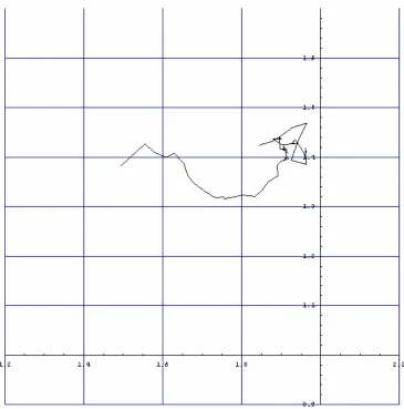
identification system. Our first attempts relied on the manipulation of tracks. A track is created by plotting the mean and the variance of the spectrum of each glottal pulse of a specific utterance, with the mean being the x-axis and the variance the y-axis. We tried two different ways of comparing tracks: Minimum Enclosing Rectangle (MER) and Curvature Scale Space (CSS) images.

These approaches ultimately did not satisfy our requirements; however, the work did lead us to the current approach, so it is worth mentioning in detail. The methods involving the comparison of tracks can be broken down into three discrete steps:

a) Obtain sound sequences consisting of voiced sounds

b) Perform spectral analysis on the sound sequences to create tracks c) Compare Tracks

3.1 OBTAINING SOUND SEQUENCES

First, the recordings of both the known speakers and the unknown speakers are transcribed. Next we search the transcriptions for words or parts or words that are completely voiced – that is, where the vocal chord vibrates throughout. The same voiced segments need to be present in each transcription. Each is extracted and saved in a .wav file. The methodology used for finding a voiced sample is explained in the next chapter.

Because the segments are the same across all speakers, dialectic differences in the

(40)

word “bird” can be a good discriminator between a person from Brooklyn who pronounces the word as “boid” and another person who pronounces it “bird”. Even though the same word is being uttered, the pronunciation is very different, and it therefore differentiates between the two speakers.

3.2 SPECTRAL ANALYSIS FOR TRACK CREATION

Once a sound file has been saved, we then use a Mathematica program to perform spectral analysis on it. The first step is to divide the speech sample into glottal pulse periods, where each period represents the vibration of the vocal chords. The program needs the user to provide a maximum and minimum estimate of twice the samples of the glottal pulse period. Once that is done, the program takes a speech sample (equal in size to the minimum estimate), performs a Fourier Transform on it, and calculates the first four harmonics. A harmonic is an integer factor of the fundamental frequency, which is the inverse of the period length. The four harmonics are then summed and the sum is saved.

The speech sample size is increased by 1 sample and the step is repeated. This will

continue until the speech sample size is equal to the maximum estimate given by the user. The sample size that resulted in the minimum harmonic sum is taken to be the glottal pulse period size.

(41)

an array by sampling the speech in a moving window, shifting the window one sample to the right for each array element. Each element is a speech sample twice the length of the approximation. The program uses the variable k to represent the size of the first

approximation, then it drops the first k-50 elements from the front of the array. Next it searches for the index of the remaining element whose value is the maximum. This index is the second estimate of the glottal pulse period.

Once the glottal pulse periods have been calculated, for each glottal pulse period of N samples, the following will be performed:

• The absolute value of the Fourier Transform of N samples is calculated

• A shift of one sample to the right is done, and the step above is repeated

Once all N Fourier Transforms have been computed, the average Fourier Transform is computed. The cube root of the average is then taken to minimize the effect of the first formant, which is the first peak in the frequency spectrum that has great amplitude, especially in vowels. Then the DC term is dropped, and the resulting transform is interpolated, creating a continuous spectrum from 0 to 4000 Hz [15].

(42)

∫

=

≤

b

a

dx

x

f

b

X

a

P

(

)

(

)

After the conversion, the mean (first moment) and variance (second moment) of the pdf are computed. Then a moment track is created with the first moment of the pdf be the abscissa and the second moment be the ordinate. One such track would look like the following:

(43)

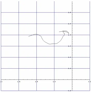
Once the track is created, it is smoothed to reduce any information that is due to noise. The track is smoothed using a cascading filter consisting of three stages: median-5, average-3, and median-3. The median-x stages have each value (except the endpoints) replaced by the median of its original value and the values of the x-1 surrounding points. The average-x stage has each value replaced by the average of its current value and the values of the x-1 surrounding values. The smoothed version of the above track is the following:

(44)

The smoothed track is used to represent a particular speaker uttering a particular

utterance. This track will be compared with tracks from the same user uttering the same utterance and with tracks from different users uttering the same utterance. Next, the tracks will be compared using either the MER or CSS algorithms. Both are explained below.

3.3 TRACK COMPARISON

3.3.1 Minimum Enclosing Rectangle (MER)

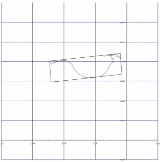
An MER is a rectangle of minimum area that encompasses the whole moment track. The algorithm starts by translating the track to the origin. Then 91 bounding boxes are computed, by starting at 0 degrees and rotating by 1 degree per iteration, up to 90

(45)

Figure 3.3 MER for a smoothed track

To capture the position and orientation of the track, various features of the MER were calculated: the x and y coordinates of the midpoint, the length of the long side of the MER, the minimal x-coordinate, the minimal y-coordinates, the maximal x-coordinate, and the maximal y-coordinate (determined by the four corner points of the MER).

To capture the shape of the track, two additional variables are calculated. Since the spacing and the number of track points depend on the fundamental pitch (a higher

(46)

More specifically, two new curves are made: one curve has a point p of the first moment as the ordinate, and the distance between that point and the point p+1 (or the point following it in such way that the distance is larger than a set threshold) as the abscissa. The abscissa is then normalized in [0,1] and the points are interpolated using a cubic spline. The second curve is calculated the same way, but the points used are the ones in the second moment. Once the curves are enacted, the two shape-based variables are calculated by integrating each curve over the [0,1] interval.

We conducted 2 experiments to test the accuracy of the MER method. The first

experiment was closed-set and used three isolexemic sequences: ayo (as in payola), eya (as in agree about), and owie (as in now we see). Samples of each of the sequences were taken from the speech of ten speakers, five of whose first language was English, and five of whose first language was Spanish, but who have an excellent grasp and pronunciation of English. Each speaker uttered ayo, eya and owie four times to provide the training for the database.

Analysis of Variance (ANOVA) was used to ascertain that the MER and track features explained above were in fact significant. The F-ratio in ANOVA represents the ratio of inter-speaker variation to intra-speaker variation. If the F-ratio is larger than 2.2

(preferably much larger), then the feature is significant in discriminating between speakers. The results of this experiment indicate that all the features described above were actually significant: for ayo, the least significant attribute was the angle of rotation with an F-ratio of 7.66 and the most significant was the quadrature of the second

(47)

angle of rotation with an F-ratio of 2.32, and the most significant one was the maximal y-coordinate with an F-ratio of 57.17. Finally, for owie, the least significant attribute was actually a tie between the long side of the MER and the angle of rotation with an F-ratio of 4.61, and the most significant attribute was the quadrature of the second moment with an F-ratio of 67.49.

After determining the significance of the features, we performed a discriminant analysis using all 30 variables (10 variables per sound, three sounds), and distances were

computed using Mahalanobis Distances, since they account for variances and covariances between variables. The smaller the distance between speakers, the closer these speakers are with respect to the variables used. The smallest distance between speakers was 98, and the largest was 708.

For this (closed-set) experiment, we selected an extra utterance of ayo, eya, and owie for 7 of the 10 speakers, and used that as the testing set. The unknown speaker is identified as one of the known speakers by selecting the known speaker whose distance from the unknown speaker is the smallest. All seven unknown speakers were accurately

identified, with all but one having a distance of less than 100.

(48)

speakers would be incorrectly identified as one of the in-set speakers. Furthermore, one of the in-set speakers would be incorrectly identified as an out-of-set speaker.

These results indicate that even though there is some discrimination using the MER, it would become impossible to have close to a 99% accuracy rate in the open-set case. The open-set case will be the most important case in forensic speaker identification, since the criminal exemplar could be anyone in the world. For that reason, we did not feel that the MER gave us good enough results to use by itself. We then thought about the possibility of using the MER results in conjunction with other methods that would corroborate the variations. One of these other methods is using Curvature Scale Space (CSS) images, which is described below.

3.3.2 Curvature Scale Space Images

Another way to obtain information from the moment track is to represent each track by its corresponding CSS image. A CSS image is a multi-scale organization of the curvature zero-crossings points of the shape of the track as it changes. Curvature is defined as a local measure of how fast a planar contour is turning. Therefore, the CSS image is a good representation of the shape of the track, determining the bend of the track and the

deviation from a straight line as it moves across moment space.

3.3.2.1 CSS Image Creation

A CSS representation of the track is created by following these steps:

(49)

b) The track is convolved with a Gaussian kernel of width

σ

, ranging from 1 to 256. A Gaussian kernel is defined as a kernel with the shape of a Gaussian (normal distribution) curve, mathematically defined as:

2 2 2

2

1 )

,

(

σ

π

σ

t

e

t

g

−

=

As

σ

increases, the kernel function becomes broader and flatter, and as

σ

gets closer to zero, the kernel function becomes narrower and sharper. These changes are because the area under the curve is kept constant.

c) The result of convolving the track with the kernel is a smoother version of the track. As

σ

increases, the track becomes smoother. The curvature of the track, κ , is computed for every value of σ in the following way:

(

) (

)

[

]

2

3 2 2

)

(

)

(

)

(

)

(

)

(

)

(

σ

κ

u u u uu uu u

Y

X

Y

X

Y

X

+

−

=

Where Xu(σ) and Yu(σ) are the convolution of the first derivative with the

x and y-axis, respectively; and Xuu(σ) and Yuu(σ) are the convolution of the

second derivative of the Gaussian kernel with the x and y-axis, respectively.

(50)

point p+1 is negative/positive. When a point is a zero-crossing, it is recorded in a two-dimensional array with the value of the point and the current value of

σ where the zero-crossing was found.

e) Once all zero crossings are found for a particular σ, the value of σ increases by 1, and the curvature calculation is repeated. This is done until there is a σ

value where there are no zero-crossings.

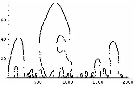
f) Once the σ has been found, the CSS image is constructed by using the two-dimensional array in the following way: the value of the location of the zero-crossing is the ordinate, while the σ value where the zero-crossing was found is the abscissa. One such CSS image would be the following:

Figure 3.4 Example of a CSS image

(51)

3.3.2.2 CSS Image Matching Algorithm

The matching algorithm is a revised version of the algorithm proposed by Mokhtarian, et al. [10] The purpose of the algorithm is to provide a number to indicate how similar two tracks are in terms of curvature. Each CSS image will only be represented by the local maxima, since the longer and deeper a concavity is, the taller the corresponding CSS contour will be. So only the maximum of each CSS image’s contour needs to be

compared to determine if the concavities are the same or not, and hence, how similar the curvatures of two curves are.

The matching algorithm uses a node structure for storage to compare between two CSS images, which we shall call CSS1 and CSS2. Each node contains the following fields:

• CSS1_Point contains one element from the two-dimensional array of CSS1

(which was populated during the image creation, as explained in the section above).

• CSS2_Point also contains one element, but from the two-dimensional array of

CSS2.

• CSS1_Array is a dimensional array containing values from the

two-dimensional array created when CSS1 was created.

• CSS2_Array is a dimensional array containing values from the

two-dimensional array created when CSS2 was created.

• Cost is an integer value which will ultimately contain the cost of the matching

(52)

One node is created with all the fields either set to 0 (for the Cost) or empty (for the other variables). Then the algorithm starts:

a) The largest maximum of CSS1 and CSS2 is found (for each image), and the node’s CSS1_Point and CSS2_Point are populated with those numbers. The Cost field is set to the absolute value of the difference of the σ values of the largest maximum of CSS1 and CSS2.

b) A node is created for each maximum in CSS2 that comes within 80% of the σ

value of the largest maximum of CSS1, where CSS1_point is set to the largest maximum in CSS1, and CSS2_point is set to the maximum that is within 80% of the σ value of CSS1_point. A node is also created for each maximum in CSS1 that comes within 80% of the σ value of the largest maximum in CSS2. In this case, the CSS2_point is set to the largest maximum in CSS2 and CSS1_point is set to the maximum within 80% of the σ value of CSS1_point. This is done to be able to match any considerable possibility so that the matching cost is minimized.

c) For each node created in the previous two steps, two arrays are initialized: CSS1_Array will contain CSS1_point, and CSS2_Array will contain CSS2_point.

(53)

o If there are no maxima left in CSS1 that are not in CSS1_Array, then the

σ-value of the largest CSS2_maximum that is not in CSS2_Array is added to the Cost.

o If there are no maxima left in CSS2 that are not in CSS2_Array, then the

σ-value of the largest CSS1_maximum that is not in CSS1_Array is added to the Cost.

o If the location difference between the two maxima found is within 0.2, then the absolute value of the σ-value difference is added to the cost.

o Otherwise, the σ-value of the CSS1 maximum found is added to the cost.

The CSS1_Array and CSS2_Array are also both updated by adding the maxima found in this step.

e) The current lowest cost node is selected. If there are any maxima left in either CSS1 or CSS2 that are not in the CSS1_Array or CSS2_Array, respectively, then the node is expanded as explained in the previous step. If all the maxima are contained in the CSS1_Array and CSS2_Array, then the Cost variable for that node is returned as the lowest matching cost between the two CSS images.

f) CSS1 and CSS2 are swapped, and the algorithm is repeated to find the lowest cost with images swapped.

(54)

3.3.2.3 CSS Image Matching Results

We conducted another closed-set experiment to determine the effectiveness of the CSS images in discriminating between tracks. We used the same samples as we had in the closed-set MER experiment: the same ten speakers uttering ayo, eya, and owie 5 times, selecting the middle three samples of each utterance. The smaller the matching cost of two CSS images are, the more similar the two tracks they represent are with each other. Below is a table with the results of the experiment:

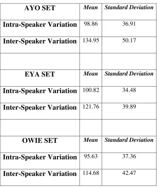
Table 3.1. Results for the Closed-Set CSS Image Experiments with 10 Speakers

AYO SET

Mean Standard Deviation

Intra-Speaker Variation

98.86 36.91

Inter-Speaker Variation

134.95 50.17

EYA SET

Intra-Speaker Variation

100.82 34.48

Inter-Speaker Variation

121.76 39.89

OWIE SET

Intra-Speaker Variation

95.63 37.36

(55)

The mean for the Intra-Speaker variation was calculated by adding all the same-speaker CSS images’ matching costs for a single utterance at a time and then the resulting cost was divided by the different combinations of same-speaker CSS images’ matching costs. This calculation was done for all three different sounds. The inter-speaker variation mean was found the same way, except having all the combinations of different-speaker CSS images’ matching costs.

As can be seen in the table above, the mean for the intra-speaker variation for all three sounds was smaller than for the inter-speaker variation, indicating that using the CSS images as a discriminating factor provides lower intra-speaker than inter-speaker variation. However, the standard deviations for all the intra-speaker variations are very high, indicating an unacceptably wide spread in the results. Since these results occurred from the closed-set experiment, we did not need to conduct an open-set experiment (which would be expected to produce worse results). The only reason to do an open-set experiment would have been if the closed-set experiment had provided optimal results: a lower intra-speaker than inter-speaker variation mean with a small standard deviation.

(56)

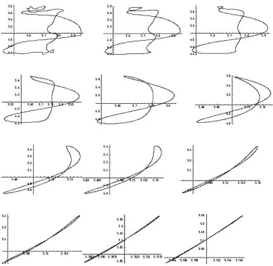
a undesirable result in the evolution of the track. One example is the track evolution presented below:

Figure 3.5 Evolution of a Track Convolved with a Gaussian kernel

(57)

infinitely and cannot be used for the experiment. This of course causes a problem because some of the data is wasted.

(58)

CHAPTER 4: CURRENT METHOD

Of the track-based methods described in chapter 3, the most promising was the MER method, which we described in [15]. We have iterated through several changes to the 3-step MER method to arrive at the current approach, which we call semi-automatic speaker identification. The name "Semi-automatic" is given because it is a part human, part machine speaker identification system. Throughout the process of designing and implementing this system, we had the goal of adhering to these requirements:

• The system shall produce a lower intra-speaker than inter-speaker

variation: This requirement is the most important, since a speaker will never

utter the same utterance the same way. There is always variation between different utterances from one speaker, even when the utterances are the same words. Any speaker identification system should account for this expected intra-speaker variation.

• The system shall be at least 99% accurate: This is an important

requirement for use in the court system. If our method can be shown to have 99% or more accuracy, then the results are more valuable as evidence in a court case.

• The system shall determine the unknown speaker in both the open-set

and closed-set situations: Closed-set speaker identification is appropriate for

(59)

as open-set speaker ID in order to identify a criminal, it is very important to be able to establish that none of the suspects matches the criminal, so that no innocent person is convicted of a crime.

• The system shall be text-independent: In forensic speaker identification, the

speech evidence encountered will almost always be different from the speech given by the suspects. Therefore, a useful speaker identification system will need to be text-independent.

After publishing the MER method we ultimately realized that it failed to meet our requirements. We knew from the experiments that the tracks and the information they represented were in fact important in discriminating between speakers. The problem was that the moment space did not specifically take into account all the discriminating

information the utterances had. Also, some of the glottal pulses may not provide as much information as others.

The following sections summarize the changes we made step-by-step as we progressed from the initial method to the current method.

4.1 METHOD MODIFICATION: ISOCHUNKS

(60)

The second reason is that whenever a new known speaker is added to the set of suspects, most, if not all, of the isochunks selected for the other known speakers need to appear in the new known speaker’s speech sample. The number of different isochunks per speaker makes the discrimination more robust, so there is a need to have as many isochunks as possible appear in each known speaker’s speech sample.

Each isochunk is extracted manually by listening to each speech sample, transcribing it, pinpointing the isochunk location, and finally listening to the sections where the

isochunks appear, and saving each isochunk in its own .wav file with a 44.1 KHz sampling frequency. Choosing isochunks became the first step in our evolved method.

4.2 METHOD ADDITION: SEGMENTOR CREATION

An assumption that has not been mentioned until this point is that our method will only work with voiced sounds. Voiced sounds occur when there are vibrations of the vocal chords, while in voiceless sounds, there is no vibration of the vocal chords present. Since we rely on information contained in glottal pulses (vibrations), we need to use samples where the vocal chords are vibrating. One word or utterance can contain both voiced and voiceless sounds. So in choosing isochunks, it is often not possible to select an utterance that is 100% voiced. Because of this, we needed to add a step to our method that would differentiate between voiced, voiceless, and silence sounds.

(61)

using the first four harmonics and the autocorrelation estimation as explained in section 3.2.)

The segmentor begins with one isochunk. It uses a window of 900 samples at a time of each isochunk, accounting for an approximation of twice the size of a glottal pulse period. It then calculates the Fourier Transform for this window, and stores only the first 100 harmonics of the resulting transform. The 100 number is used based on previous research by the speech research group at North Carolina State University. After the first 100 harmonics, they have found there is no significant amplitude that would modify either the glottal pulse estimation or the segment identification.

The segmentor then calculates the Fourier Transform of the first 100 harmonics. This results in a curve with two maxima. The first maximum will be found in the DC term, which represents the total energy of the spectral envelope. The spectral envelope is the boundary envelope that encompasses the whole spectrum. The other maximum is found in the second half of the curve (points 25-50), and it represents the energy of the

harmonic peaks of the first transform, and it is the one of interest for our method.

If the energy amplitude represented by this half is below a set threshold, the segment is considered voiceless, since the amplitude is so small that it will not help in the

(62)

a) A new window is calculated in the following way: the position of the second-half maximum is multiplied by the current window size (which is initialized at 900)

b) Both Fourier Transforms explained above are again calculated, but this time using the shrunken window. The second fourier transform is analyzed, and the second-half maximum is found.

c) The previous two steps are repeated until one of two requirements are met:

i. The shrunken window size is less than 200. If this is the case, the segment is considered voiceless.

ii. The second-half maximum’s position is at 50, the farthest position in the transform. If this is the case, then the current size of the shrunk window provides a very good estimate of the glottal pulse period.

Once this is done, 100 samples are removed from the speech signal, a window of 900 samples is selected, and the algorithm is repeated again. This repetition stops once there are less than 900 samples remaining in the speech sample.

(63)

sample window. The glottal pulse period estimates of the selected sample window are used for the rest of the method. In a later step the glottal pulse estimates found by the segmentor are compared to those found by the minimum 4 harmonics and autocorrelation methods as a double-check. In our testing to date the segmentor has always given reasonable (usable) estimates.

At this point, step 1 of our final method is choosing isochunks and step 2 is running the segmentor.

4.3 METHOD DECISION: WILL DIFFERENTIATION PROVIDE THE

NECESSARY DISCRIMINATION?

After the segmentor was completed, the next problem to tackle was how the spectrum information would be used to discriminate between speakers. Our original spectral analysis step (explained in section 3.2) still provided the information needed to create the discriminating spectra. In the final method, the spectrum is calculated the same way, except now the glottal pulse period estimation, as long as it is within 45 samples of both the autocorrelation estimation and the odd harmonics estimation, is taken to be the one given by the segmentor.

Semi-Automatic Forensic Speaker Identification

TABLE OF CONTENTS

LIST OF TABLES

LIST OF FIGURES

CHAPTER 1: INTRODUCTION

1.1 TERMINOLOGY

1.2 THESIS OUTLINE

CHAPTER 2: RELATED WORK

2.1 NEURAL NETWORKS

2.2 VECTOR QUANTIZATION

L

k

C

X

d

T

e

=

∑

≤

≤

1

)],

,

(

[

min

1

2.3 GAUSSIAN MIXTURE MODEL

)

(

)

|

(

x

b

p

x

p

∑

=

λ

|

|

)

2

(

1

)

(

x

e

b

π

Σ

=

µ

)

|

(

log

max

arg

~

∑

=

p

x

λ

λ

λ

2.4 EIGENVOICES

2.5 WAVELETS













−