Classification and performance evaluation
using data mining algorithms
Vaibhav P. Vasani1, Rajendra D. Gawali 2
Lecturer, Information Technology, PVPP’S Manohar Phalke Polytechnic, Mumbai, Maharashtra, India 1
Assistant Professor, Computer Engineering, Lokmanya Tilak College of engineering, Navi Mumbai, Maharashtra, India 2
Abstract:In this paper, classification of the data collected from students of polytechnic institute has been discussed. This data is pre-processed to remove unwanted and less meaningful attributes. These students are then classified into different categories like brilliant, average, weak using decision tree and naïve Bayesian algorithms. The processing is done using WEKA data mining tool. This paper also compares results of classification with respect to different performance parameters.
Keywords: Classification; data mining; decision tree algorithm; educational data mining; Naïve Bayesian algorithm; WEKA; education; confusion matrix; margin curves; accuracy; true positive rate; false positive rate; precision; threshold curves.
I. INTRODUCTION
Different areas of research in educational data mining are analysis and visualization of data, recommendations for students, student modeling, detecting undesirable student behaviour, grouping of students, social network analysis, developing concept maps, constructing courseware, planning and scheduling and predicting student’s performance.
II. LITERATURE SURVEY
Educational data mining (EDM) is a field that exploits machine-learning, statistical and data-mining algorithms over the different types of educational data. Its main objective is to analyse data in order to resolve educational research issues. EDM is concerned with developing methods to explore the unique types of data in educational settings and, using these methods, to better understand students and the settings in which they learn. This data helps to understand learners and learning and to develop computational approaches that combine data and knowledge to transform practice to benefit learners [1] [4] [5].
The objective of prediction is to estimate the unknown value of a variable that describes the student. Prediction of performance, knowledge, score, or mark is done. This value can be numerical/continuous value (regression task) or categorical/discrete value (classification task). Regression analysis finds the relationship between a dependent variable and one or more independent variables. In classification individual items are placed into groups based on quantitative information regarding one or more characteristics inherent in the items and based on a training set of previously labeled items. For Prediction techniques used like neural networks, Bayesian networks, rule-based systems, regression, and correlation analysis is also. Different types of neural-network models have been used to predict final student grades (using back-propagation and feed-forward neural networks). A candidate being considered for admission into the university (using multilayer perceptron topology), Bayesian networks have been used to predict student applicant performance [1] [2] [3].
III. IMPLEMENTATION
One of the popular data mining tools is WEKA (Waikato Environment for Knowledge Analysis). Since this is open source tool and supports many data mining algorithms, this has been used for pre-processing and classification of student data.
WEKA 3.6.6 has been used to classify the students using decision tree and Naïve Bayesian algorithms.
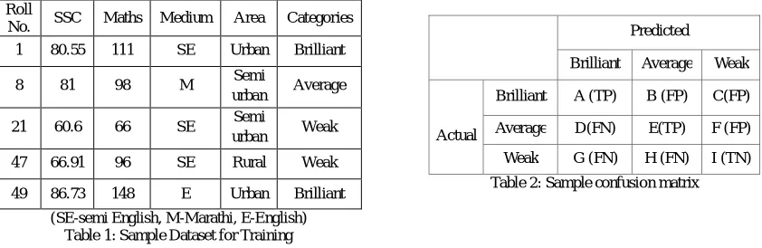
Sample dataset: Here data for classification has been collected from 220 students of private polytechnic institute. To analyse dataset, attributes considered are SSC marks (percentages), maths (marks in mathematics), medium (language of instruction), and area (place of residence). Roll numbers were considered initially for row identification. But they were removed during pre-processing of data, as they were generating errors in calculation. The sample dataset is shown in table 1.
Roll
No. SSC Maths Medium Area Categories 1 80.55 111 SE Urban Brilliant
8 81 98 M Semi
urban Average
21 60.6 66 SE Semi
urban Weak
47 66.91 96 SE Rural Weak
49 86.73 148 E Urban Brilliant (SE-semi English, M-Marathi, E-English)
Table 1: Sample Dataset for Training
Predicted
Brilliant Average Weak
Actual
Brilliant A (TP) B (FP) C(FP)
Average D(FN) E(TP) F (FP)
Weak G (FN) H (FN) I (TN)
Table 2: Sample confusion matrix
Accuracy/error rate estimation: Errors in the classification techniques can be considered as incorrect classification of instances. These errors refer to overall performance of the model or the algorithm.
Following table 2 shows the confusion matrix where rows representing the actual classes and the columns the predicted classes such as brilliant, average and weak.
Student in the dataset may belong to any one of the category such as A (correct prediction, true positive), B (incorrect prediction, false negative), C (incorrect prediction, false negative), D (incorrect prediction, false positive), E (correct prediction, true positive), F (incorrect prediction, false negative), G (incorrect prediction, false positive), H (incorrect prediction, false positive) and I (correct prediction, true negative).
Accuracy which is the ratio of the number of incorrectly classified instances to the total number of examined instances can be calculated as
True Positive Rate (TPR) or recall is the ratio of positive instances that were correctly identified to the total number of actual positive instances, can be calculated as
, and
False Positive Rate (FPR) is the ratio of negative instances that were incorrectly classified as positive to the total number of negative instances and can be calculated as
, And
Precision is the ratio of predicted correctly to the total predicted and calculated as
IV. RESULTS AND DISCUSSION
Table 3 compares results of Decision tree (J48) and Naïve Bayesian Algorithms with respect to different performance criteria.
Criteria J48 algorithm
(Decision Tree) Naïve Bayesian algorithm
Correctly Classified Instances 211/220
(95.9091 %) 190/220 (86.3636 %)
Incorrectly Classified Instances 009/220
(04.0909 %) 30/220 (13.6364 %)
Kappa statistic 0.9366 0.7855
Mean absolute Error 0.0482 0.1108
Root mean squared error 0.1675 0.2608
Relative absolute error 11.2272 % 25.8011 %
Root relative squared error 36.1544 % 56.3154 %
Table 3: Comparison of algorithmic performance
Results of J48 (Decision Tree) Algorithm: Accuracy measures and confusion matrix for each class using J48 algorithm are as shown in table 4 and 5 below,
Class TP Rate
FP
Rate Precision Recall F-Measure
ROC Area
Brilliant 0.957 0.031 0.957 0.957 0.957 0.957
Average 0.938 0.021 0.962 0.938 0.949 0.962
Weak 1.000 0.012 0.959 1.00 0.979 0.990
Weighted
Avg. 0.959 0.024 0.959 0.959 0.959 0.966 Table 4: Accuracy for J48 (Decision Tree) Algorithm
A B C <== Classified as
89 3 1 a = Brilliant
4 75 1 b = Average
0 0 47 c = Weak
Table 5: Confusion Matrix for J48 Algorithm
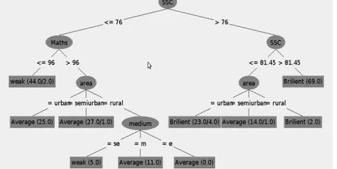
Figure 1 shows the decision tree after the training the system and gives classification of data into brilliant, average, and weak.
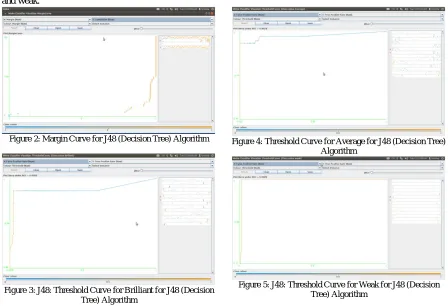
Figure 2: Margin Curve for J48 (Decision Tree) Algorithm
Figure 3: J48: Threshold Curve for Brilliant for J48 (Decision Tree) Algorithm
Figure 4: Threshold Curve for Average for J48 (Decision Tree) Algorithm
Figure 5: J48: Threshold Curve for Weak for J48 (Decision Tree) Algorithm
Results of Naïve Bayesian Algorithm: The probabilities of classes found using naïve Bayesian algorithm are brilliant (0.42), average (0.36) and weak (0.22).
Accuracy measures and confusion matrix for each class using naïve Bayesian algorithm are as shown in table 6 and 7, Confusion Matrix for J48 Algorithm in table 7 shows the classification of 220 students in dataset into different classes.
Class TP Rate
FP Rate
Precis ion
Recal l
F-Measure
ROC Area
Brilliant 0.914 0.087 0.885 0.914 0.899 0.975
Average 0.863 0.129 0.793 0.863 0.826 0.938 Weak 0.766 0.006 0.973 0.766 0.857 0.986 Weighte
d Avg.
0.864 0.085 0.871 0.864 0.864 0.964
Table 6: Accuracy for Naïve Bayesian Algorithm
A B C <== Classified as 87 7 1 a = Brilliant 11 69 0 b = Average 0 11 36 c = Weak
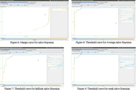
Figure 6: Margin curve for naïve Bayesian
Figure 7: Threshold curve for brilliant naïve Bayesian
Figure 8: Threshold curve for Average naïve Bayesian
Figure 9: Threshold curve for weak naïve Bayesian
The margin curves of J48-Decision tree and Bayesian classification algorithms are shown in figure 2 and 6 respectively. The margin curve prints the cumulative frequency of the difference of actual class probability and the highest probability predicted for other classes (so, for a single class, if it is predicted to be positive with probability p, the margin is p-(1-p) =2p-1). The negative values denote classification errors, meaning that the dominant class is not the correct one.
The figure 2 depicts, the majority of instances are correctly classified by J48 decision tree model, since they are centralized in the area of probability one (the right part of the graph). On the other hand, the classified instances of Naïve Bayesian algorithm (figure 6) are not concentrated in that area, revealing a significant deviation.
The visualized threshold curves show (figures 3, 4 & 5 for J48-decision tree algorithm and figure 7, 8 & 9 for Naïve Bayesian algorithm) the effect of varying the probability threshold above which an instance is assigned to that class. It represents that how data is perfectly classified as if curve is more towards the left corner of graph. It proves that all data is perfectly classified in all three categories viz. Brilliant, average and weak.
V. CONCLUSION
Students in dataset are classifieds into brilliant, average and weak classes on the basis of their SSC marks, marks of mathematics, area of residence, medium of instruction.
The result of classification can be used to take remedial actions on students learning process. This study shows more attention should be given to improve basic fundamentals in mathematics and language. This can be improved with help of tutorials, training and seminars for weaker sections of the students. Also it is observed that students from remote or rural lack in confidence which results in lower grades in examination. Their confidence level may be raised by mentoring them by faculties as well as through the motivational lectures.
The overall improvement in student performance may help them to succeed in academics as well as industrial/professional skills.
After comparing results of both algorithms, it is also observed that Decision tree (J48) gives better result than Naive Bayesian algorithm in terms of accuracy in classifying the data.
REFERENCES
[1] Cristobal Romero, Member, IEEE, and Sebastian Ventura, Senior Member, IEEE “Educational Data Mining: A Review of the State of the Art”, IEEE November 2010
[2] Jiawei Han, Micheline Kamber, “Data Mining”, Second Edition, Elsevier, 2008
[3] A. B. M. Shawkat Ali, Saleh A. Wasimi, “Data Mining: Methods and techniques” Cengage Learning, 2009
[4] Yafei Sun, Zhishu Li, Lei Zhang ; Shuxiong Qiu, Yang Chen, “Evaluating Data Mining Tools for Authentic Emotion Classification”, Intelligent Computation Technology and Automation (ICICTA), 2010 International IEEE Conference, Page(s): 228 - 232
[5] Weka manual, Free available, site: www.cs.waikato.ac.nz/ml/weka/index_documentation.htm
BIOGRAPHY
Vaibhav P. Vasani is working with PVPP’S Manohar Phalke Polytechnic, Sion, and Mumbai, India and also he is pursuing Masters of Engineering in Computer Engineering at Lokmanya Tilak College of Engineering, Navi Mumbai, India. His area of research is Data base and Data Mining.