Process control parameters for Skipjack tuna (Katsuwonas pelamis) precooking

(1)

ABSTRACT

WEBB, ELIZABETH LYNN. Process control parameters for Skipjack tuna (Katsuwonas pelamis) precooking. (Under the direction of S. Andrew Hale).

The purpose of this research was to define the critical process control parameters that influence texture and yield for the precook unit operation in the commercial canning of Skipjack tuna. To accomplish this goal, the impact of precook temperature and time combinations on the Instrumental Texture Profile Analysis (ITPA) texture parameters, protein state, weight loss, and moisture content of hydrothermally treated tuna loin meat was investigated. It was found that temperature was the primary influence for all ITPA parameters, however time influenced texture when samples were held at 55°C. Auto proteolysis was suspected at this temperature, as some ITPA parameters declined with increased time.

Data from small steamed and small hydrothermally treated samples were compared with data from whole steamed fish to ascertain whether small sample results could be extrapolated to data from whole precooked fish. Weight loss, moisture content, and ITPA values reacted similarly, regardless of experiment method. For all treatments, weight loss and moisture content decreased with increased temperature, and hardness, instantaneous springiness, and retarded springiness increased with increased

temperature. Cohesiveness did not vary with temperature. Linear conversion equations were written to predict texture, weight loss, and moisture content results of whole

precooked fish from small steamed and small hydrothermal samples.

(2)

(3)

P

R

O

C

E

S

C

O

N

T

R

O

L

P

A

R

A

M

E

T

E

R

S

F

O

R

S

K

I

P

J

A

C

K

T

U

N

A

(

K

a

t

s

u

w

o

n

a

s

p

e

l

a

m

i

s

)

P

R

E

C

O

K

I

N

G

by

Elizabeth Lynn Webb

A dissertation submitted to the Graduate Faculty of North Carolina State University

in partial fulfillment of the requirements for the Degree of

Doctor of Philosophy

BIOLOGICAL AND AGRICULTURAL ENGINEERING

Raleigh

2003

APPROVED BY

(4)

DEDICATION

(5)

BIOGRAPHY

Elizabeth Webb was born in Ocala, Florida and grew up nearby in the small towns of Ocklawaha and East Lake Weir. She is a ninth generation native Floridian, and the oldest of four daughters of Ricki and Jack Webb. Her roots are in oranges,

grapefruit, and tangerines, not tuna, as she is the fifth generation of her family to work in citrus. She spent her free time during her youth enjoying sports, horseback riding, hunting, fishing, occasional waterskiing, and other tomboyish activities.

Elizabeth received her Bachelors in Agricultural Engineering from the University of Florida, Gainesville, Florida in September 1994. After graduating, she was employed for two years as a process engineer with Brown Citrus Systems in Winter Haven Florida where she provided technical advice and engineering solutions to domestic and

international citrus processing plants. She earned her Masters of Science degree in engineering by studying the graduate Chemical Engineering curriculum from the University of South Florida, Tampa, Florida in May 1997. Her thesis was titled

(6)

ACKNOWLEDGEMENTS

I thank my family, Will, Jack, and Willie, for their patience and sacrifices during all the time I spent on this work. Thanks also to Dr. Andy Hale for the latitude to pursue my research, the guidance when things went bad, and his kindness for understanding life. I am indebted to Dr. Brian Farkas, who has given me much encouragement and needed direction throughout my doctoral endeavours. My gratitude goes to Dr. Tyre C. Lanier for sharing his wealth of seafood knowledge with me. I also appreciate Dr. Kevin Keener and Dr. Jim Young for their input during my studies.

My work is only one part of a research project on tuna and tuna processing. I owe the rest of The Tuna Group, as we were collectively called, a big thank you for their group spirit and willingness to help – kudos to Jon Bell, Janet Zhang, Nicola Stagg, Heather Stewart, and Penny Amato. I especially thank Tim Seaboch for his help and camaraderie throughout my stay in North Carolina, some of which was imparted during the many, many experiments I ran in 117.

I would like to recognize StarKist Seafoods and the USDA for providing funds and support for my research project. I want to thank two StarKist employees in particular - Jaime Citron and Joe Emmer - for coordinating the shipment of the all the frozen, cannery grade tuna used in my research.

(7)

LIST OF TABLES

3.0 MANUSCRIPT 1

Table 1 R2 and a values from ANOVA analysis, type III sum of squares results for the effect of temperature, time, weight loss, and moisture content on ITPA parameters of Skipjack tuna light loin

meat for all temperature treatments ...72 Table 2 R2 and a values from Pearson correlation analysis results to

examine relationships between temperature, time, weight loss, and moisture content on ITPA parameters of Skipjack tuna

light loin meat...73 Table 3 R2 and a values from Pearson correlation analysis results to

examine the relationships between ITPA parameters of Skipjack tuna light loin meat...73 4.0 MANUSCRIPT 2

Table 1 P values from ANOVA type III sum of squares for the effect of experiment treatment on weight loss, moisture content, and

ITPA parameters of Skipjack tuna light loin meat ...102 Table 2 P values from ANOVA type III sum of squares for the effect of

temperature, weight loss, and moisture loss on ITPA parameters of Skipjack tuna light loin meat grouped by

experiment treatment...102 Table 3 Linear prediction equations of weight loss and moisture content

for temperature (°C) as the independent variable for Skipjack tuna small steamed, whole steamed, and small hydrothermal

samples...103 Table 4 Linear prediction equations of listed ITPA variables for temperature

(°C) as the independent variable for Skipjack tuna small steamed, whole steamed, and small hydrothermal samples...107 Table 5 Linear prediction equations for listed dependent variables for whole

fish as a function of small steamed and small hydrothermal values for Skipjack tuna samples...117 5.0 MANUSCRIPT 3

Table 1 MLR, neural network, and fuzzy logic R2 and RMSE for time,

(11)

LIST OF FIGURES

2.0 LITERATURE REVIEW

Figure 1 Skipjack tuna (Katsuwonus pelamis) ...5

Figure 2 Skipjack tuna range ...5

Figure 3 Diagram of mammalian muscle tissue ...7

Figure 4 Skipjack tuna muscle structure...8

Figure 5 Tuna canning diagram ...10

Figure 6 Cross section of a Skipjack tuna showing upper and lower loins, dark meat, backbone, viscera cavity, and belly meat ...11

Figure 7 DSC thermogram of raw beef muscle scanned at 10°C/min with denaturation peaks at 55°C, 66°C, and 79°C ...14

Figure 8 Hypothetical ITPA curve ...19

Figure 9 The geometric shape (a) and membership function (b) for a square ...27

Figure 10 Nonlinear relationship of heat and red color for a metal rod...29

Figure 11 A fuzzy nonlinear relation matching regions in the input space to regions in the output space for amount of heat applied to a rod and the resulting red color ...30

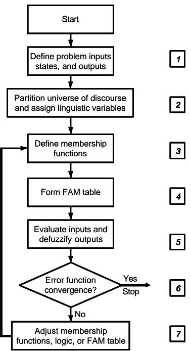
Figure 12 Pseudocode for a fuzzy logic system, using an iterative procedure adjust membership functions, logic, and FAM table ...30

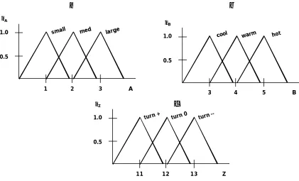
Figure 13 Membership functions for sushi wrap batch size (a), oven temperature (b), and thermostat adjustment (c) ...33

Figure 14 FAM table showing fuzzy output (a) and crisp output (b) for thermostat setting ...34

(12)

Figure 18 Single neuron consisting of input p, weight w, bias b, and

output a ...39 Figure 19 Hard limit (hardlim), pure linear (purelin), and log sigmoid (logsig)

transfer functions ...40 Figure 20 Neural network consisting of an input layer of two nodes, a hidden

layer of four nodes, and an output layer of one node. Bias nodes are not shown ...41 Figure 21 A representation of the multidimensional weight plane for a

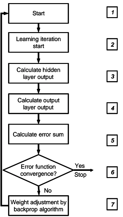
hypothetical problem with a global minimum solution...43 Figure 22 Pseudocode for neural network with backpropagation algorithm,

using early stopping technique ...46 Figure 23 Neural network example with one input, two log sigmoid neurons

in one hidden layer, and one linear neuron in the output layer ...47

Figure 1 Raw Skipjack tuna DSC thermogram at 10°C/min scan rate showing peak I, peak II, and peak III protein denaturation

peaks...69 Figure 2 DSC thermograms at 10°C/min scan rate of Skipjack tuna light

loin muscle after 40°C, 55°C, and 70°C hydrothermal treatments ...70 Figure 3 Amount of protein denatured versus time as measured

by enthalpy changes from DSC thermograms of Skipjack tuna light loin meat muscle proteins after 40°C, 55°C, and 70°C

hydrothermal treatments...71 Figure 4 ITPA hardness versus time for Skipjack tuna light loin meat at

different hydrothermal treatment temperatures...75 Figure 5 ITPA cohesiveness versus time for Skipjack tuna light loin meat at

different hydrothermal treatment temperatures...76 Figure 6 ITPA instantaneous springiness versus time for Skipjack tuna

light loin meat at different hydrothermal treatment temperatures ...77 Figure 7 ITPA retarded springiness versus time for Skipjack tuna light

loin meat at different hydrothermal treatment temperatures...78 Figure 8 Ratio of ITPA retarded to instantaneous springiness versus

time for Skipjack tuna light loin meat at different hydrothermal

(13)

Figure 9 Weight loss versus time for Skipjack tuna light loin meat at

different hydrothermal treatment temperatures...84 Figure 10 Moisture content versus time for Skipjack tuna light loin meat

at different hydrothermal treatment temperatures ...85

Figure 1 Tuna processing unit operation diagram ...92 Figure 2 Tuna precooking and canning process...93 Figure 3 Weight loss versus temperature for Skipjack tuna light loin meat

small steamed, whole steamed, and small hydrothermal cooked samples...104 Figure 4 Moisture content versus temperature for Skipjack tuna light loin

meat small steamed, whole steamed, and small hydrothermal

cooked samples...105 Figure 5 ITPA hardness versus temperature for Skipjack tuna light loin

meat small steamed, whole steamed, and small hydrothermal

cooked samples...108 Figure 6 Compressive strength versus temperature for Skipjack tuna light

loin meat small steamed, whole steamed, and small hydrothermal cooked samples...109 Figure 7 Cohesiveness versus temperature for Skipjack tuna light loin meat

small steamed, whole steamed, and small hydrothermal cooked samples...110 Figure 8 Instantaneous springiness versus temperature for Skipjack tuna

light loin meat small steamed, whole fish, and small hydrothermal cooked samples...111 Figure 9 Retarded springiness versus temperature for Skipjack tuna light

loin meat small steamed, whole fish, and small hydrothermal

cooked samples...112

Figure 1 Fuzzy logic model input (left) and output (right) membership

(14)

Figure 3 Predicted versus actual cook time for multiple linear regression, fuzzy logic, and neural network models ...132 Figure 4 Predicted versus actual weight loss for multiple linear regression,

fuzzy logic, and neural network models ...133 Figure 5 Predicted versus actual edible weight for multiple linear regression,

fuzzy logic, and neural network models ...134 Figure 6 Predicted versus actual friability for multiple linear regression,

(15)

1.0 INTRODUCTION

Today, as is the trend with most mass produced, consumable agricultural products, canned tuna has changed from a high profit margin product to a commodity product. In the commodity product business model, several ways exist for a company to remain profitable, including bulk processing, overhead reduction, and decreased raw product waste. To bulk process, a plant must increase production volume while

maintaining the same, or slightly elevated, fixed costs. To use this strategy, food plants can increase throughput while maintaining the same amount of processing machinery, or produce more product in the same amount of production time. Reduced overhead, for most processors, means a reduced workforce and more plant automation. For

inordinately high labor markets, some companies relocate their entire processing facility to a region with less expensive labor costs. A processor can also decrease the amount of wasted raw material used to make a finished product to increase profit.

The tuna industry has already learned the lesson of “running volume”, as processing plants currently exist which turn out millions of cans of tuna per day (Bell, 2000). They have also learned the lesson of overhead reduction through workforce relocation – one example is StarKist tuna’s closing of the Mayaguez, Puerto Rico plant due to high labor costs. The tuna industry’s profit margin has been adversely affected by the high cost of fish; therefore decreased raw product waste translates into increased profit.

(16)

in machinery and worker training (DeSilva, 1992), and undefined process variables which relate to controllable parameters.

Canned tuna is heated twice during processing – once to change the meat texture for hand cleaning of the whole fish, and again during canning to achieve a commercially sterile product. The first heating, or precook, directly impacts a cannery’s profit, as it is the single biggest impact on final product quality and yield (Wheaton and Lawson, 1985; Lassen, 1965). Mistakes made during precook cause yield loss by either unnecessary water loss or undesirable texture changes that cause edible meat loss. A complicating factor during precook is the natural variation of the raw product. Cooked tuna can also suffer from mushy texture after precooking, called mushy tuna syndrome (MTS). MTS is thought to be caused by auto proteolytic enzymes which can be active in the precook temperature range (Stagg, 1999). MTS decreases yield, as light to moderately MTS affected fish are difficult to clean, and fish severely affected by MTS are not suited for canning. The ability to control the precook unit operation would help processors reduce raw product waste and increase profits.

The ultimate goal of this research was to control the canned tuna process for a more predictable yield. To achieve this goal, critical process control parameters needed to be defined for the precook unit operation, as the precook step is the single biggest influence on plant yield. The purpose of this work was to –

• Define the influence of temperature and time, using ranges seen in commercial processing, on texture changes of precooked tuna

• Investigate whether texture degradation and yield reduction occurs at a certain temperature during precooking

• Investigate the effect of temperature and time on tuna mass and moisture changes

(17)

• Model the outcome of final temperature and fish size on cook time, weight loss, edible weight, and friability in whole fish.

• Learn how to manipulate process control parameters to achieve maximum yield while minimizing texture degradation and friability

1.1 REFERENCES

Bell, J.W., 2000. Liquid mass transport in Skipjack tuna muscle (Katsuwonas pelamis) during canned tuna processes [PhD dissertation]. North Carolina State

University, Raleigh, NC.

Choudhury, G. S., and Bublitz, C. G., 1997. Computer based controls in the fish processing industry. Ch 19 in Computerized Control Systems in the Food Industry, G. S. Mittal, Ed. Marcel Dekker, Inc., New York, NY.

DeSilva, C. W., 1992. Research laboratory for fish processing automation. Robotics and Computer Integrated Manufacturing 9 (1) p 49-60.

Finch, R., 1963. The tuna industry. Ch 7 in Industrial Fishery Technology, M. E. Stansby and J. A. Dassow, Eds. Reinhold Publishing Corp., New York. Horner, W. F. A., 1992. Canning fish and fish products. Ch 5 in Fish Processing

Technology, G. M. Hall, Ed. Blackie Academic and Professional, published in North American by VCH Publishers, New York, NY.

Lassen, Sven 1965. Tuna Canning and the Preservation of the Raw Material through Brine Refrigeration. Ch. 4 in Fish as Food, v 4, part 2, G. Borgstrom (Ed.) p. 207-245, Academic Press, New York and London.

Stagg N. 1999. Response of Skipjack tuna muscle protein to thermal processing [MSc thesis]. Raleigh NC: North Carolina State University. 128 p.

(18)

2.0 LITERATURE REVIEW

2.1 Skipjack tuna

Tuna was first canned in 1903, when a disastrous sardine catch forced Mr. A. P. Halfhill of San Pedro, California to search for alternate fish to preserve in an effort to keep his cannery afloat (Finch, 1963). Fourteen species of tuna can be legally canned in accordance with the 1998 Code of Federal Regulations, but canned tuna sold in the United States primarily consists of light meat harvested from Bluefin, Albacore,

Yellowfin, or Skipjack. Skipjack tuna (Katsuwonus pelamis) has become the most popular commercially fished tuna, and currently comprise fifty percent of the worlds catch (Wheaton and Lawson, 1985; Gardieff, 2003; Joseph, 2003). Skipjack also represent the majority of meat canned for chunk light tuna (Bell, 1998).

Skipjack (Figure 1) is epipelagic, inhabiting waters with temperature ranges of 14.7°C to 30°C, and are distributed circumtropically, however also occur along the European coast and the North Sea (Figure 2). Skipjacks tend to school, sometimes with other tuna species. Schooling frequently occurs under a drifting object, or larger marine animals such as whales or sharks. Skipjack often school by size, as smaller fish might not be able to maintain top speeds achieved by larger fish. The maximum

(19)

Figure 1 Skipjack tuna (Katsuwonus pelamis) (Collette and Nauen, 1983).

Figure 2 Skipjack tuna range, in red (Bester, 2003).

2.2 Mammal and fish muscle similarities and differences

2.2.1 Mammalian muscle structure and composition

(20)

consists of long, cylindrical cells called myofibers, surrounded by collagen and elastin fibers, which are located in the extracellular space surrounding the myofibers. One myofiber consists of many myofibrils. Myofibrils consist of thick (15 nm diameter) and thin (6-8 nm diameter) filaments. Myosin is the primary component of thick filaments, while actin, tropomyosin, and troponin are the primary proteins of the thin filaments. Myosin and actin are the primary structural proteins for all meat (Greaser, 1991). The sarcoplasmic proteins, mainly globular, soluble proteins found in extracellular fluid, include myoglobin, hemoglobin, globulins, albumins, and various enzymes. Stroma proteins, collagen and elastin, surround the myofibers, and are less soluble than sarcoplasmic proteins (Venugopal and Shahidi, 1996).

(21)

Figure 3 Diagram of mammalian muscle tissue (Greaser, 1991).

2.2.2 Fish and Skipjack tuna muscle structure and composition

Fish in general have roughly the same composition as beef, although raw Skipjack tuna has less water and more protein - approximately 71.7% water, 25.9% protein, and 0.6% fat (Venugopal and Shahidi, 1996). Fish muscle is more rudimentary than mammalian muscle, and consists of a few long sheets of muscle extending the whole length of the body (Figure 4). Fish have a metameric muscle structure, or a linear

Whole muscle Myofibers

Single myofiber

Myofibril

A-band I-band H-zone Z-line

Thick filament

Thin filament

Bare zone

Myosin

Actin

Tropomyosin

(22)

called myocommata, into myotomes (Dunajski, 1979). Fish muscle cells join two adjacent myocommata, and are parallel to the long axis of the muscle. Fish muscle fibers are short relative to mammalian muscle fibers (Dunjanski, 1979), although the muscle cell structure is basically the same as mammals.

Myocommata

Myotome

Myotomes with myofibers

Dark meat Light loin meat

Myocommata

Myofibers Myocommata

Myofiber

Myofibril

I _A _I

Z H _Z

Myocommata

Myotome

Myotomes with myofibers

Dark meat Light loin meat

Myocommata

Myofibers Myocommata

Myofiber

Myofibril

I _A _I

Z H _Z

Figure 4 Skipjack tuna muscle structure.

(23)

and more soluble than beef or pork collagen (Dunajski, 1979; Venugopal and Shahidi, 1996).

Tuna have both dark (also referred to as red) and light muscle. The dark muscle is used for continuous swimming, while light muscle is used for short bursts of rapid swimming (Venugopal and Shahidi, 1996). The dark muscle is also involved in body temperature regulation, as Skipjack are capable of somewhat regulating their body temperature (Gardieff, 2003). Light muscle in fish is very uniform in composition, no matter where the muscle is located. This is not true in mammals, where muscle composition changes depending on location (Foegeding and Lanier, 1996).

2.3 Canned tuna processing

Figure 5 shows a flow diagram of a typical tuna canning process. Incoming frozen tuna are delivered to the canning plant by transport ships and sorted by size and species. Fish over 9 kg are sorted by hand while fish under 9 kg are automatically sorted by weight. Sorted fish are placed into containers called scows and stored in plant freezers until processing.

(24)

required to raise the backbone temperature of the tuna to 60 to 66°C. This processing step is performed to change the texture of the fish muscle for easier hand cleaning.

Figure 5 Tuna canning diagram. frozen storage

rack eviscerate

& trim thaw

precook

cool

clean

loin chunk

pack

broth &

water clinch

palletize

case

label

cool

retort

jumble warehouse

unjumble viscera

dark meat viscera

bones heads,skin

& fins Receiving whole frozen tuna

from ship Distribution

sort

mix

spring water broth powder, salt

H₂0 dry

storage

(25)

After precooking, cooking carts are moved to a cool down area where a

combination of water mist and ambient air cool the fish. Cooling firms fish flesh so that the fish carcass is less friable and more easily separated into its constituent pieces. After cooling, fish are cleaned by hand on a cleaning line. From each fish carcass four light loins are separated for canning, while dark meat is segregated and processed for cat food. Bones and heads, skin, and viscera are removed and processed into fishmeal. Figure 6 shows the location of these components in a cross section of Skipjack tuna.

Dark meat

Upper light loin meat

Dark meat

Backbone Viscera

cavity

Belly meat

Lower light loin meat Lower light

loin meat Dark meat

Upper light loin meat

Dark meat

Backbone Viscera

cavity

Belly meat

Lower light loin meat Lower light

loin meat

Figure 6 Cross section of a Skipjack tuna showing upper and lower loins, dark meat, backbone, viscera cavity, and belly meat.

From cleaning, the loins progress to a loin cutter and are cut into chunks for canning. After cutting, loin pieces are conveyed to the filling machine and placed with a piston into open cans. The open cans are topped with a combination of water and vegetable broth, a lid applied and seams are sealed, then sealed cans are randomly placed into baskets to retort. The baskets are retorted for a specific time and

(26)

2.3.1 The impact of precooking on canned tuna

The precook step is the most important for quality and yield (Wheaton and Lawson, 1985; Lassen, 1965). A common belief in the tuna industry is that to get a “good cook” the temperature of a tuna, as measured along the upper part of the spinal column in the thickest part of the fish, must be heated to approximately 60 to 66°C during the precook operation. Further heating beyond this point is not only unnecessary, but actually reduces both yield and flavor of the tuna meat, as temperature influences weight loss, texture change, and ultimately, plant yield.

One result of higher precook temperatures is lower meat moisture content. Lassen (1965) reported an inverse linear relationship between the moisture content of precooked Yellowfin tuna and fish backbone temperature. Lower moisture contents of precooked tuna might translate into lower plant yields due to water that is lost and not recovered during the canning process. Higher precook temperatures may also change how the muscle holds water and broth during the canning operation, and cause

increased friability, thereby decreasing plant yield.

(27)

2.4 Changes occurring during tuna precooking

To describe the phenomena that occur during precooking of tuna, four areas will be addressed in the cooking of meat and fish –

• Protein denaturation, coagulation, and meat ultrastructure changes

• Moisture and protein loss

• Texture changes

• Friability changes

2.4.1 Protein denaturation, coagulation, and ultrastructure changes in meat and fish

Heat treatment of meat denatures, solublizes, and coagulates proteins, and releases water. Three major textural proteins in beef are myosin, collagen, and actin. In beef, the denaturing and coagulation of myosin and actin are thought to be responsible for toughening with cooking, while collagen solublization and gelatinization are thought responsible for tenderizing with cooking (Kramer and Szczesniak, 1973). Beef texture is influenced by all three, but fish texture is more influenced by myosin and actin, as fish have much less collagen than beef (Foegeding and Lanier, 1996; Dunajaski, 1979).

(28)

A B C 79°C

66°C

55°C

Temperature

Enthalpy

A B C

79°C

66°C

55°C

A B C

79°C

66°C

55°C

A B C

79°C

66°C

55°C

Temperature

Enthalpy

Figure 7 DSC thermogram of raw beef muscle scanned at 10°C/min with

denaturation peaks at 55°C, 66°C, and 79°C (Parsons and Patterson, 1986).

After proteins denature, they either solubilize and/or coagulate. The mechanism for meat texture changes with heating are not well established, however some

actomyosin complexes form and collagen first solublizes then gelatinizes. The main factors that affect beef texture are myofibrillar proteins, muscle cytoskeleton

intramuscular connective tissue, and intrafiber water (Harris, 1976; Jones et al., 1977; Leander, 1977; Offer et al., 1989). When beef is heated, tenderizing effects have been attributed to connective tissue changes, while toughening effects have been attributed to hardening of the myofibrillar proteins (Laakkonen, 1973). With fish, with much less collagen and much shorter muscle cells, the tenderizing phenomenon does not appear to happen nearly as much as in beef.

(29)

Cooking muscle tissue causes a reduction in muscle fiber diameter and sarcomere length, and a simultaneous translocation of water, lipids, and dissolved materials out of the muscle (Leander et al., 1980). According to Palka and Daun (1999), the structural changes caused by heating beef muscle tissue can be described as –

• Up to 50°C - Slight effect on structure, some denaturation of myofibrillar proteins, primarily actomyosin complex.

• 50°C - Myofibrillar protein compression

• 60°C - Thick/thin filament coagulation, additional myofibrillar shrinkage, sarcolemma granulation

• 70°C - Myofibrillar fragmentation at Z disk, total shrinkage of endomesium

• 80°C - Additional thin filament disintegration, collagen fiber gelatinization in perimysium

• 90°C - Amorphous structure, although sarcomeres can be identified.

2.4.2 Meat and fish moisture, protein, and weight loss during heating

When meat is cooked, water, soluble proteins, and fats are expelled from the tissue (Leander et al., 1980). Most water in meat is located within the myofibrils, in the narrow channels between thick and thin filaments, therefore water lost during cooking is a result of protein denaturation and coagulation (Offer, 1984; Bertola et al., 1994). Protein loss during heating is a result of proteins solubilized and expelled with the water leaving the meat.

(30)

percentage, and cooking method (Lyon et al., 1984; Lyon and Lyon, 1993). Researchers have found that total losses depend on the heating temperature and heating rate during cooking (Hearne et al., 1978).

Some research has been performed on Yellowfin and Skipjack texture and meat microstructure changes upon heating, but these experiments studied only physiological changes (Kanoh et al., 1988; Lampila and Brown, 1986). No research was performed in these studies on weight and moisture content losses with heating. Researchers have quantified moisture content changes and weight loss rate of change of Skipjack tuna fillets with steam cooking, although accompanying texture changes were not quantified (Bell et al., 2001)

2.4.3 Meat and fish texture changes due to heating

2.4.3.1 Measuring texture in meat and fish

Two types of texture measurements exist – physiological, or sensory texture testing, and instrumental texture testing. Sensory texture testing is used to quantify the acceptability of food texture. Sensory tests require a panel of trained assessors, panel size depending on the amount of difference between samples, and repetitive testing to ensure accurate results. Because of the difficulties associated with human sensory panels and the need to quantify texture measurements, instrumental texture testing is also used by researchers to measure food texture.

(31)

(Kramer and Szczesniak, 1973). Although difficult for researchers to quantify, meat texture is important to the consumer.

A multitude of instrumental texture tests can be used to quantify meat texture. A survey of 82 public and private organizations involved in production, quality control, and processing meat showed that 78% used the Warner-Bratzler shear test for texture testing (Lepetit and Culioli, 1994). This test is an empirical technique, and researchers usually focus on one parameter, the maximum force during sample shear. Other tests for meat texture include compression tests, tensile tests, penetrometry, multi-blade shear, and bite tests (Lepetit and Culioli, 1994).

Fish texture is also important to the consumer. A market study of Norwegian salmon showed that 75% of buyers indicate texture is one of the most important

attributes (Hyldig and Nielsen, 2001). The texture of fish muscle has been investigated by many researchers, and no one measurement method is preferred. Many researchers use shearing methods such as the Warner Bratzler shear test because samples are easy to prepare and tests are not difficult to perform. Although popular, this method only gives shear force perpendicular to the muscle fibers. Like beef texture methods, other fish texture measurement methods include single or double compression (Texture Profile Analysis), puncture, and shear strength (punch and die, Kramer shear cell) (Hyldig and Nielsen, 2001; Hamann and Lanier, 1986).

Researchers investigating beef and fish texture have more recently been leaning away from single point measurements and towards multipoint measurements that give multiple texture parameters (Sigurgisladottir, 1997). Texture has been defined by

(32)

physical properties that derive from the structure of food, not just a single property, thus the move away from single point to multipoint texture testing.

2.4.3.2 The ITPA method

A method which gives multiple texture descriptors is the Instrumental Texture Profile Analysis (ITPA) method. This method was developed for sensory panels as a method to describe food texture (Szczesniak, 1963a; Szczesniak, 1963b), and adapted to machine testing with the invention of the General Foods Texturometer (Freidman et al., 1963). Bourne (1978) later adapted the ITPA test for Instron use.

ITPA testing subjects a sample to a double compression and the resulting data are analyzed for up to eight parameters to describe food texture. In this data, time is analogous to sample deformation as the Instron cross head speed is kept constant throughout testing. Advantages of using ITPA testing include the ability to instrumentally test samples for multipoint texture values and a relatively quick, easy, and inexpensive way to test texture compared to the sensory panel method. One disadvantage to using the ITPA test is that it is difficult to compare values from other tests due to

(33)

F

H₁

H₂

Force

Time

A₁ A₃

T1 T2 T3

A2 F

H₁

H₂

Force

Time

A₁ A₃

T1 T2 T3

A2

Figure 8 Hypothetical ITPA curve.

Figure 8 shows a hypothetical curve that illustrates the eight measurements from an ITPA test. The definitions of ITPA parameters calculated from data shown in Figure 8 are –

• Hardness (H1, H2) – Peak force during a compression cycle (Bourne, 1978). Hardness 1 (H1) is usually reported, and is the peak force during the first

compression cycle. Hardness 2 (H2) can also be reported, and is the peak force during the second compression cycle. Hardness 1 is related to the compressive strength of a sample, defined as the maximum load during a compression test divided by the specimen’s original cross sectional area (Mohsenin, 1986).

• Fracturability (F) – Force at the first significant break during the first compression cycle (Bourne, 1978). Not all samples exhibit fracturability. This measurement is analogous to a sample’s bioyield point (Mohsenin, 1986).

(34)

• Instantaneous springiness (T2/T1) – The height the sample recovers immediately after the first compression cycle, as measured by the time over which the load cell records a force from the sample. This measurement is related to the elasticity of a sample (Fiszman et al., 1998). Some researchers also call this measurement Resilience (Veland and Torrissen, 1999; Palka, 2000).

• Retarded springiness (T3/T1) – The height the sample recovers during the time between the end of the first compression cycle and start of the second compression cycle, as measured by the time over which the load cell records a force from the sample. This measurement is related to the viscosity of the sample (Fiszman et al., 1998).

• Gumminess (H1•A3/A1) – The product of hardness and cohesiveness, and is

described as the energy required to disintegrate a semisolid food product (Friedman et al., 1963). This measurement should only be reported as a characteristic of a semisolid food (Szczesniak, 1996; Bourne, 1996).

• Chewiness (H1•(A3/A1)•(T3/T1)) – The product of gumminess and retarded springiness, alternately the product of hardness, cohesiveness, and retarded springiness (Freidman et al., 1963). This measurement is described as the energy required to chew a solid food product, and should only be reported when testing a solid food product (Szczesniak, 1996; Bourne, 1996).

(35)

chum salmon texture (Bhattacharya et al., 1993), and influence of sexual maturity on the texture of canned salmon (Reid and Durance, 1992).

2.4.3.3 Texture impact of cooking meat and fish

Cooking temperature has been shown to have a significant effect on ITPA

hardness, retarded springiness, cohesiveness, and chewiness for beef (Palka and Daun, 1999). These researchers saw hardness increase, retarded springiness ultimately decrease, and cohesiveness ultimately decrease with increased temperature. They attributed texture changes to protein and ultrastructure changes associated with heating.

Heating also impacts fish texture as measured by ITPA. Pacific chum salmon subjected to hydrothermal treatments exhibited increased hardness, cohesiveness, and springiness with increased heat, although hardness and springiness decreased with prolonged heating times (Bhattacharya et al., 1993). The salmon ITPA results were less complex than those of the beef researchers, and one reason might be that changes in beef texture can be attributed to two mechanisms, both tenderization due to collagen solubilization and toughening due to actin/myosin hardening. Muscle fibers are the main textural components of fish (Dunajski, 1979), hence fish texture changes are primarily due to actin/myosin hardening.

(36)

2.4.4 Meat friability

A term that combines precook yield and texture is friability. Friability is defined as the “liability of a material to break into smaller pieces when subjected to repeated handling” (ASTM, 1994). This definition can be thought of as the complement of the size stability of particles, with higher friability meaning more of a tendency for particles to disintegrate with handling. Friability has been quantified by several empirical methods for materials such as coal, and the test is done by tumbling a sample of coal for a specified time and then sizing with a series of screens. Percent friability of that sample, as referred to in method D 441 (ASTM, 1994), is calculated by

(

)

% , 100

S s S

Friabilty= − ... (1)

where S represents the average piece size before treatment, and s the average piece size after treatment.

To calculate s, a measure of the average piece size after treatment, a

normalizing factor Nscreen for screen size is first used to weight the percent of material left

on the screens by size

2

max

maxscreen screen

screen screen

screen

p

r

p

r

N

+

=

... (2)

where rscreen is the smallest piece size retained on a particular screen, and pscreen is the largest piece size possible for that screen. The denominator of the above equation represents the average of the smallest and largest piece size on the largest screen used. The percent of material left on each screen, wscreen, is calculated by

% ,

100 _

  

   =

sample screen screen

W W

(37)

where Wscreen is the weight of material on the screen, and Wsample is the weight of the

original sample. The factor s, which represents the average piece size after treatment, is calculated from the percent of material on each screen, wscreenand the normalizing

factor Nscreen by

%

,

∑

=

N

screen

w

screen

s

... (4) S, which represents the average piece size before treatment, is calculated by normalizing the weight of the whole sample and the average piece size of that sample to 100% by

% 100

100 max _=

  

   =

sample screen sample

W N W

S ... (5)

Very few researchers have tried to quantify the friability of food. The friability of boneless turkey roasts was quantified by sensory panelists (Cash and Carlin, 1968), and friability has been investigated as a function of extruder flow rate for soy flour

(Alexandridis, 1984). Friability of air dried and freeze dried chicken white meat has been investigated with a modified ASTM method for quantifying coal friability (Farkas and Singh, 1991). These studies both concluded that no difference in friability was

measured as a function of experimental treatment, however this lack of difference might be due to small sample sizes.

(38)

components. Tuna friability due to heat treatment is not well established. A difference in tuna muscle friability might be established with precooked treatment because of the low connective tissue percentage of fish and the effect of heat on muscle proteins and ultrastructure.

2.5 Linear regression data modeling

Simple linear regression is a modeling technique in which one input is mapped to one output by the linear relationship –

e

X

Y

=

β

₀

+

β

₁ ₁

+

... (6) where Y is the dependent variable, X is the independent variable, ß0 and ß1 are

coefficients, and e is the error of the system. Simple linear regression is very popular with researchers due to ease of implementation and easy visualization.

Simple linear regression is a special case of multiple linear regression. Multiple linear regression (MLR) is a technique in which several dependent variables are

modeled as linearly dependent on independent factors. An advantage of multiple linear regression is the simplicity of using a simple statistical model that assumes no

underlying physical phenomena.

Researchers have found that MLR correlated soak time and soak temperature with drain weight and texture of cowpeas (Taiwo et al., 1998). Other researchers noted that MLR outperformed neural networks when modeling sensory color quality of

(39)

showed that neural networks were a better choice to model surimi quality (Peters et al., 1996).

2.5.1 Multiple linear regression example

A multiple linear regression model with three independent variables consists of the following terms –

e

X

Y

X

)

−1

X

T

Y

=

β

... (8)

A full multiple linear regression model of the above system for four dependent variables is represented by –













=













3 2 1 7 , 4 3 2 6 , 4 3 1 5 , 4 2 1 4 , 4 3 2 1 7 , 3 3 2 6 , 3 3 1 5 , 3 2 1 4 , 3 3 2 1 7 , 2 3 2 6 , 2 3 1 5 , 2 2 1 4 , 2 3 2 1 7 , 1 3 2 6 , 1 3 1 5 , 1 2 1 4 , 1 3 3 , 4 2 2 , 4 1 1 , 4 0 , 4 3 3 , 3 2 2 , 3 1 1 , 3 0 , 3 3 3 , 2 2 2 , 2 1 1 , 2 0 , 2 3 3 , 1 2 2 , 1 1 1 , 1 0 , 1 4 3 2 1

x

y

β

.. (9)

(40)

2.6 Fuzzy logic

Fuzzy logic has become more popular with food processors (Giese, 1993). Conventional models are often challenged by defining food processes in precise mathematical, linear terms because of the nonlinearity of these systems. Conventional modeling often assumes, simplifies, or lumps parameters to mathematically model food processes. These tweaks may result in a model that does not accurately govern the actual system. Fuzzy logic is a good choice for food processing because it can

accurately describe processes that are mathematically ill defined but can be described by empirical relationships (Singh and Ou-Yang, 1994).

In fuzzy logic relations, measured variables are converted to fuzzy variables. Linguistic rules are implemented using these fuzzy variables in IF THEN relations in conjunction with a fuzzy associative memory (FAM) table to dictate model output (Zhang and Litchfield, 1992). Food processing applications of fuzzy logic models and control systems include aseptic processing (Singh and Ou-Yang, 1994), grain drying,

continuous fermentation, beer brewing, vegetable oil processing (Zhang et al., 1993; Zhang and Litchfield, 1992), and corn breakage during drying (Zhang and Litchfield, 1993). Fuzzy mathematics have also been applied to product development and

comparison (Zhang and Litchfield, 1991), meat chilling and malt modification (Dohnal et al., 1993), sucrose inversion by modified yeast, simulation of extrusion bioreactor control, and lactic acid fermentation (Linko, 1988), and steak doneness (Unklesbay et al., 1988).

2.6.1 Fuzzy logic theory

(41)

random occurrences, however not all uncertainties are random. Randomness describes the uncertainty in the occurrence of the event, however fuzziness describes the

ambiguity of the event (Ross, 1995). Figure 9a illustrates this point – the geometric shape shown is a rectangle, with width w and height h. When will this shape become a square? The answer is when w = h, or w/h = 1. When w/h << 1 or when w/h >> 1, the shape clearly becomes a rectangle, and when w/h approaches infinity, a line results. By these definitions, a membership function can be developed to describe the geometric set called a “square”. Any mathematical function can be used to define a membership function of a fuzzy set. A Gaussian distribution for the ratio of width to height of a rectangle,

    

  

      − −

=













2

1 3

h w

C

e

h

w

µ

... (10)

offers a good approximation of the membership function for the fuzzy set “square”, denoted S.

0 0.5 1

0 1 2 3

w/h

µ(w/h)

w h

Figure 9 The geometric shape (a) and Gaussian membership function (b) for a square.

(42)

that shape becomes that of a square. Conversely, when w/h goes to infinity or to 0 the shape becomes a line, and the membership for the ratio of w/h in the square set becomes smaller and smaller. Only shapes with w/h = 1 can truly be called a square, however shapes with memberships of 0.8 and 0.9 are almost square. Just like in the real world, close counts, and what constitutes a “square” shape is open for

interpretation.

If a large number of generally square shapes were put into a bag, what is the probability of randomly selecting a square from the bag? To answer this question, the selector must first look at the two different types of uncertainty – ambiguity and

randomness. Ambiguity can be addressed by assessing the fuzziness in the meaning of “square” by selecting the membership value above which the selector would be

comfortable calling a shape a “square”, for example a shape with a membership value of 0.9 or above would be considered a “square”. Randomness can be addressed by the selector knowing the proportion of shapes in the bag that have a membership value equal to or greater than 0.9.

(43)

Red

Heat Cherry red

Orange -red Red-orange Dull red

Medium Medium-high High Very high Red

Heat Cherry red

Orange -red Red-orange Dull red

Medium Medium-high High Very high

Figure 10 Nonlinear relationship of heat and red color for a metal rod.

Figure 11 shows how fuzzy logic can be used to map regions of the input space, in this example applied heat, to regions of the output space, in this case red color of the rod. We observe that when we apply “medium” heat”, we get an “orange-red” color, when we apply “medium high” heat, we get “red-orange”, and so on. These

relationships can be represented by the following IF A THEN B rules – IF medium heat THEN orange red color

IF medium-high heat THEN red-orange color IF high heat THEN dull red color

IF very high heat THEN cherry red color

(44)

Red Heat Cherry red Orange -red Red-orange Dull red

Medium Medium-high High Very high Red Heat Cherry red Orange -red Red-orange Dull red

Medium Medium-high High Very high

Figure 11 A fuzzy nonlinear relation matching regions in the input space to regions in the output space for amount of heat applied to a rod and the resulting red color.

Start

Partition universe of discourse and assign linguistic variables

Define problem inputs states, and outputs

Define membership functions

Form FAM table

Adjust membership functions, logic, or FAM table

Error function convergence? Yes Stop No 1 2 3 4 5 6 7

Evaluate inputs and defuzzify outputs

Start

Partition universe of discourse and assign linguistic variables

Define problem inputs states, and outputs

Define membership functions

Form FAM table

Adjust membership functions, logic, or FAM table

Error function convergence? Yes Stop No 1 2 3 4 5 6 7

Evaluate inputs and defuzzify outputs

(45)

2.6.2 Fuzzy logic example

Figure 12 shows the pseudocode for modeling a problem using fuzzy logic. The following example refers to this figure, and is an illustration of how systems are modeled using fuzzy logic.

1. Problem to solve is

A small company dries sushi wrap, made of seaweed, prior to packaging. The process consists of batch drying in an oven sheets of seaweed arranged on flat trays. Sometimes the company has a big order, and runs the oven at maximum capacity. Other times the company only has a small order, and runs the oven at less than

capacity. The oven is kept at a somewhat constant temperature, however adjustments need to be made when the oven temperature is out of the preset range, and for the size of the sushi wrap batch.

The problem is defined as how to relate oven temperature and sushi wrap batch size to how the operator should control the oven’s thermostat.

Define inputs, states, and outputs

The inputs of the problem are sushi wrap batch size and oven temperature. The output is oven thermostat setting.

(46)

2. Partition universe of discourse and assign linguistic variables

The universe of discourse is the set of values over which all variables range. Fuzzy subsets are defined as values around where the variables group.

Variable A universe of discourse is 0 = a = 3.5, fuzzy subsets are small (crisp value = 1, represented by x1), medium (2, x2), and large (3, x3a) sushi wrap batches.

Variable B universe of discourse is 2.5 = b = 5.5, fuzzy subsets are cool (3, x3b), warm

(4, x4), and hot (5, x5) oven temperatures. Variable Z universe of discourse is 10.5 = z =

13.5, fuzzy subsets are turn hotter (11, x11), leave alone (12, x12), and turn colder (13,

x13) thermostat adjustments.

3. Define membership functions for each fuzzy subset

For each variable, draw the membership functions that the fuzzy subset numbers represent. Any shape can be used as a membership function. In Figure 13,

(47)

µA

1.0

0.5

A

1 2 3

small med large

µB

1.0

0.5

B

3 4 5

cool warm hot

µZ

1.0

0.5

Z

11 12 13

turn + turn 0 turn

--Figure 13 Membership functions for sushi wrap batch size (a), oven temperature (b), and thermostat adjustment (c).

4. Form fuzzy approximate reasoning (FAM table)

The general rule for this system, as determined by the oven operator, is written as IF a AND b THEN z

From his familiarity with the system, the oven operator knows that specific conditions warrant actions on his part. He constructs a fuzzy associative memory (FAM) table from his experiences that relates sushi wrap batch size and oven temperature to thermostat adjustment (Figure 14).

a b

(48)

B A

small + 0

med 0 0 0

large + 0

--B A

3 4 5

1 11 12 13

2 12 12 12

3 11 12 13

Figure 14 FAM table showing fuzzy output (a) and crisp output (b) for thermostat setting.

5. Fuzzify inputs via membership functions

The company gets a call from a customer who requests a sushi wrap shipment that is in between small and medium (A = 1.5). The plant manager tells the oven operator, who then looks to see the oven temperature, which is on the hot side of warm (B = 4.6). These system inputs are fuzzified by taking the crisp values for A and B and seeing what membership each value has in the defined fuzzy sets. In this example, A = 1.5 (medium-small sushi wrap batch size) has 0.5 membership in small and 0.5

membership in medium fuzzy sets. Likewise, B = 4.6 (hot side of warm) has 0.2 membership in warm and 0.6 membership in hot (Figure 15).

µA

1.0

0.5

A

1 2 3

small med large

1.5

µB

1.0

0.5

B

3 4 5

4.6 0.6

0.2

Figure 15 Fuzzified inputs of sushi wrap batch size (a) and oven temperature (b).

a b

(49)

This can be related by the following notation –

6 .

0 )

6 .

4 (

,

2 .

0 )

6 .

4 (

5 .

0 )

5 .

1 (

,

5 .

0 )

5 .

1 (

5 4 2 1

=

b b a a

µ

... (11)

Alternately, a’s membership in the defined fuzzy sets for sushi wrap batch size can be represented by the following fuzzy set notation -













+

=

a

x

A

3 2 1 ~

0

5 .

0

5 .

0

... (12)

where input a has 0.5 membership in the small (x1) fuzzy set, 0.5 membership in the

2 .

0

0 )

,

min(

3 2 1 5 4 3 ~ ~ ~ a b b a

x

B

A

(50)

Apply fuzzy approximate reasoning (FAM table)

The FAM table can be used to map input values to output responses, and can also be used with Mamdami’s implication (Figure 16).

FAM table logic Mamdami’s implication logic

IF (A = small) AND (B = warm)

THEN (Z = leave alone) min(0.5,0.2) = 0.2

IF (A = small) AND (B = hot)

THEN (Z = turn cooler) min(0.5,0.6) = 0.5

IF (A = med) AND (B = warm)

IF (A = med) AND (B = hot)

B A

small + 0

med 0 0 0

large + 0

--Figure 16 FAM table logic and corresponding Mamdami’s implication logic, and FAM table showing thermostat adjustment for sushi wrap batch size (A) and oven temperature (B).

Aggregate fuzzy outputs recommended by rules

(51)

onto the thermostat adjustment gives a shape made up of two trapezoids, one that intersects the leave alone and one that intersects the turn cooler membership functions of the fuzzified output. To de-fuzzify this output, the centroid of the conglomerated outputs is taken and translated into a crisp value.

µZ 1.0

0.5

Z

11 12 13

turn + turn 0 turn

--0.2

12.7

Figure 17 Defuzzification of output from system.

The defuzzified value that the operator receives is 12.7, or turn the thermostat down a little.

6. Error convergence

The operator checks to see if the adjustment to the oven thermostat resulted in the correct action, in this case cooling off of the oven temperature. If his action had the intended effect, then all is well.

7. Adjustment of the membership functions, logic, or FAM table

If the action did not result in a satisfactory result, the operator has the option of adjusting the membership functions, the logic, or the FAM table to achieve better results next time. For a function mapping problem using fuzzy logic, these corrections would be

(52)

be judged by a set error metric, such as Root Mean Square Error (RMSE). A test set would then be used to determine the goodness of fit of the model.

2.7 Neural networks

Neural networks mimic the natural learning pattern of the human brain. This approach relates inputs to corresponding outputs via a set on interconnected computing elements called neurons. The network learns by changing the importance of the

connections between neurons, so that a specific input fires a certain pattern of neurons to elicit the matching output. The network is not programmed to give the correct answer initially, rather the network learns by example which output goes with what inputs

(Simutis et al., 1993). A properly trained network does not memorize, rather it uses educated guesses to infer the correct output given an unseen input. Neural networks are most commonly used to solve classification and function approximation problems, but are also used for data compression, feature extraction, and statistical clustering problems (Hammerstrom, 1993).