Simulation-extrapolation estimation in parametric measurement error models

-"

,

SIMULATION-EXTRAPOLATION ESTIMATION

IN PARAMETRIC MEASUREMENT ERROR MODELS

by

J.

R. Cook and l. A. Stefanski

Institute of Statistics Mimeograph Series No. ZZZ4R

Revised November 1993

NORTH CAROLINA STATE UNIVERSITY

(

I

I I , I

i

,

!

..

J.R.Cook& L.A. Stefanski MIMEO

SERIES _{SI~1ULATION-EXTRAPOLATION}

#2224R _{ESTIMATION IN PARAMETRIC}

ERROR MODELS

NAME DATE

SIMULATION-EXTRAPOLATION ESTIMATION

IN

PARAMETRIC MEASUREMENT ERROR MODELS

J. R. Cook

Merck Research Laboratories Division of Merck

&

Co., Inc. West Point, PA 19422

L. A. Stefanski Department of Statistics North Carolina State University Raleigh, NC 27695

ABSTRACT

We describe a simulation-based method of inference for parametric measurement error models

in which the measurement error variance is known or at least well estimated. The method entails

adding additional measurement error in known increments to the data, computing estimates from

the contaminated data, establishing a trend between these estimates and the variance of the added

errors, and extrapolating this trend back to the case of no measurement error.

We show that the method is equivalent or asymptotically equivalent to method-of-moments

estimation in linear measurement error modelling. Simulation studies are presented showing that

the method produces estimators that are nearly asymptotically unbiased and efficient in standard

and nonstandard logistic regression models.

An

oversimplified but fairly accurate description of the

method is that it is method-of-moments estimation using Monte Carlo derived estimating equations.

Note: This paper uses data supplied by the National Heart, Lung, and Blood Institute, NIH, and

DHHS from the Framingham Heart Study. The views expressed in this paper are those of the

authors and do not necessarily reflect the views of the National Heart, Lung, and Blood Institute,

1. INTRODUCTION

Inthis paper we introduce a simulation-based method of inference for measurement error models

applicable when the measurement error variance is known or can be reasonably well estimated,

say from replicate measurements. It combines features of parametric-bootstrap and

method-of-moments inference. Estimates are obtained by adding additional measurement error to the data

in a resampling stage, establishing a trend of measurement-error-induced bias versus the variance

of the added measurement error, and extrapolating this trend back to the case of no measurement

error.

The method lends itself to graphic description of both the effects of measurement error on

parameter estimates and the nature of the ensuing "corrections for attenuation." It is also very

simple to implement. This is particularly useful in applications where the user, though very familiar

with standard statistical methods, may not be comfortable with the burdensome technical details of

model fitting and statistical theory that generally accompanies all but the simplest of measurement

error models. Since the method is completely general, it is also useful in applications when the

particular model under consideration is novel and conventional approaches to estimation with the

model have not been thoroughly developed/studied.

We developed the procedure in response to the need for fitting nonstandard generalized linear

measurement error models, specifically models in which the mean function depends on something

other than a linear function of the predictor measured with error. In principle, the general

approaches described by Stefanski (1985), Fuller (1987, Ch. 3), Whittemore and Keller (1988),

and Carroll and Stefanski (1990) could be applied to such models. However, in addition to their

complexity and the need for specialized software, these methods entail approximations, the quality

of which would be difficult to verify with complicated models.

Although the attenuating effects of measurement error have been well publicized and documented

of late, see for example Palca (1990a,b) and MacMahon et al. (1990), it often happens that

preliminary to a measurement error model analysis it is necessary to explain the need for such

an analysis. The fact that measurement error in the predictor variable induces bias in least

squares regression estimates is counter-intuitive to many, even those with training in statistics.

A by-product of our method is a self-contained and highly relevant simulation study that clearly

demonstrates the effect of measurement error and the need for bias correction(s).

When corrections for attenuation are made, they are often regarded by many with skepticism

above and beyond the normal amount that should accompany any statistical modelling. The reason

is that a correction for attenuation is often in the researcher's best interest. For example, assuming

that the presence of an effect has been convincingly demonstrated, the perceived importance of the

effect is likely to depend on its magnitude. A correction for attenuation generally increases the

magnitude of the effect, thus it is in the researcher's interests to make such corrections. For an

example in health economics, consider a situation wherein a pharmaceutical company is estimating

the cost effectiveness of a blood pressure drug. A correction for attenuation due to measurement

error in blood pressure readings produces a greater predicted decrease in risk for a given reduction

in blood pressure, see MacMahon et aZ. (1990) and Palca (1990a,b). Clearly a correction for

attenuation is in the company's best interest.

In the situations just described we believe that there is a need for corrections for attenuation

that are both statistically and scientifically defensible while also being demonstratively conservative.

By suitable adjustment of the extrapolation step, our method is capable of producing estimates

with thedesir~dproperties. The trend line referred to in the first paragraph is generally monotone convex or concave and thus it is possible to obtain best linear-tangential approximations that result

in conservative estimates.

1.1. Organization of the Paper

In this paper we describe our method in the context of parametric models with one predictor

measured with error. The assumptions we employ are set forth in Section 2 along with a description

of the basic method. A heuristic explanation of the procedure is given in this section as well.

An example illustrating the method is presented in Section 3. Section 4 describes the application

of the method to standard and nonstandard linear and logistic regression models. Simulation results

are used to demonstrate the utility of the procedure.

In Section 5 we consider application to a subset of data from the Framingham study. Here we

also consider fitting some nonstandard logistic regression models to illustrate the ease with which

new and complicated models can be handled.

2. BASIC METHOD and REFINEMENTS

2.1. Simulation Eztrapolation Estimation

The majority of applications involve regression models and we adopt a notation convenient for

such problems. LetY, V, UandX denote respectively the response variable, a covariate measured

without error, the true predictor and the measured predictor. Inthis paper we restrict attention to

cases in whichUandX are scalars. Furthermore it is assumed that the observed data

{Yi,

Vi,Xi}f

are such that

where Zi is a standard normal random variable independent ofUi, Vi and_{Yi ,}and q2 is the known

measurement error variance.

We suppose the existence of an estimation procedure that maps a data set into the parameter

spacej for example, linear or logistic regression. Let 8 E 0 denote the parameter and T the

functional that maps the data set into

0.

Then we can define the following estimators:

8TRUE =

T({Yi,

l'i,Udi)j

8NAIVE

=

T({Yi,

l'i,Xi}i).

Since 0TRUE depends on the unknown

{Udi,

it is not an estimator in the strict sense. Nevertheless

it is convenient to have a notation for this random vector.

For

"X

~ 0, define

Xb

.("X)

=

X·

+

"Xl/2q _Z

_{b .}

~

.

~,

where {Zb,ilf=l are mutually independent, and independent of

{Yi,

l'i,Ui,Xdf, and identically

distributed standard normal random variables. Define

and

(2.1)

that is, the expectation above is with respect to the distribution of{Z",i}f=l only.

Note that 0(0)

=

0,,(0)

=

0NAIVE. Exact determination of0(,\) for ,\

>

0 is generally not feasible, but it can always be estimated arbitrarily well by generating a large number of independent

measurement error vectors,

HZ",i}f=tlr=l'

computing

8,,('\)

for b

=

1, ... , B and approximating

0('\) by the sample mean of

{o,,('\)}f.

This is the simulation component of our method. We call

the {Z",i}f=l pseudo errors.

The extrapolation step of the proposal entails modelling 0('\) as a function of ,\ for ,\ ~ 0 and

using the model to extrapolate back to ,\

=

-1. This yields the simulation-extrapolation estimator

denoted 0SIMEX.

As an illustration of the SIMEX algorithm we describe its application to the familiar

components-of-variance model. With this model only

{Xi}r

is observed and

(J

=

ci/"

the variance of

U.

In this

case

8

_NAIVE

=

s~, the sample variance of

{Xdf,

and

A 1 ~ - 2

(J,,('\)

=

n _ 1

LJ(X",i('\) - X,,(,\»

i=l

=

_1_t(Xi

+

,\1/2_uZ",i -

X -

,\1/2_uZ,,)2.

n-

1 0

1

1=

For this model it is well known that the expectation indicated in (2.1) is just

but we emphasize that it can also be estimated arbitrarily well by B-1

L:r=l

0,,('\).

In

this case 0('\) is exactly linear in ,\ ~ 0and extrapolation to ,\

=

-1 results in 0SIMEX

=

s~

- u

2_{, the familiar method-of-moments estimator. Note that 0SIMEX is an unbiased and}

consistent estimator offJ.

2.2. Heuristics

In

this section we give a heuristic explanation for SIMEX estimation. In later sections extensive

simulation evidence for the procedure's utility in practice is presented.

Consider the naive estimator as the sample sizen increases. It converges in probability to some

limit depending on the true value of the parameter, say (Jo, and the measurement error variance

u2 • Call the limitT(fJo,u2_{). Ifwe assume that the naive estimator is a consistent estimator of(Jo}

Now as n increases 8(~) also converges in probability to some limit and we would expect that

this limit can be represented as T(60 ,O'2

+

~O'2), at least under sufficient regularity conditions.

Evaluating the latter expression at ~

=

-1,yields T(60 ,0'2 - 0'2)

=

T(60 ,O)

=

60. Since 8SIMEX

approximately estimates T(60 ,O'2

+

~O'2)~=_hitwillbe approximately consistent for 60 in general.

2.3. Some Refinements

There may be estimators for which the expectation indicated in (2.1) does not exist. This mayor

may not cause problems with the use of the sample mean as a location estimator in the simulation

step. However, it may be necessary to summarize the simulated estimates with a robust estimator

of location such as the median.

Our measurement error model assumes independence between measurement errors and the other

variables in the data sets. Although thelID pseudo errors are generated under these assumptions,

the simulated sets of errors have nonzero sample correlations with Y, V or X, nonzero sample

means, and sample variances

:F

1. The effects of these random departures from expected behavior

can be eliminated by generating the pseudo errors to be uncorrelated with the observed data and

normalized to have sample mean and variance equal to

°

and 1 respectively. We call these

NON-lID pseudo errors. Using NON-lID pseudo errors improves the convergence ofB-1~~=1 6b(~)to

6(~) as B -+ 00. For example, if NON-lID pseudo errors are used in the components-of-variance

application, B-1~~=1 8b(~)

=

8(~) for all B.

2../. Methods of E:ctrapolation

The Achilles' heel of our proposal is the extrapolation step. H this cannot be done in a convincing

and demonstrably useful fashion, our strategy is of limited utility. However, even when the

extrapolation step is unreliable, the plot of8(~)versus ~is still informative, especially in complex

models where the direction and approximate magnitude of the measurement-error induced bias is

not obvious. Note that in the components-of-variance model the extrapolation was exact.

In the simulation results that follow we employed three extrapolants: (i) a two-point linear

extrapolation; (ii) a three-point quadratic extrapolation; and (iii)a nonlinear extrapolation based

on fitting mean models of the form p(~)

=

a

+

b(e

+

~)-1 to the components in 6(~).

3. An Example

We now present an example to describe the type of analysis we have in mind and to point out

some concessions for computational speed that were made in the simulations that follow.

We generatedn

=

1500 independent observations from the logistic regression measurement error

model

x

=

u

+

(lZ,

pr(Y

=

11

u,

V) =

F(131

+

l3uU

+

I3vV

+

l3uvUV), (3.1)

where F is the logistic distribution function and (U, V) are bivariate normal with zero means,

unit variances and correlation

=

1/../5~ 0.447. The regression parameters were set at

131

=

-2,

l3u

=

1, I3v

=

0.25 and l3uv

=

0.25, and we set(12

=

0.5.

The sample size is consistent with large epidemiologic studies of the type motivating much of the

current research in measurement error models, although the parameter values were not matched

with any particular study. A full simulation study of this model is described in Section 4.5. Here

we analyze one generated data set.

Our algorithm ca.lls for generating pseudo errors {Z",i}f=I' forming pseudo predictors X",i(~)

=

Xi

+

~(IZ",i, and fitting the logistic model (3.1) to

{¥i, Vi,

X",i{~)}f=1 for several values of~. This

is repeated for b

=

1, ... ,B.

In any particular application, the grid of lambda values can be extensive and

B

can be chosen

so large that the Monte Carlo error is negligible, without making the computations prohibitively

time consuming. Computing time is a factor in simulation studies, however. Thus in the simulation

studies that follow we employed a relatively course grid, ~ E {O, 0.5, 1.0, 1.5, 2.0}, and B was chosen after some preliminary investigations of the Monte Carlo variability and computational time.

However, for this example we took ~ E

{O,

1/8, ... , 15/8, 16/8}, withB

=

50.

In a.ll our work only one set of pseudo errors was used to calculate the estimates

0"

(~j)for different

values of

~j

for a fixedb. That is, for a givenb,

O"(~j)

was calculated from

{¥i,

Vi,Xi+~~/2

(lZ",i}f=I'

where Z",i did not vary withj.

Figures 1a-d display the results of the Monte Carlo step and the extrapolation step. Although

c. Coefficient of 1

b. Coefficient of U

-1 -.5 o 2 2.5

q

...

-1 -.5 0 .5 1.5 2 2.5

c. Coefficient of V

d. Coefficient of UV

-1 -.5 0 .5 1.5 2 2.5 -1 -.5 0 .5 1.5 2 2.5

(open boxes), and the naive estimate ~

=

0 (open box), were used in the extrapolation step.

Linear extrapolations used ~

=

0, 1; quadratic extrapolations used ~

=

0, 1, 2; and the nonlinear extrapolations used the five points plotted with open boxes to fit the model.

The linear, quadratic and nonlinear fits and extrapolants are graphed with dotted, dashed and

solid curves respectively. These graphs were made from the NON-lID pseudo errors with the sample

mean as location estimator. The other combinations of location estimator and lID/NON-lID errors

produced nearly identical results for this data set.

The plots make the qualitative effect, i.e., the direction of the bias, of the measurement error

readily apparent. Although it might be argued that the plot in 1b merely confirms intuition, the

same cannot be said of the plots in 1a, c and d.

For this data set and choice of {Aj}, the estimators are well ordered with ordering NAIVE>

LINEAR> QUADRATIC> NONLINEAR, with respect to estimation error, i.e. the NAIVE

estimate is worst, the NONLINEAR extrapolant is best for all regression coefficients.

The fit of the nonlinear model is excellent and instills confidence in the extrapolation step.

Remember that only the box points were used in fitting the model. Inlater sections we prove that

the mean function a+b(c+~)-lis exactly appropriate for linear models, but we were unexpectedly

surprised by the quality of the fit in logistic models.

The plots suggest that a two-point extrapolation based on a small positive value of~ and ~

=

0 would perform well. Our experience to date suggests that this is the case. The plots of

8(

~) are

generally convex or concave and thus a tangential approximation is the best linear extrapolant

in a conservative sense. The problem is that a two-point extrapolation based on two close ~s is very sensitive to the Monte Carlo sampling error. Thus we have not studied it in our simulations.

However, it should perform well whenever Monte Carlo error can be made negligible.

Also it is likely that a quadratic extrapolant based on three ~s close to zero would work well provided the Monte Carlo error is negligible. Our experience is that the curvature in the graph of

8(~)increases as ~ decreases. In such cases it is possible to argue that a local three-point quadratic

extrapolation would be conservative in the same sense as a tangential linear extrapolant.

Estimated Response Curves

m

.

o

co

o

I '

.

o

>'(0

...

.

:- °

..01{)

o

.

..0 0

Ov

L •

(LO n

o

N

.

o

.-

.

o

-3

-2

-1

o

u

1

2

3

4

and the NANE estimator. Graphs of (3.1) are plotted with t1

=

1 and

-5/-/5 ::;

u ::;

7/-/5.

The

solid curve with the least average slope corresponds to the NANE estimate. The other solid curve

is the population response curve, i.e., the estimand. The long-dashed, short-dashed and dotted

curves correspond to the linear, quadratic and nonlinear extrapolants respectively. Note that the

conservatism of the linear and quadratic extrapolants manifests itselfin the estimated response

functions as well.

4. Application to Parametric Models

./..1.

Simple Linear Regression

We developed the simulation/extrapolation procedure primarily for usein models for which the

exact effects of measurement error cannot be determined. However, it is instructive to investigate

how new methods perform in familiar, well-understood models and hence we study the simple

errors-in-variables model first.

An

added benefit of studying this model is that the validity of the

heuristics in Section 2.1 is readily confirmed.

We consider least-squares estimation of a line. Thus the functional T returns least-squares

estimates of an intercept and slope. Let (J

=

(fJl' fJu )T. Then

and

fJ

~u(.\)

=

E{ SyX

+

.\1/2u S yZ•

I

{Yo

X }n}

Sxx

+.\

u2Sz.z.

+

2.\1/2USXZ• i, i I '

where conventional notation is used for sums of centered cross products. For the NON-lID pseudo

errors, Syz.

=

Sxz.

=

Zb

=

0 and Sz.z.

=

n, and thus

~ ~ ~ SyX

fJI(.\) =

Y -

fJu(.\)X and fJu(.\) = S .\ 2· (4.1)

xx+n u

Note that both Pl(.\) and Pu(.\) in (4.1) are functions of .\ of the form a

+

b(e

+

.\)-1 and

that evaluation at .\

=

-1 yields the usual method-of-moments estimators (Fuller 1987, p. 14).

Asymptotically (n -

00)

the difference between estimators based on the NON-lID and lID pseudo

errors is negligible. Thus (4.1) holds asymptotically for the lID pseudo errors as well.

Although the nonlinear extrapolant estimators derived from the NON-lID pseudo data are

location functional, and error type yield different SIMEX estimators. We conducted a simulation

study to compare these estimators with some common errors-in-variables estimators. In addition

to the SIMEX estimators we included in the study the method-of-moments estimator (MOM),

Fuller's modified moment estimators (Fuller, 1987, p. 164) with a

=

2 and S(F2 and FS), and two

estimators proposed by Cook (1989) (C1 and C2). Cook (1989) studied estimators of the form

~ 1- Bk+I ~

{3U,k

=

1 _

G

(3NAIVE

where

6

=

nq2 /S x x and determined k to minimize an approximation to the mean squared error

of the estimator. The two estimators included in our study correspond to two estimates of the

optimal k,

log

(-n

e

I-6)101₆₎

k

~ _ 210gn

I - ~

log(1/6) and

k

₂

=

logn~.

log(1/6)

Inour simulation we employed a structural measurement error model

i

=

1, ...,100.

Four-hundred independent data sets were generated and analyzed. The SIMEX estimators were

computed with B

=

100.

The results of the simulation study for the slope ({3u

=

1) are displayed as kernel density

estimates in Figure 3. A normal kernel was used and the same bandwidth was used for all of the

density estimates. The common bandwidth was set to .3 X the median of the standard deviations

ofallthe estimators in the study.

There are six well-defined groups among the estimators. Groups I, II and VI have only a single

member each,Pu,TRUE' Pu,NAIVEandP_U,C1respectively. Groups III and IV have four members

each, corresponding to the 22 _{factorial of location estimator (mean, median)}

_x

_{error type (lID,}

NON-lID), for the linear and quadratic extrapolants respectively. Group V contains Pu,MOM'

Pu,F2' Pu,FS' Pu,C2' and the two SIMEX estimators obtained by the nonlinear extrapolation of

the lID pseudo data using the mean and median location functionals. It also contains the SIMEX

estimators based on the NON-lID pseudo errors, since the latter are equivalent to the

method-of-moments estimator for simple linear regression.

Simple Linear Regression

o

-i-LO

.

en""

20

On

E

. - LO_{-+-' •}

en N

W

o

~.

-+-IN

.-enLO

c

.

0 )

-°0

.

-LO

.

o

0.0

0.5

1.0

(3

C{3u -

1)

1.5

v

2.0

The simulation sample (400) is not large enough to allow detailed comparisons between

estimators within groups. However, this was not our intent. Rather we wanted to demonstrate

the conservative behavior of the linear and quadratic extrapolants and the method-of-moments-like

performance of the nonlinear extrapolants.

4.f.

Multiple Linear Regression

Instead of presenting simulation results for the multiple linear regression model, we will prove

that the nonlinear SIMEX estimators based on NON-lID pseudo errors are identical to the usual

method-of-moments estimators. We adopt a different notation in this section in order to make best

use of standard linear algebra results. Let

Ui

denote the true p-dimensional predictor with one

component, the first, measured with error, and let Xi denote the pX 1 observed predictor. The

vector of regression coefficients is

f3.

Then for the NON-lID pseudo data it is readily shown that

Clearly

P(

-1) is the common method-of-moments estimator (Fuller, 1987, p. 105). Now write

T

(A

BT)

X X= B e '

Then

(A

+

AU

2

B

T)

(~I(A»)

=

(k

l )

B C

f32(A)

k

2

where

(PI (A), P2(A)T)T

=

P(A)

and (k_{l l} kn

T

=

XTy

independent of

A.

Solving this system

yields

showing that allof the components of

P(A)

are functions of

A

of the form a

+

b(c

+

A)-I.

4.9.

Multiple Linear Regression with Interaction

Next we consider the measurement error model

i

=

1, ...,200,

where

/31

=

0,

/3u

=

/3v

=

/3uv

=

1.

The benchmark estimator for this model is the method-of-moments estimator

where

/3

=

(/317

/3u, /3v, /3uV)T, D

is the 200

X

4 design matrix (1,

U, V, UV)

and

(

0 0 0 0 )

o

1 0

V-C= 0 0 0 0 j

o

V-

0

(V-

2 +8~) see Fuller (1984) and Hwang (1986).

(4.2)

Figures 4a.-d display the results of a simulation study of this model. The SIMEX estimators

were computed with B

=

200. Four hundred data sets were generated and analyzed. The kernel

density estimates were calculated as in the simple linear regression simulation study.

The estimators again lie in well-defined groups. Groups I and II contain the TRUE and NAIVE

estimators respectively. Groups III and IV contain the linear and quadratic extrapolant SIMEX

estimators respectively. Group V includes the nonlinear extrapolant SIMEX estimators and the

method-of-moments estimator.

The conservative behavior of the linear and quadratic extrapolants and the

method-of-moments-like performance of the nonlinear extrapolants is readily apparent.

4.4.

Multiple Logistic Regression

The model for the study is

Pr(Yi

=

11

Uj, Vi)

f',J

F(/31

+

/3UUi

+

/3vVi),

i

=

1, ... , 1500,

a. Coefficient of 1

b. Coefficient of U

-0.8 1.8

c. Coefficient of V

d. Coefficient of UV

•

v

,

..

0.4

where

f31

=

-2,

f3u

=

1,

f3v

=

.5.

There are a number of estimators that have been proposed for this model. Only the so-called

sufficiency estimator of Stefanski and Carroll (1985, 1987) is known to be generally consistent and

asymptotically efficient in the absence of parametric distributional assumptions on Uand thus we

included only it in our Monte Carlo study. It provides a benchmark for comparison just as the

methods-of-moments estimators did for the linear models simulations. The estimating equations for

the sufficiency estimator and its optimality properties are discussed in the previously cited papers.

Figures 5a-c display the results of the simulation study of this model. The SIMEX estimators

were computed with B

=

50. Four hundred data sets were generated and analyzed. The kernel

density estimates were calculated as in the previous simulation studies.

Groups I and II correspond to the TRUE and NAIVE estimates respectively, Groups III and IV

to the linear and quadratic extrapolant estimators, and Group V contains the nonlinear extrapolant

SIMEX estimators and the sufficiency estimator. The groupings are well defined for the intercept

and

f3u,

somewhat less so for

f3v.

Again we see the conservative behavior of the linear and nonlinear

extrapolants. More interesting is the near indistinguishability between the distributions of the

nonlinear extrapolants and the sufficiency estimator, the latter being asymptotically efficient among

all estimators that do not assume a parametric form for the distribution ofU.

Figures 5d-f display the results of a second simulation study of this model with the difference

that the error in X as a measurement ofU was generated as a standardized (mean 0, variance 1)

uniform random variable. The SIMEX procedure generates normal errors in the simulation step,

thus the issue of robustness naturally arises. Although we have not studied this in detail, Figures

5d-f suggest that at least for the logistic model the SIMEX estimators behave similarly for normal

and uniform measurement errors.

4.5. Multiple Logistic Regression with Intemction

We now present the results from a simulation study of the model (3.1) of Section 3. The SIMEX

estimators were computed with

B

=

50. Four hundred data sets were generated and analyzed. The

kernel density estimates were calculated as in the previous simulation studies.

,

!

~q

-'"

-

~ b~

..

_~ 0q -2.5

I'

s:l

!

r

q

--2.5

0'. Coefficient of 1

d. Coefficient of 1

-2.0

I (I, - -2)

-1.5 -1.S ~ -q ~lft_g Sq

;3.

i:l

~~

~ 0.2 ~

Iq

--

g

S,

.:s

~

-~~

q

...

CI.2

b. Coefficient of U

e. Coefficient of U

•

1•• 1.8 a ci

-~q D+ E

!~

~ -q fiN o q

-~

-l'

~~

~

l~

~ 0.2

c. Coefficient of V

1 - - -

..

_._._.

.---"

---'1 _

0.4 0.5 0..

_e-v ""

0.5)

f. Coefficient of V

1 - - -

..

_._._.

.---

"

_v

---0.4 0.5 0.1

_ elv - 0.5)

0.11

0.11

general approximate estimation procedures (Stefanski, 1985; Fuller, 1987, Ch. 3; Whittemore and

Keller, 1988; Carroll and Stefanski, 1990) we are not aware of any results specific to models with

interaction terms. Thus there is no benchmark estimator in this study.

The results of the simulation study are displayed in Figures 6a-d. A familiar pattern is apparent.

The linear, quadratic and nonlinear variants of the SIMEX estimators all reduce bias with the

nonlinear extrapolant yielding a nearly unbiased estimator of all the parameters.

5. EXPERIENCE with REAL DATA

The favorable simulation results are very encouraging. However, in applications to real data it

is generally the case that all assumptions are violated to 80meextent, and real data are seldom as

amenable to analysis as simulated data. Consequently impressions derived from simulation studies

are often optimistic.

The ideal test for our method would require several data sets having both X and U recorded

for all observations. Then the SIMEX estimators based on

{¥i, 'Vi,X,}f

could be compared to the

estimators derived from

{¥i, 'Vi, U,}f.

This would allow direct assessment of the procedure while

blocking for the effects of model misspecification and other violations of assumptions.

Alternatively we might envision a single data set with a large number of replicate measurements,

X"I, ... ,X"m,

for each observation. The SIMEX estimators based on data including only the /h

measurement,

{¥i, 'Vi,X"j}i=I'

could be compared with the estimator based on

{¥i,

'Vi"X".}~.

The latter being a reasonable substitute for the TRUE estimate.

Unfortunately, the two hypothetical experiments just described cannot be realized. However, in

the next section we approximate the second experiment by resampling from a data set containing

two replicate measurements.

The examples that follow make use of a subset of the data from the Framingham Heart Study.

The variables are:

Y,

an indicator of coronary heart disease (CHD) during an eight year period

following the second exam; A, age at second exam; and PI and P2, systolic blood pressure

measurements at exams two and three (two and four years post baseline) respectively. Records

with missing information were dropped from the data set, leaving a total of 1660 observations.

a. Coefficient of 1

b. Coefficient of U

0.. 0.1 1.0 1.2 1.4 1.1

~ ~u - 1)

d. Coefficient of UV

Cl.2

-1.5 -2.0

~

<1, -

-2)

c. Coefficient of V

-2.5

•

-0.2 -0.2 0.0 Cl.2 U 0.1

~ ~lN - .25)

0.1 1.0

We decided to In-transform systolic pressurea.n:d represent age in decades. Thus in what follows

Xj

=

In(Pj ), j

=

1, 2, denote the measured predictors, and V

=

A/l0is a covariate. The true

predictorUis thus defined as the natural logarithm of the true SBP, which is defined as a long-term

average.

A components-of-variance analysis produced the estimates

uk

=

.02171 and0';'

=

.01563. Thus the simple linear measurement error model correction for attenuation would be 1.389. This is

smaller than the value of 1.6 reported elsewhere (MacMahon et aZ., 1990), probably because our

blood pressure measurements are from exams two years apart whereas MacMahon et aZ. (1990) use

measurements four years apart. The value 1.389 is comparable to the correction for attenuation

found by Carroll and Stefanski (1992) using data from the same exams as MacMahon et aZ. (1990),

but employing one measurement as an instrumental variable as a means to account for possible

trends over time.

The measurement error variance is estimated to be0'2

=

.006078, which we assume has negligible

sampling variability in the analyses that follow.

5.1. Blood Pressure and Coronary Heart Disease

In our first set of analyses we ignore the covariate and consider simple logistic regression

modelling of CRD on SBP. Thus we have data

{l'i,

Xi,I, Xi,2H660_{• Let Xi,. denote the average}

ofXi,1 and Xi,2. In this study we are going to analyze resampled data sets

{l'i,

XtH660 where

X;

is randomly selected to be one ofXi,1 or Xi,2 with equal probability. With this scheme we create multiple data sets having the same responses and covariates, but with different measured

predictors. The variance in a measured predictor is that of a single measurement, (12 = .006078.

One-hundred resampled data sets were generated.

Each resampled data set was analyzed using the nonlinear SIMEX procedure. That is, the

naive estimate, Pu, and {PU(Aj),

Aj

=

.5, 1, 1.5, 2} were computed and used to fit the nonlinear

extrapolant a

+

b/(c

+

A). Thus for b

=

1, ... ,100 we have the extrapolant curve

P~)(A)

for

-1 ~ A~ 2. Evaluation at A= 0, -1 yield the naive and nonlinear SIMEX estimators respectively for the bth generated data set.

a. Coefficient of U

b. Estimated Responses

4.10 4.15 5.00 5.05 5.10 5.1S 5.20 5.25

Ln(SBP)

d. Model Comparison

o

d

o

d

2

o

c. Bootstrap Percentiles

-1 -.5

..

'

,

.' ,

..

,

./

....

, ' /

..

','

,.'

...

:;,

; /

....

,,/

.'

,

.'

,

...

:'"

...

:...'

~,

."

,

"

.

..,-:.d" ..

,<.:.:~::

.

o . ...:~~~:::::::: .

d ~~ ~-:_{~r.•• ,}...,

:-::,,:

..

,

4.10 4Jl5 5.00 5.05 5.10 5.15 5.20 5.25 Ln(SBP)

4.10 ...., IJlO 5.CI5 5.10 5.15 5.20 5.21

Ln(SBP)

Figure 7a-d. Framingham Data Example. a. Mean extrapolant function with 5th and 95th

%-tiles. b. Estimated Response functions for high-risk individuals. Solid, NAIVE and NONLINEAR;

dotted, LINEAR; dashed, QUADRATIC. c. Estimated NONLINEAR response function with

pointwise fifth and ninety-fifth percentile functions (dotted lines).

The two points plotted at ~

=

0, -1 are the means of the naive and nonlinear extrapolant estimators respectively, and lie on the solid curve. The point plotted at ~

=

-.5is the estimate of f3u(= 3.377) obtained by fitting the logistic model to {

Yt,

Xi,. } and does notlie on the curve. The

fact that it lies so close to the mean extrapolant curve(=3.383 at ~ = -.5)is a consequence of our data generation scheme and the virtual unbiasedness of the nonlinear SIMEX estimator. That is,

ifour procedure produced exactly unbiased estimates and if an infinite number of resampled data

sets had been analyzed, we would expect the curve to pass through the point plotted at ~

= -

.5. To see this, consider that a generated predictor has the representation

where

Ti

is a Bernoulli variate with pr(Ti = 0) = .5= pr(Ti = 1). Thus

X;

can be written as the

sum of

U

and two uncorrelated errors having zero means and equal variances of(12/2.

The second error can be regarded as the measurement error in

X;

as a measure of Xi,.. Thus we would expect the SIMEX procedure to be capable of eliminating the bias due to this error,

and return an unbiased estimator of the estimate off3u obtained by fitting the logistic model to

{Yt,

Xi,.}. Since this error has variance(12/2 and not(12,the extrapolant curve should be evaluated

at ~

=

-.5. In other words, evaluation at ~

=

-.5"corrects" for the bias introduced by the second error,

(T

i -

.5)(X

i,1 -

Xi,2).

Evaluation at ~

=

-1

corrects for bias caused by the sum of the two

errors.

This simulation study demonstrates the near unbiasedness of the procedure with real data. In

this example unbiasedness means that the the corrected estimator, (~

=

-.5),

derived from single

measurements should, on average, equal the estimate obtained by regressing on the average of of

the two measurements. Ifwe had played this game, starting with m measurements instead of two,

again generating data sets with one randomly selected measurement, then extrapolation back to

~= -(m - 1)/m would provide an unbiased estimate of the naive parameter estimate obtained by fitting the model to

{Yt,

Xi,.}.

The simulation study also provides additional evidence of robustness to the assumption of normal

(t - .5)(Xt -

X2),

t = 0,1 and is far from normal. Yet the SIMEX procedure, which simulates

the effects of measurement error by adding normally distributed errors, proved to be unbiased for

this particular case of nonnormal errors.

5.~. Bootstrapping the SIMEX Procedure

The simplicity of the SIMEX procedure is offset to some extent by the difficulty of developing

asymptotic distribution approximations for the estimators. However, the bootstrap is ideally suited

to the task of assessing sampling variability, apart from the obvious computational burden of nested

resampling schemes.

In this section we fit the model

preY =

11

U, V)= F(fJI

+

{JuU

+

(JyV), (5.1)

and use the bootstrap to obtain standard errors and assess the sampling variability in estimated

response curves.

Our naive estimate wasobtained by fitting (5.1) to { }Ii,

Xi..,

Vi

}l660.

The error in

Xi,.

as a measurement of

Ui

is now taken to be &2

=

.003039

(=

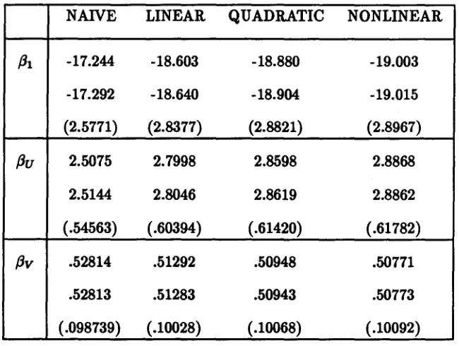
.006078/2).

Table 1 displays results from the SIMEX procedure using NON-lID pseudo errors and the sample

mean as location functional. Four-hundred bootstrap data sets were analyzed. Table entries are,

from top to bottom, point estimates and the means and standard deviations of the 400 bootstrap

sample estimates. For comparison we note that the usual inverse-information standard errors of

the NAIVE estimates are 2.6594, .56436 and .10420 for

fJI,

{Ju and{Jy respectively.

Figure 7b displays estimated response functions for high-risk 50-year old males. The response

functions are graphed over the range

(X.,.,

X.,.+3s)

where

s

is the standard deviation of

{Xi,.H

660_• The two solid curves graph the NAIVE and NONLINEAR SIMEX response curves. The LINEAR

and QUADRATIC SIMEX curves are graphed with dotted and dashed lines respectively. The

. similarity of the SIMEX response functions is due to the small measurement error (0'2 = .003039,

with a linear correction for attenuation = 1.19). For measurement error this small the extrapolant

curves are nearly linear and the three methods of extrapolation produce similar results.

Figure 7c displays graphs ofthe NONLINEAR SIMEX response function (solid line) and selected

bootstrap percentiles enclosing central regions of 90% (dotted), 75% (dashed) and 50% (close dots).

5.9. Exploratory Data Analysis with Mwsured Predictors

Our final example was chosen to emphasize the generaJity and fiexibility of the SIMEX procedure

in deaJing with nonstandard models. Starting with the naive fit of the model (5.1), we considered

the addition of interaction terms of the form X;,~

lti

r2

for small integer powers ({ -1, 0, I}) ofrl

and r2. Taking rl = r2

=

-1 produced the greatest decrease in the deviance, 7.14, although the

improvement in the fit is only marginally significant when compared to a Chi-Squared distribution

with three degrees of freedom (p-value ~ .075). However, the reported p-value is conservative since three is only an approximate degrees of freedom; our model was fit by searching over the

two-dimensional finite set of powers,

(rl' r2),

and the one-dimensional continuous coefficient space.

A model with the measured predictor appearing both on its nominal scale and as an interaction on

an inverse scale provides a nice vehicle for illustrating the fiexibility of the SIMEX procedure.

Therefore we consider fitting the model

pr(Y

=

1

I

U, Y)

=

F

(,81

+

,8uU

+

,8vY

+

,8uv U1

y ) ,

(5.2)

and using the SIMEX procedure to correct for the effects of measurement error.

Table 2 displays coefficient estimates from the SIMEX procedure employing the NON-lID pseudo

errors and the sample mean as location estimator. The inclusion of the interaction term induces

collinearity, making it difficult to interpret individual coefficients. We present instead a graph

similar to that in Figure 7b. Figure 7d displays plots of the NAIVE and NONLINEAR response

curves for two models, with and without the inverse interaction term in (5.2). The response

functions for the models with and without the interaction term are graphed with solid lines and

dotted lines respectively. For both models the SIMEX response function dominates the NAIVE

response function over the range plotted.

6. SUMMARY

We have shown how the results of several coordinated simulation studies,

i.e.,

the{e(~): ~

>

O},

can be used to obtain unbiased or nearly unbiased estimators in nonlinear measurement error models

when the measurement error variance is specified. Our experience suggests that employing

NON-lID pseudo errors and using the sample mean as the location estimator works as well as any other

The success of the method is due in large part to the empirically supported general applicability

ofthe nonlinear extrapolant modela+b/(c+ A). The beauty ofthe method is that the appropriate

values of the parameters a, band c, which for nonlinear models are no longer simple functions of

the data as they are for linear models, are determined by Monte Carlo methods, thereby avoiding

mathematical technicalities and/or resorting to approximations of any type.

It seems likely that the basic method can be improved through the use of more creative

resampling schemes. We are currently exploring the possibility of combining bootstrap resampling

with the Monte Carlo pseudo-error generation in a way that produces both the point estimate and

a standard error without the high computational overhead of nested resampling. Also, it may be

advantageous to use Avalues other than {.5, 1, 1.5, 2}, say by solving an optimal design problem

for the mean modela

+

b/(c

+

A).

Finally we note that the method is applicable to functional as well as structural measurement

error models. This is evident from the results in Sections 4.1, 4.2 and, though not as obviously,

from the resampling simulation in Section 5.1. In the latter case,

Xi,.

remained fixed, as in a

functional model. Thus the method does not depend on the nature (random or fixed) of the

so-called true values

Ui.

This is not true of other methods that explicitly model, either parametrically

or non-parametrically, the

Ui

as random variables.

For example, the regression-calibration method (Prentice, 1982; Fuller, 1987, p 261; Rosneret al.,

1989,1990; Rudemo et al., 1989; GIeser, 1990; Carroll and Stefanski, 1990; and Pierce et al., 1991)

depends on (a model of)

E( U

IX,

V).

The importance of this is that an estimate of

E(U

IX,

V)

obtained from external validation/replication data may not "match" the data to be analyzed in the

sense that the regressions ofUon(X, V)in the validation and target populations need not be equal.

However, methods that depend on external validation/replication data only through estimates of

(72 are generally more robust to differences in the validation and target population distributions.

This is obviously true, for example, when measurement error is due entirely to instrument error

and the error variance is independently assessed via a designed experiment.

REFERENCES

Carroll, R.

J.

& Stefanski, L. A. (1990) Approximate quasilikelihood estimation in models with

•

surrogate predictors. Journal

0/

the American Statistical Association,85, 652--663.

Carroll, R. J. & Stefanski, L. A. (1992) Meta.-Analysis, Measurement Error and Correction for Attenuation. Statistics in Medicine, to appear.

Cook, J. R. (1989) Estimators for the Errors-in-Variables Problem in the Ordered Categorical Regression Model. Unpublished Ph.D. Thesis, Department of Statistics, North Carolina Stae University.

Fuller, W. A. (1984), "Measurement Error Models With Heterogeneous Error Variances," in Topics in Applied Statistics eds. Y. P. Chauby and T. D. Dwivedi, Montreal: Concordia University, pp. 257-289.

Fuller, W. A. (1987). Measurement EfTOr Models. Wiley, New York.

GIeser, L. J. (1990). Improvements of the naive approach to estimation in nonlinear errors-in-variables regression models. In Statistical Analysis

0/

Measurement EfTOr Models and Application,P.J. Brown and W. A. Fuller, editors. AmericanMathematics Society, Providence.

Hwang, J. T. (1986), Multiplicative Errors-In-Variables Models with Applications to the Recent Data Released by U. S. Department of Energy. Journal

0/

the American Statistical Association,

81,680--688.

MacMahon, S., Peto, R., Cutler,

J.,

Collins, R., Sorlie, P., Neaton,

J.,

Abbott, R., Godwin,

J.,

Dyer, A., & Stamler, J. (1990). Blood Pressure, Stroke and Coronary Heart Disease: Part 1, Prolonged Differences in Blood Pressure: Prospective Observational Studies Corrected for the Regression Dilution Bias. Lancet,335, 765-774.

Palca, J. (1990a). Getting to the Heart of the Cholesterol Debate. Science, 24,1170-71.

Palca, J. (1990b). Why Statistics May Understate the Risk of Heart Disease. Science, 24,1171.

Pierce, D. A., Stram, D.O., Vaeth, M., Schafer, D. (1991). Some insights into the errors in variables problem provided by consideration of radiation dose-response analyses for the A-bomo survivors. Preprint.

Prentice, R. L. (1982). Covariate measurement errors and parameter estimation in a failure time regression model. Biometrika, 69, 331-342.

Rosner, B., Willett, W. C. & Spiegelman, D. (1989). Correction of logistic regression relative risk estimates and confidence intervals for systematic within-person measurement error. Statistics in Medicine,8, 1051-1070.

Rosner, B., Spiegelman, D. & Willett, W. C. (1990). Correction of logistic regression relative risk estimates and confidence intervals for measurement error: the case of multiple covariates measured with error. American Journal

0/

Epidemiology, 132, 734-745.

•

with applications to bioassay. Biometrics, 45, 349-362.

Stefanski, L. A. (1985). The effect of measurement error on parameter estimation. Biometrika, 12, 583-592.

Stefanski, L. A. and Carroll, R. J. (1985). Covariate Measurement Error in Logistic Regression.

The Annals of Statistics, 13, 1335-135l.

Stefanski, L.A. and Carroll, R.J. (1981). Conditional Scores and Optimal Scores for Generalized Linear Measurement-Error Models. Biometrika, 14, 103-116.

Whittemore, A. S. and Keller, J. B. (1988). Approximations for Regressions with Covariate Measurement Error. Joumal of the American Statistical Association, 83, 1051-1066.

•

•

•

TABLE 1: COMPARISON OF ESTIMATORS. This simulation is described in Section 5.2. Table entries are from top to bottom, point estimates, bootstrap means and bootstrap standard

errors. Inverse information standard errors for the NAIVE estimates are 2.6594, .56436 and .10420 for

f3t, f3u

and

f3v

respectively.

NAIVE LINEAR QUADRATIC NONLINEAR

f31

-17.244 -18.603 -18.880 -19.003

-17.292 -18.640 -18.904 -19.015

(2.5771) (2.8377) (2.8821) (2.8967)

f3u

2.5075 2.7998 2.8598 2.8868

2.5144 2.8046 2.8619 2.8862

(.54563) (.60394) (.61420) (.61782)

f3v

.52814 .51292 .50948 .50771

.52813 .51283 .50943 .50773

(.098739) (.10028) (.10068) (.10092)

TABLE 2: COMPARISON OF ESTIMATORS. NAIVE and SIMEX estimates for the model with inverse interaction (5.2).

NAIVE LINEAR QUADRATIC NONLINEAR

f31

6.1604 5.1932 4.9685 4.8446

f3u

1.0654 1.3413 1.3974 1.4222

f3v

-1.1709 -1.2191 -1.2260 -1.2278