Copyright 0 1992 by the Genetics Society of America
Persistence of Repeated Sequences That Evolve
by
Replication Slippage
Hidenori Tachida* and Masaru Iizukat
*National Institute of Genetics, Mishima, Shituoka-ken 4 1 1, Japan, and ?General Education Course, Chikushi Jogakuen Junior College, Dazaijk-shi, Fukuoku-ken 818-01, Japan
Manuscript received September 24, 1991 Accepted for publication February 8, 1992
ABSTRACT
T h e evolution of short repeated sequences by replication slippage under the assumption of selective neutrality is modeled using a linear birth and death process. T h e equilibrium distribution, the distribution of the life expectancy of a repeated sequence when the process starts from two repeats,
the age distribution of repeats, the probability of obtaining two genes with i and j copies which diverged t generations ago and the conditional variance of copy number given the repeat number is more than one are computed. The distributions of life expectancy and age are shown to have long tails. Also the statistic which estimates the conditional variance is shown to have a large coefficient of variation. Using these theoretical results, we develop an approximate test of our model and analyze
persistent repeated sequences found in the primate @-globin gene region and Oenothera chloroplast
DNA which are polymorphic within species. We found one sequence in Oenothera chloroplast DNA
which does not fit to our neutral model.
A
wide variety of simple repetitive sequences occurfrequently in eukaryotes (BLAISDELL 1983;
TAUTZ, TRICK and DOVER 1986). T h e copy number
of those repeated sequences is known to vary (JONES
and KAFATOS 1982; MOORE 1983). For short repeated sequences, replication slippage (slipped-strand mis-
pairing) rather than unequal crossing over is consid-
ered to be a major factor influencing copy numbers
(TAUTZ, TRICK and DOVER 1986; LEVINSON and GUT-
MAN 1987).
In contrast with unequal crossing over between homologous chromosomes as analyzed by OHTA and KIMURA (1 98 l ) , TAKAHATA (1981) and STEPHAN (1986, 1987), replication slippage is a process which does not involve the homologous chromosome. Thus,
it is considered to be a specific type of mutation
process and can be treated similarly as the stepwise
mutation model of OHTA and KIMURA (1 973). WALSH
(1 987) considered a population genetic model which incorporates replication slippage as an evolutionary force. He computed the equilibrium distribution and
the expected mean persistence time of repeats in terms
of slippage events assuming either no selection or
selection that imposes a lower bound on the number of repeats.
Here, we model the evolution of short repeated sequences by replication slippage using a linear birth
and death process to extend the work of WALSH
(1 987) assuming selective neutrality (KIMURA 1983,
199 1) with regard to repeat number. We compute the
equilibrium distribution, the distribution of the per- sistence time in terms of generations, the age distri-
bution of repeats and the probability of obtaining two
Genetics 131: 471-478 (June, 1992)
genes which diverged t generations ago and contain i
and j repeats, respectively. Using these theoretical
results, we analyze the persistent repeated sequences found in the flanking region of primate B-globin genes
(SAVATIER et al., 1985) and in the chloroplast DNA
of Oenothera (WOLFSON, HICGINS and SEARS 1991).
One sequence was found to be inconsistent with our neutral model.
MODEL
Replication slippage is a mechanism by which the number of short, tandemly repeated sequences in- creases or decreases when DNA is replicated [see
LEVINSON and GUTMAN (1987) for details]. Let i be
the number of repeats in a repeated sequence. We
call the region containing the DNA sequence a gene
and ignore recombination therein. We do not know
the exact shape of the function which relates the number of repeats to the rate of slippage at present. However, if the number of repeats increases, the rate of slippage is thought to increase because the proba- bility of mispairing increases. This was shown to be the case when bacteriophage T 4 DNA was used
(STREISINGER and OWEN 1985). Here, for simplicity,
we assume that only one repeat is added or lost per
generation and denote these rates by
(i
-
l)ul and(i
-
l)uq, respectively, when the number of repeats isi(i 2
2).
WALSH (1987) assumed rates of iul and iu2,respectively, but this makes little difference at equilib- rium as we show later. We denote the rate of increase
from one repeat to two repeats by ‘u since the mecha-
nism of increase is different from the other cases. We
= uz/ul is less than or equal to one, WALSH (1987) showed that the equilibrium distribution does not exist. This is because the number of repeats increases to infinity with a positive probability. We do not
observe a very large number of repeats except in
specific regions of DNA such as satellite DNA. Also
data from phage T 4 indicates that the rate of deletion
is always larger than the rate of addition (STREISINGER
and OWEN 1985). Thus, we assume that T is larger
than one in the following. Furthermore, we assume that the number of repeats does not affect the fitness of the carrier.
First, we consider the equilibrium distribution, p , ( i ) ,
of the number of repeats. Let p(i,t) be the probability
that the number of repeats is i at generation t. Consid-
ering respective events which occur in one generation,
the transition equations for p(i,t) are
p ( l J
+
1) = (1-
v ) p ( l , t )+
U2P(2,t)p(2,t
+
1) = [ I-
(u1+
ue)]p(P,t)i- vp(1,t)
+
2@2p(3,t)(1) p(i,t
+
1) = [ l-
(2-
l ) ( U l+
up)]p(i,t)+
(i-
2)u1p(i-
1,t)+ iupf(2 +
1J). ( i 3 3).When u1, up, v are small compared to one, the p(i,t)'s
approximately satisfy the differential equations,
-
d dt ( 1 4 = -vp( 1 ,t)+
Uzp(2,t)+
(i-
2)u1p(i-
1,t)+
iupp(i+ 1,t).
(i 2 3).Letf(z,t) be the generating function of p(i,t) defined as
m
f(z,t) =
2
P ( i , t ) P . (3)i= 1
From the above differential equations, we can show
that the generating function f(z,t) satisfies a partial
differential equation
"
af(zJ) u,(z
-
r)(z-
1)-
af(zJ)-
-
v(z-
l) P (l ,t) (4)at
a zwhere r = u2/uI. Letf,(z) be the equilibrium solution
of this equation. Then,f,(z) satisfies
-u,(z
-
r)(z-
1)df,o
= v(z-
I)P*(l). (5)dz
T h e solution which satisfiesf,( 1) =
cE1
p , ( i ) = 1 isUsing the relationshipf,(O) = p*(l), we can soIve for
P * ( l ) ,
By expanding the right hand side of (6) and matching coefficients, we obtain the equilibrium distribution for i 3 2,
Next we consider the dynamics of the number of repeats in one lineage. Since we expect v
<<
u1, up, weignore v and investigate the time dependent behavior
of the number of repeats starting from io repeats at
generation 0. We usually suppress io in the expression
for ease of presentation when the initial condition is
obvious from the context. Then (2) with v = 0 is
approximated by a differential equation
d p W ) dt
"
-
-(i-
l)(Ul+
Up)p(i,t)+
(i-
2)u1p(i-
1 ,t)+
iupP(i+
1,t).where p(0,t) = 0. Since this is a differential equation
for a linear birth and death process, we can solve this
by a standard method (Cox and MILLER 1965; IIZUKA
1989). T h e generating functionf(z,t) satisfies
a f w
-
u,(z-
r)(z-
1)a f o
= 0. (10)at
m
T h e solution which satisfies the initial condition
f(z,O) = z'0-l is
(exp(st)
-
r)z-
r(exp(st)-
1) (exp(st)-
l ) z-
( r exp(st)-
1)where s = ul(r
-
1). By expanding the right-hand sidewith regard to z and matching coefficients, we obtain
p(i,t),
p(1,t) = a'o-l (1 2)
(i- l)A(io- 1)
p(i,t) =
k= 1 2 - 1 - k
.
ato-k-lpkyi-l-k (i>
1)where
r(exp(st)
-
1) ( r-
l)'exp(st)r exp(st)
-
I = ( r exp(st)-
1)' (14)exp(st)
-
1r exp(st)
-
1 *a =
Replication slippage 473
2 . 0 1
-,= 1.1
- - r = 1 . 3
- - -r=1.5
r = 2.0 .""
0 0 . 5 1 1 . 5 2 2 . 5 3 3 . 5 4
u,t
FIGURE 1 .-Density of life expectancy as a function of ult. Life
expectancy is the time required for the number of repeats to become
one starting from two repeats.
i A j denotes the smaller of the numbers i, j . In the
special case of io = 2, the solution has a simple form
p(1,t) = ff (15) p ( i , t ) = pyi-2. (i
>
1) (16) By examining p(l,t), we can investigate the timerequired for the repeated sequences to become a
single copy sequence. Let T be the time when the
number of repeats becomes one starting from two
repeats. T is considered to be the life expectancy of
the repeated sequence. Then
Prob[T S t ] =
p (
1 ,t). (17)
T h e density of T is obtained by taking a derivative of
this function. We computed the density of the life
expectancy as a function of scaled time ult as
( r
-
1)*r exp[(r-
l)ult]( r exp[(r
-
l)ult]-
( 1 8)and plotted it for several values of r in Figure 1. T h e density function is always monotone decreasing. Also
the life expectancy is longer for smaller r since r =
u2/u1 and the deletion rate is smaller in this case.
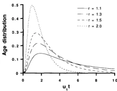
Another quantity of interest is the age distribution
of the repeat when we sample a gene which has i
repeats. Since a new repeated sequence is created at
a constant rate v and since the number of repeats is
initially two, the age distribution, q ( i , t ) , becomes
at equilibrium. T h e age distribution of a gene which now has six repeats is plotted as a function of ult for
various values of r in Figure 2. Although the peaks of
the distributions are located near ult = 2, the tail of
the distribution is very long, especially for small r.
-r = 1.1
- - r = 1.3
- - - r = 1.5
r = 2.0
" ~ ~ .
0 2 4 6 8 1 0
"1
FIGURE 2.-Age distribution of a repeated sequence as a function of u l t . The age distribution of a repeated sequence which now has
six repeats is plotted for various values of r .
Thus, if r is small, the origin of the repeats could be
very old.
Finally, we consider the evolution of two genes which have a common ancestor at time zero. We are
interested in the probability,
p(i,j,t),
that the numberof repeats,
I
and J , in the two genes which have acommon ancestor t generations ago are
i
and j , re-spectively. As an approximation, we again assume that
v is so small that creation of a new repeated sequence
occurs at most once during the time we consider.
Then, if we observe more than one repeat in both
genes, the repeated sequences are not created after the common ancestor and the common ancestor gene should have two or more repeats. Thus, we can ignore
v in the evolution of these two genes when we consider
p ( i , j , t ) (i
2,
j 3 2) and the transition equation forp ( i , j , t ) is
p ( i , j , t
+
1) = [ l-
(i+
j-
2)](u1+
up)p(i,j,t)+
(i-
2)UlP(i-
I&)+
( j-
2)Ul@(i,j-
1,t)+
iu,p(i+
1,jJ) +ju$(i,j+
1,t). (20)Here, we assumed that u1 and u2 are small so that at
most one event of change occurs in the two genes in the same generation. With the initial condition
p(i,j,o)
=p * ( i )
(i =j )
= o
(i f j ) ,p ( i , j , t ) is computed to be [see (A6) in the APPENDIX]
where
6. . = ( I
-
l)!(-l)a+j-'( I
-
i+
l)!(I-
j+
l)!(i+
j
-
I-
2)!*i V j denotes the larger of the numbers i, j .
defined as
One summary measure is the conditional variance
-
-
Prob[I k 2, J k 21
T h e expectation which appears in the numerator of the right-hand side is taken over the event ( I k
2,
Ja
2). From ( A 1 3) in the APPENDIX,E [ v I Z b 2 , J k 2
1
(23) \ I - e - 2 s y 1
-
(?-'sf)-
-
( r
-
1 )'Iog(l-
e-2st/r)'T h e left-hand side converges to r / ( r
-
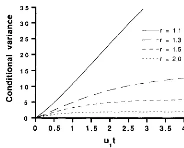
1)' as t ap- proaches infinity. Numerical values of the conditionalvariance as a function of ult are shown for various
values of r in Figure 3. For large r ( r = 2.0), the conditional variance is very small. This is because we
observe I = 2, J = 2 in most of the cases when r is
large. For r = 1 . 1 , the conditional variance increases
linearly until about ult = 5. It then starts to level off
and attains the final value, 110, at about ult = 20
(data not shown). For smaller values of r , the approach
to the final value is quicker.
In a similar way, we can compute the variance,
Var[(Z -J)'/'
I
I 2 2, J k 21 of the conditional variance. It is expressed as-( 1
-
e-2sf)(~(r,st)e2sfIog(l-
e-2st/r)+
(1-
e-'s1)) (r-
1)4e4s'[Iog( 1-
e-2sf/r)12 (24)where
{(r,st) = (r'
+
10r+
1)-
6(2r+
l)e-"l+
6e-4st.As st becomes large, the variance approaches ( r 3
+
9r'
+
r ) / ( r-
1)". T h e coefficient of variation of ( I-
J)'/2 approaches [(r'+
9r+
l)/r]'/' which isabout 3.3 for 1
s
rc
2. Thus the coefficient ofvariation (the ratio of the standard deviation to the mean) for this statistic is very large.
T h e above formula is for genes whose common
ancestor existed t generations ago. Thus, it can be
applied to two genes, each taken from different spe- cies, whose divergence time is known. Often two genes
are sampled from the same species, so we now consider
this case. T h e time until a common ancestor is a
random variable determined by the population struc-
ture. Assume that the population size has been a
constant N and that the population is mating ran-
domly. Let T be the time until the common ancestor.
Then, the distribution of T is exponential [see for
0 0.5 1 1 . 5 2 2 . 5 3 3.5 4
"1
FIGURE 3.-The conditional variance given that two genes both
have more than one repeat when the two genes have a common ancestor t generations ago.
example, TAJIMA (1 983)]
Prob[T 6 t] = 1
-
exp(-t/2N). ( 2 5 )Using this distribution, we can compute the denomi-
nator and the numerator of Equation 22. T h e denom-
inator is calculated using the Taylor expansion of the logarithm function:
Prob[Z 3 2, J k 21
m
2N
= c .
I = ] z(1+
4Nsi)r"T h e numerator of Equation 22 is
E[?, ( I 3 2, J 3
2)
I
4NvP*(l)s
-
-
U I ( T
-
1)'(1+
4 N ~ ) ( l+
8Ns)'Combining (26) and
(27),
we obtain the conditionalvariance when genes are taken from a population,
4Ns
-
-
m1
( r
-
1)'(1+
4Ns)(l+
8Ns)2
. 1z(1
+
4Nsi)r'We can compute the denominator numerically by
truncating the sum since all the terms are positive.
Unless T is very close to one, the convergence is fairly
quick. T h e conditional variance as a function of 4Nul
is shown for various values of r in Figure 4. Even for
large 4Nul, the conditional variance is small for r k
Replication slippage 475
0
r = 1.05
."" r = 1.5
r = 2 0 " . . .
"-- """""""
0 1 2 3 4 5
4Nu,
FIGURE 4.-The conditional variance given that two genes both
have more than one repeat when the two genes are taken from a population of size N.
give much information on 4Nul when 4Nul is more
than one. For smaller values of r , the conditional
variance increases as 4Nul increases, but it converges to a constant when 4Nu1 becomes very large (data not shown).
STATISTICAL TEST
When data on variation within and between species is available, we can test the model by examining
whether the two types of data can be explained by the
same parameter set or not. If we can not find such a
parameter set, we reject the null hypothesis that the model is correct. Here, we develop an approximate
test for our model which examines whether the vari-
ation between species is smaller than that expected from the variation within species. In other words, this
test examines whether some force such as selection
should be invoked when we find a persistent repeated sequence.
Let
Z
and J be the numbers of repeats in a pair ofgenes which have a common ancestor t generations
ago (Figure 5). Let K and L be numbers of repeats in
another pair of genes which have a common ancestor
ct generations ago. In the present context,
Z
and Jcome from the same species and K and L come from
different species. Define a probability Q(i,k,m,n,ul,
t,r,c) as
This is a probability that if we sample two pairs of genes, the first pair have different number of repeats
(difference is more than m) and the second pair have
similar numbers (difference is less than or equal n) of
repeats. If two pairs of genes are independent, the right-hand side of the equation becomes
Prob[(Z
-11
>
mlZ =21
X Prob[IK
-
LIc
n l K =k].
. ,
t c & J L
I J K L
FIGURE 5.-The relationships of gene pairs. The two genes
which have I and] repeats, respectively, have a common ancestor t
generations ago. The two genes which have K and L repeats, respectively, have a common ancestor ct generations ago.
These two terms can be computed using Equations 21 and 8,
Prob[lZ
-
J I
>
mlZ =i]
i+m
Prob[lK
-
LI d n l K =k]
k+n
Note that these are functions of only
i, k,
m, n, ult, r,c and do not depend on v . Thus, we write the proba-
bility in (29) as Q(i,k,m,n,ult,r,c) from now on. We
search over a set of parameters u l t , r which give rise
to Q larger than K (significance level) for a given set
of data
i,
k,
m, n. T h e factor c is estimated by usingother data such as sequence differences. If we can not
find such a parameter set, we reject the null hypothesis
that the repeated sequences are evolving neutrally
with the same parameter set u1 and r. Because we
search a set of parameters ult, r , this test is conserva- tive.
We apply this test to persistent repeated sequences
found in the 5' flanking region of the primate
p-
globin genes (SAVATIER et al. 1985) and in the chlo-
roplast DNA of Oenothera (WOLFSON, HIGCINS and
SEARS 199 1).
SAVATIER et al. (1985) sequenced a 5500 base-pair
fragment including the 5' flanking region of the
p-
globin gene in chimpanzee. Comparing this sequence
with the corresponding sequence in human (PONCZ et
al. 1983), they found four repeated sequences (RSI-
RS4) whose repeat numbers vary between the two
species. Three of them (RS1-RS3) are also found in
macaque (SAVATIER et al. 1987a). Also for some se-
quences, data on variation within human populations
is available. Repeat numbers of those repeated se-
quences are summarized in Table 1. Among the four
sequences, we applied our test to RS2 and RS3 since
they are found in macaque and also because data on variation within species are available for them. T h e
TABLE 1
Number of repeats of tandem repeated sequences found in the
5' flanking region of primate @-globin genes
Repeat Chimp." Mac.b H u m l C Hum2" Hum3" Sequence
RS 1 8 45 7 (TG)"
RS2 10 12 16 17 (TG)-
RS3 3 5 6 5 7 (ATTTT),
RS4 12 None 7 11 8 (AT),
Numbers of repeats in chimpanzee (Chimp.), macaque (Mac.) and human (Huml-3) are shown. Blanks in the table indicate missing data. Multiple samples are taken from human populations. Hum2 and Hum3 denote different individuals from different re- peated sequences. Naming of the repeated sequences (RSl-RS4) is from SAVATIER et al. (1987b).
"
From SAVATIER et al. (1 985). From SAVATIER et al. (1 987a).From PONCZ et al. (1 983).
flanking region of the human ,&globin gene is 0.0035
(computed from the data of the 1-kb region in
CHEBLOUNE et ul. 1988). T h e corrected proportion of
differences in the corresponding region between hu-
man and macaque is 0.046 (IG4 and IG5 of SAVATIER
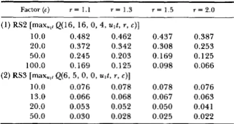
et ul. 1987b). Thus, the factor c is estimated to be 13. We randomly assigned Huml-Hum3 of RS3 or
Huml-2 of RS2 to 1, J , K in Figure 5 and computed
mu~~,~Q(i,ll,m,72,u~t,~,c) for various values of c and r
using data of RS2 and RS3. T h e data of RS2 is well
explained by our model even if we assume c to be
more than 100. However the probabilities for the data
of RS3 are close to 0.05 as shown in Table 2. Consid-
ering that our test is conservative, we suspect that
some force might be operating to lengthen the per- sistence of the repeated sequence.
WOLFSON, HIGGINS and SEARS (1991) sequenced a
region of Oenothera chloroplast DNA from four plas- tomes. Plastomes are types of chloroplast found in
related species of Oenothera. They found two
stretches of adenosine residues whose sizes change
among plastomes in noncoding regions. T h e data are
summarized in Table 3 with those from Nicotiana.
We estimated c to be 39 using the divergence of
nucleotides in the coding region among those chlo-
roplasts shown in Figures 2 and 3 of WOLFSON, HIG-
GINS and SEARS (1 99 1). We randomly assigned plas- tomes 11, IV and 111 to I , J and K (see Figure 5 ) and
computed mux,ltf2(i,k,m,n,ult,r,c). T h e sequence of
Nicotiana is assigned to be L. Though repeat I is well
explained by our model even with a c value of more
than 100 (data not shown), the maximum probability is very small for repeat 11 as shown in Table 4. Even
when c is seven, the maximum probability is less
than 0.05. Thus, we reject the null hypothesis for repeat 11.
DISCUSSION
In our model, we assumed that the rate of replica-
tion slippage is proportional to one less than the
TABLE 2
The maxima of Q(i, k, m, n, u ~ t , r, c) for the repeated sequences
in 5' region of primate @-globin genes
Factor(c) r = 1 . 1 r = 1 . 3 r = 1.5 r = 2 . 0
(1) RS2 [max,,, Q(16, 16, 0, 4, u l t , r , c)]
10.0 0.482 0.462 0.437 0.387
20.0 0.372 0.342 0.308 0.253
50.0 0.245 0.203 0.169 0.125
100.0 0.169 0.125 0.098 0.066
(2) RS3 [max,,, Q(6, 5, 0, 0, w t , r , c)]
10.0 0.076 0.078 0.078 0.076
13.0 0.066 0.068 0.067 0.063
20.0 0.053 0.052 0.050 0.041
50.0 0.030 0.028 0.025 0.022
For definitions of r , c, and Q(i, k , m, n, u i t , r , c), see the text.
TABLE 3
Number of repeats in the repeated sequences found in the
chloroplast DNA of four Oenothera plastomes and Nicotiana
tabacum
Plastome
Repeat Nicotiana I 11 I11 IV Sequence
I 8 13 13 14 14 (A),
I1 9 I 1 12 19 19 (A).
Made from WOLFSON, HICCINS and SEARS (1991). Naming of the repeated sequences (I, 11) is arbitrary determined.
TABLE 4
The maxima of Q(12, 19, 6, 10, u,t, r, c) for repeat I1 in
chloroplast DNA of Nicotiana and Oenothera
Factor(<) r = l . l r = 1 . 3 r = 1 . 5 r = 2 . 0
7.0 0.043 0.012 0.005 0.001
10.0 0.028 0.006 0.002 0.000
20.0 0.010 0.001 0.000 0.000
50.0 0.002 0.000 0.000 0.000
For definitions of r , c, and Q(i, k, m, n , ult, r , c), see the text.
number of repeats. We used this linear function be-
cause it is increasing and also it makes the calculation
easier. There is not much information on the shape
of this function at present. STREISINGER and OWEN
(1985) observed that the rate of insertion or deletion increased 100-fold when the number of repeats was increased from four to five in T 4 DNA. However, if such a rapid increase of the slippage rate occurs, we would not observe repeat numbers of several or more in DNA sequences. Indeed, using Equations 8a and
8b of WALSH (1 987), we obtain
P * ( i )
-
&+Ip , ( i
+
1)x,
(33)Replication slippage 477
respectively, of the repeat number when the number of repeats is
i.
If p5 is a hundred-fold of X 4 as in theirdata, we would observe p5/p4
<
1/100 and this is notthe case (see Table 1). Therefore, we think that the rate increases less rapidly than the rate of T 4 DNA in STREISINGER and OWEN (1 985) as the repeat number
increases. WALSH (1 987) used another linear function
which is proportional to the number of repeats. Under
his model, the ratio of p , ( i ) to p * ( i
+
1) iswhereas in our model it is
P J i )
-
irp * ( i
+
1) i-
1’(34)
(35)
We can see that there is not much difference in the equilibrium distribution, especially for a larger num- ber of repeats as long as we use a linear function for the slippage rate. Therefore, the conclusion as to the neutrality of the persistent repeated sequences ana- lyzed above will not be changed if the shape of the function is linear.
We found one repeated sequence (repeat 11) in the Oenothera chloroplast which is inconsistent with our
model and another (RS3) in the &globin gene region
which is suspected to reject our model. In both cases, the changes in the number of repeats are too small
when we compare the repeat numbers between differ-
ent species. Although there are uncertainties about
the estimation of c, our model is rejected even if we
assume c to be seven for repeat I1 of Oenothera
chloroplast. Since our test is conservative, the se-
quence seems to be evolving differently from our
model. Also the power of our test is low since it utilizes only a few sequences. If we can devise tests which
utilize more sequences, the data on RS3 may become
significant.
We mention three possibilities for what caused re-
jection of our model in repeat I1 and possibly in RS3.
One is that selection keeps the repeat number in a
certain range. In this case, the repeated sequence has
a biological function. It is noteworthy that another
repeated sequence, RS4, in the primate P-globin re-
gion can bind some erythroid-specific factor modulat-
ing @-globin gene expression (BERG et aE. 1989). A
second possibility is that ui may change in the lineages
of two species. If the ui’s are larger in the species in which data on the variation within species is available,
we obtain such a pattern. A third possibility is the
inadequacy of our slippage model. For example, if the
repeat number changes more than one per genera- tion, we may obtain a pattern like that in repeat I1 of Oenothera without selection. In addition to more data, further theoretical studies are necessary to in- vestigate these possibilities.
We thank V. M. NIGON for introducing this problem to us and C. BASTEN, C. GAUTIER, M. GOUY, V. M. NIGON, P. PERRIN- PECONTAL, B. WALSH and an anonymous reviewer for comments on the manuscript. This research was partially supported by NIG Cooperative Research Program (’91-35) and a grant-in-aid from the Ministry of Education, Science and Culture of Japan. This is contribution no. 1900 from the National Institute of Genetics, Mishima, Japan.
LITERATURE CITED
BERG, P. E., D. M. WILLIAMS, R. B. COHEN, S. CAO, M. MITTELMAN
and A. N. SCHECHTER, 1989 A common protein binds to two silencers 5’ to the human @-globin gene. Nucleic Acids Res.
17: 8835-8852.
BLAISDELL, B. E., 1983 A prevalent persistent global nonrandom- ness that distinguishes coding and non-coding eukaryotic nu- clear DNA sequences. J. Mol. Evol. 1 9 122-133.
CHEBLOUNE, Y., J. PAGNIER, G. TRABUCHET, C . FAURE, G. VERDIER, D. LABIE and V. M. NIGON, 1988 Structural analysis of the
5’ flanking region of the beta-globin gene in African sickle cell anemia patients: Further evidence for a triple origin of sickle mutation in Africa. Proc. Natl. Acad. Sci. USA 85: 4431-4435.
Cox, D. R., and H. D. MILLER, 1965 The Theory of Stochastic Processes. Chapman & Hall, London.
IIZUKA, M., 1989 A population genetical model for sequence evolution under multiple types of mutation. Genet. Res. 5 4
231-237.
JONES, C. W., and F. C . KAFATOS, 1982 Accepted mutations in a gene family: evolutionary diversification of duplicated DNA. J.
KIMURA, M., 1983 The Neutral Theory of Molecular Evolution.
Cambridge University Press, Cambridge.
KIMURA, M., 1991 Recent development of the neutral theory viewed from the Wrightian tradition of theoretical population genetics. Proc. Natl. Acad. Sci. USA 88: 5969-5973.
LEVINSON, G., and G . A. GUTMAN, 1987 Slipped-strand mispair- ing: a major mechanism for DNA sequence evolution. Mol. Biol. Evol. 4: 203-221.
MOORE, G. P., 1983 Slipped-strand mispairing and the evolution of introns. Trends Biochem. Sci. 8: 41 1-414.
NEI, M., and F. TAJIMA, 1981 DNA polymorphism detectable by restriction endonucleases. Genetics 97: 145-163.
OHTA, T., and M. KIMURA, 1973 A model of mutation appropri- ate to estimate the number of electrophoretically detectable alleles in a finite population. Genet. Res. 22: 201-204.
OHTA, T., and M. KIMURA, 198 1 Some calculations on the amount of selfish DNA. Proc. Natl. Acad. Sci. USA 78: 1129-1 132.
PONCZ, M., E. SCHWARTZ, M. BALLANTINE and S. SURREY,
1983 Nucleotide sequence analysis of the delta-beta globin
gene region in human. J. Biol. Chem. 2 5 9 11599-1 1609.
SAVATIER, P., G. TRABUCHET, C. FAURE, Y. CHEBLOUNE, M. GOUY, G. VERDIER and V. M. NIGON, 1985 Evolution of the primate beta-globin gene region: High rate of variation in CpG dinu- cleotides and in short repeated sequences between man and chimpanzee. J. Mol. Biol. 181: 21-29.
SAVATIER, P., G. TRABUCHET, Y. CHEBLOUNE, C. FAURE, G. VER-
DIER and V. M. NIGON, 1987a Nucleotide sequence of the
beta-globin genes in gorilla and Macaque: The origin of nu- cleotide polymorphisms in human. J. Mol. Evol. 24: 309-3 18.
SAVATIER, P., G. TRABUCHET, Y. CHEBLOUNE, C. FAURE, G. VER-
DIER and V. M. NIGON, 198713 Nucleotide sequence of the
delta-beta-globin intergenic segment in the macaque: structure and evolutionary rates in higher primates. J. Mol. Evol. 2 4
STEPHAN, W., 1986 Recombination and the evolution of satellite Mol. EvoI. 19: 87-103.
297-308.
STEPHAN, W., 1987 Quantitative variation and chromosomal lo-
cation of satellite DNAs. Genet. Res. 5 0 41-52.
STREISINGER, G., and J. OWEN, 1985 Mechanisms of spontaneous
and induced frameshift mutation in bacteriophage T4. Ge-
netics 109 633-659.
TAKAHATA, N., 1981 Mathematical study of distribution of the
number of repeated genes per chromosomes. Genet. Res. 38:
TAJIMA, F., 1983 Evolutionary relationship of DNA sequences in
finite populations. Genetics 105: 437-460.
TAUTZ, D., M. TRICK and G. A. DOVER, 1986 Cryptic simplicity
in DNA is a major source of genetic variation. Nature 3 2 2
WOLFSON, R., K. G. HIGGINS and B. B. SEARS, 1991 Evidence for
replication slippage in the evolution of Oenothera chloroplast
DNA. Mol. Biol. Evol. 8: 709-720.
WALSH, J. B., 1987 Persistence of tandem arrays: implications for
satellite and simple-sequence DNAs. Genetics 115: 553-567.
97-102.
652-656.
Communicating editor: E. THOMPSON
APPENDIX
Computation of p ( i J , t ) : Let f(x,y,t) be the gener- ating function of p ( i , j , t ) defined as
m m
f(x,y,t)
= p ( i , j , t ) x i - l y - l . (AI)i=l j = 1
If we use the continuous time approximation as in the
one gene case, we can derive a partial differential
equation satisfied by f(x,y,t) using (20),
9-
u,(x-
r)(x-
1) dfat
-
u1(y-
r)(y-
1)-
df
= 0.ay
If we take two genes randomly, the common ancestor is again a random sample. Thus, if we assume that the population is in the equilibrium state at generation
zero, the distribution of the repeat number in the
common ancestor gene is p,(i). Therefore, the initial
condition for p ( i j , t ) is
P ( i j , O ) f P*(i) (i = j )
= o
(iZj).
From these, the initial condition for
f(x,y,t)
is com-puted to be
m
f(x,y,O) = p*(i)X'"y"l
= f*(XY)
I= 1 (A4)
wheref, is the generating function of the one gene case in the equilibrium state [see eq (S)]. T h e solution of (A2) which satisfies this initial condition is
( r
-
x)(r
-
y)eZsf-
r( I-
x)(l-
y) [(resf-
1)-
(esf-
1) x][(re"
-
1)-
(esf-
l)y]We can compute p ( i , j , t ) by expandingf(x,y,t) with
respect to x and y and matching coefficients. T h e
resulting expression for
i
b2
and j 5 2 is[I
-
exp(-2st)]2"i-J+2[1-
exp(-2st)l'+j-i-2 ri+j-'-'[r-
exp(-2st)l'where
( a
-
1)!(-1)+-l 6 . . =I J . ~
( 1
-
i
+
1)!(1-
j+
I)!(i+
j-
I
-
2)!* Conditional variance: First we compute the de- nominator of (22) which can be expressed asProb[Z 3 2, J 3 21 = 1
-
Prob[Z = 11('47)
-
Prob[J = 13+
Prob[Z = 1, J = 11. Noting the following relationshipsf(x,y,t)lx=O,y=l
= Prob[Z = 11 (AS)f(x,y,t)lx=O,y=O
= Prob[Z = 1, J = 13 (A9) and using (A5),Prob[Z 5 2, J 2 21 =
--
vp*(l)log( 1-
7).
(A10)U1
Next we compute the numerator of (22). First, note that the variance is represented by
E [ u , (Z 3 2, J 3 211 2
m m
=
C,
(2'-
29+
j2)p(i,j,t)/2.i=2 j-2
Using derivatives of f(x,y,t), we can compute the right-
hand side and we obtain
-
vp,(l)(e"'-
l)(esf+ 1)
-
u l ( r
-
1)ze4srFrom equations (A1 0) and (A1 2), the conditional var-
iance is computed to be