Deleterious mutations, apparent stabilizing selection and the maintenance of quantitative variation.

(1)

Copyright 0 1992 by the Genetics Society of America

Deleterious Mutations, Apparent Stabilizing Selection and the Maintenance

of Quantitative Variation

**Alexey S. Kondrashov*9’ and Michael**

Turellit

*Institute of Mathematical Problems of Biology, Pushchino, Moscow Region 142292, Russia, and TDepartment of Genetics and Center for Population Biology, University of Calijornia, Davis, Calijornia 95616

Manuscript received December 3, 199 1 Accepted for publication June 30, 1992

ABSTRACT

Apparent stabilizing selection on a quantitative trait that is not causally connected to fitness can result from the pleiotropic effects of unconditionally deleterious mutations, because as N. Barton noted,

“. . . individuals with extreme values of the trait will tend to carry more deleterious alleles

. . . .”

We use a simple model to investigate the dependence of this apparent selection on the genomic deleterious mutation rate, U ; the equilibrium distribution of K , the number of deleterious mutations per genome; and the parameters describing directional selection against deleterious mutations. Unlike previous analyses, we allow for epistatic selection against deleterious alleles. For various selection functions and realistic parameter values, the distribution of K , the distribution of breeding values for a pleiotropically affected trait, and the apparent stabilizing selection function are all nearly Gaussian. The additive genetic variance for the quantitative trait is kQa‘, where k is the average number of deleterious mutations per genome, Q is the proportion of deleterious mutations that affect the trait, and a 2 is the variance of pleiotropic effects for individual mutations that do affect the trait. In contrast, when the trait is measured in units of its additive standard deviation, the apparent fitness function is essentially independent of Q and a‘; and

8,

the intensity of selection, measured as the ratio of additive genetic variance to the “variance” of the fitness curve, is very close to s = U / k , the selection coefficient against individual deleterious mutations at equilibrium. Therefore, this model predicts appreciable apparent stabilizing selection if s exceeds about 0.03, which is consistent with various data. However, the model also predicts that must equal VJV,, the ratio of new additive variance for the trait introduced each generation by mutation to the standing additive variance. Most, although not all, estimates of this ratio imply apparent stabilizing selection weaker than generally observed. A qualitative argument suggests that even when direct selection is responsible for most of the selection observed on a character, it may be essentially irrelevant to the maintenance of variation for the character by mutation-selection balance. Simple experiments can indicate the fraction of observed stabilizing selection attributable to the pleiotropic effects of deleterious mutations.

-

T

WO alternative theories of mutation-selection balance have coexisted peacefully for the last 60 years. T h e first is the classical theory of equilibrium between mutation to unconditionally deleterious alleles and directional selection against them. HALDANE

(1 927) considered completely recessive mutations;

WRIGHT (1929), EFROIMSON (1932) and HALDANE

(1937) treated one locus with some degree of domi- nance. T h e multilocus case was studied first by KI-

MURA and MARUYAMA (1 966) (see also CROW 1970), and its behavior and implications were elaborated by

KONDRASHOV (1982, 1984, 1988) and CHARLES-

WORTH (1990). These models assume that fitness decreases with the number of deleterious alleles carried, and they do not relate fitness directly to selection on specific phenotypes. For realistic parameter values, only one mutation-selection equilibrium is possible,

ison, Wisconsin 53706.

Genetics 132: 603-618 (October, 1992)

’

Present address: Laboratory of Genetics, University of Wisconsin, Mad-

with the “wild-type” alleles in high frequency at all loci [multiple equilibria appear only when deleterious alleles are completely recessive (ALLENDORF 1979)].

The second theory, concerned with maintaining genetic variance for quantitative traits, was introduced

by FISHER (1930, Ch. 5) and WRIGHT (1935) and

developed by LATTER (1960) and LANDE (1975, 1980). Inspired by LANDE’S (1975) observation that its parameters may be estimated from quantitative genetic experiments, this theory has enjoyed much more attention in recent years [reviewed by BULMER

(2)

604 A. S. Kondrashov and M. Turelli

alleles ( i e . , if the “rare alleles” condition of BARTON and TURELLI (1 987) holds), the direct-selection theory also predicts that most new mutations are deleterious in their average fitness effects. Thus, both theories presumably treat the fitness-decreasing mutations studied in standard Drosophila mutation-accumulation experiments (CROW and SIMMONS 1983).

However, at the individual level under direct stabilizing selection, new mutations may increase or decrease the fitness of their immediate carriers depending on whether they move the phenotype toward or away from the phenotypic optimum. As the effects of individual mutations, in units of the standard deviation of phenotypes in the population, decrease, the probability that a mutation will be beneficial to its immediate carrier approaches 50%. Moreover, the same mutation can move the phenotype either to- wards or away from the optimum and thus be either beneficial or deleterious, depending on the genotype at other loci. T h e effect of each mutation on the phenotype and fitness can also be easily reversed by frequent backward mutations or by “compensatory” mutations at other loci (MAYNARD SMITH 1989, p. 243; WAGNER and GABRIEL 1990). Multiple stable equilibria are possible, because even when only one allele can have high frequency at each locus, the identity of this allele will vary with initial conditions, because no allele has an inherent-advantage (LANDE 1975; BARTON 1989). These features are inconsistent with the classical view (LEWONTIN 1974) that: 1) the vast majority of non-neutral mutations are unconditionally deleterious to their carriers,

2)

reverse mutations are relatively rare, 3) there is only one stable mutation-selection equilibrium and 4) the most common allele generally confers the highest fitness, irre- spective of genetic background.

T h e theory based on direct stabilizing selection assumes a known relationship between genotypic fitnesses and selection on specific phenotypes. A funda- mental problem with these models is that under realistic genetic assumptions, the equilibrium genetic variance for one trait cannot be predicted accurately unless we know how selection acts on all traits connected to it via pleiotropy (see TURELLI 1985, 1988; BARTON 1990; SLATKIN and FRANK 1990). T o circum- vent this problem, a hybrid model, which we will call the HK model, was proposed by HILL and KEIGHTLEY (1 988) and elaborated by KEIGHTLEY and HILL (1 990) and BARTON (1 990). This model summarizes all of the pleiotropic fitness effects of an allele affecting a specific trait in terms of a net deleterious effect on fitness. T h e phenotypic origin of this selection is not specified,

b u t the model captures the conventional wisdom that essentially all mutations are pleiotropic and deleteri-

An important feature of the HK model is that it

o u s .

produces apparent stabilizing selection even when the trait considered is irrelevant to fitness. T h e mechanism is simple. If unconditionally deleterious alleles can either increase or decrease the value of a specific trait, individuals carrying more deleterious alleles will tend to have more extreme phenotypes. Therefore, “Since individuals with extreme values of the trait will tend to carry more deleterious alleles, we expect a negative correlation between fitness and deviation from the mean” (BARTON 1990). T h e attraction of this model is that it explains both the appearance of stabilizing selection and the maintenance of quantitative variation as consequences of the pleiotropic effects of mutations which are, in accord with the classical view, unconditionally deleterious.

Although HILL and KEIGHTLEY (1 988) introduced this deleterious-allele model, the idea that stabilizing selection may be an epiphenomenon caused by pleiotropy and some other form of “real” selection was analyzed much earlier by ROBERTSON (1956; 1967a,b;

1973) (see also BARTON and TURELLI 1989). Follow- ing LERNER (1954), ROBERTSON (1956) noted that apparent stabilizing selection will result if alleles held polymorphic by overdominance make additive contributions to the trait. Under this model, more deviant individuals tend to be more homozygous and hence less fit. Such pleiotropic explanations of stabilizing selection in quantitative traits are indirectly supported by various data summarized by KEIGHTLEY and HILL (1990) and BARTON (1990) and discussed below. Re- cently,

s.

GAVRILETS and G. DE JONG (unpublished results) have developed a general framework for ana- lyzing polygenic models with pleiotropy (see also GI-

MELFARB 1992). Although there are some cases in which the causal connection between trait and fitness is clearly documented [e.g., bill size in Darwin’s finches (PRICE et al. 1984; GIBBS and GRANT 1987) and wing patterns in mimetic heliconious butterflies (MALLET and BARTON 1989)], we generally do not understand the mechanisms underlying the stabilizing selection that is routinely observed for quantitative traits (EN-

DLER 1986). Similarly, the causes of heritable quanti-

tative variation, which tends to decrease under stabilizing selection, remain uncertain (cf. LANDE 1988; TURELLI 1988; HOULE 1989; BARTON and TURELLI

1989). Given the ubiquity of deleterious mutations, it is important to determine how much variation and stabilizing selection they may explain.

(3)

Bad Genes Meet Polygenes 605

nitude of contributions to the trait is less than one, their model allows for mutations with arbitrarily large effect on the trait but arbitrarily small effect on fitness. In this case, the model predicts that as population size increases, the additive variance of the quantitative trait increases without bound due to the accumulation of essentially neutral alleles of large phenotypic effect. In contrast, the level of apparent stabilizing selection asymptotes as population size increases. Unfortu- nately, the complexity of their model seems to pre- clude simple analytical predictions.

BARTON (1 990) studied a simpler HK model as well as an overdominance model of the sort analyzed

by ROBERTSON ( 1 956). Barton’s mutation-selection model assumes that all mutations have equal deleterious fitness effects that combine multiplicatively to determine the fitness of an individual. In this case, rare mutant alleles are expected to be in linkage equilibrium implying that the total number of mutations affecting a trait per dyloid genome has a Poisson distribution. Its mean is k T = UT/S, where UT is the total deleterious mutation rate per diploid genome across all loci affecting a trait, and s is the selection coefficient against individual heterozygous deleteri-

o u s alleles (cf. KIMURA and MARUYAMA 1966). Al- though all alleles are assumed to be equally deleterious, their effects on the trait follow a symmetrical distribution with variance a2 and fourth central moment 3 ~ a ~ . T h e equilibrium genetic variance of the trait is &-a2, and the apparent fitness function is approximately Gaussian. T h e intensity of apparent stabilizing selection can be measured as ,6 = V,/Vs, where V c denotes the genetic variance of a trait and V ,

denotes the “variance” of the fitness curve. In the simplest case, with all deleterious alleles having pleiotropic effects of equal magnitude (Le., K = 1/3 in BARTON’S notation),

v,/v,

E 2uT/( 1

+

2kT) (Equation

1 b).

Both KEICHTLEY and HILL (1990) and BARTON

( 1 990) assume particularly simple forms of selection

against deleterious mutations (additive and multiplicative, respectively) and linkage equilibrium among segregating deleterious alleles. Their general conclusion is that for realistic parameter values, this mechanism is likely to produce only weak apparent stabilizing selection. BARTON (1990) came to the conclusion that, because the total mutation rate is limited by “load arguments” (CROW 1970), deleterious mutations alone cannot account for the quantitative variation and stabilizing selection observed in nature. If, however, selection against deleterious mutations involves synergistic epistasis, the genomic deleterious mutation rate U is not, in principle, limited by load arguments, and intense selection against mutations is possible (KONDRASHOV 1988). Thus, generalizing the HK model to include synergistic epistasis may permit

much stronger apparent stabilizing selection.

Here we explore this possibility and study a general epistatic model of directional selection against deleterious mutations. Interestingly, the intensity of apparent stabilizing selection is essentially independent of the details of the selection scheme and can still be expressed in terms of estimable quantities as found by BARTON ( 1 990).

MODEL

T h e analysis has two parts. First, the equilibrium between unconditionally deleterious mutations and directional selection against them must be found, then quantitative variation and apparent stabilizing selection can be investigated. T o deal with the first problem, we use a standard approach (KIMURA and MA-

lation is considered, and selection operates in either the haploid or diploid phase. In the first case, “individuals” are haploid and U is the deleterious mutation rate per haploid genome; in the second, they are diploid and U is the deleterious mutation rate per diploid genome. These two cases are described by the same equations, because mutant alleles are assumed to be rare.

We will analyze the distribution of K , the total number of deleterious mutations per genome (haploid or diploid), just before selection. Two alternative life cycles can be described by similar equations: 1 ) selection followed by reproduction (which consists of: syngamy then meiosis, if selection acts in haploids; or meiosis then syngamy with diploid selection) and mutation, or 2) selection followed by mutation and reproduction. If we assume a Poisson mutation process, both life cycles result in identical distributions before selection. All the mutations are assumed to be equally deleterious and very rare at each locus so that no two uniting gametes carry the same deleterious allele. Therefore, assuming free recombination, a genome is completely characterized by K , the number of deleterious alleles it contains. We assume that selection acts only on K , with a non-increasing fitness function

s(k). BARTON ( 1 990) considered multiplicative selection against different mutations, which results in the fitness function s(k) = ( 1

-

s ) ~ or, in a continuous approximation, s(k) = e-”, where s is the selection coefficient against each mutant allele. In contrast, we will consider selection with synergistic epistasis, so that additional deleterious alleles cause larger decreases in relative fitness. In this case, one cannot assign a con- stant selection coefficient to individual mutant alleles, as it depends on the population state. Our numerical examples will employ truncation selection, with s(k) =

0 for

k

>

T , and “exponential quadratic” selection, with s(k) = exp(-[ak

+

(/3k2/2)])

(see CHARLESWORTH

1990).

(4)

606 A. S. Kondrashov and M. Turelli

Under these assumptions, equations describing the effects of selection, mutation and reproduction on g ( k ) , the population distribution of K , are straightfor- ward and can be found in KONDRASHOV (1 982). They can be solved numerically to find the equilibrium distribution before selection, denoted &k), which depends on U and s ( k ) . We denote the mean and standard deviation of i ( k ) by

k

and u K . Numerical analyses show that even when selection causes large departures of g ( k ) from Gaussian, the equilibrium distribution after reproduction,

&k),

is very close to Gaussian.

Under free recombination, u i must lie between k/2 and

k.

T o see this, note that the number of

deleterious mutations can be treated as an additive quantitative trait (CHARLESWORTH 1990). At linkage equilibrium, different mutations are distributed in- dependently in an equilibrium population, so that i ( k ) would be Poisson and u i =

r.

Hence from BULMER (1 97 l), we have the following recursion for the variance before and after reproduction:

where i b and &,b denote the mean and variance of K before reproduction and denotes its variance after reproduction. In contrast to exponential selection, which does not change the variance in K , synergistic epistasis (defined as d2[ln(s(k))]/dk2

<

0) decreases the variance (E. E. SHNOL, personal communication). However, even if selection completely eliminates the genetic variance each generation, recombination would restore it to half of its linkage equilibrium value,

F =

k,.

Once

i ( k )

is found, we can consider the pleiotropic effects of these deleterious mutations on a specific quantitative trait, denoted Z . We seek the resulting distribution of phenotypes and the intensity of apparent stabilizing selection. Our model of pleiotropy is essentially BARTON’S (1 990). We assume that each new deleterious mutation has an independent and identically distributed additive effect, denoted X , on Z . T o reflect the fact that not all mutations affect all traits, we assume that P ( X = 0 ) = 1

-

Q, so that Q denotes the probability that each mutation affects Z . Thus,

KT,

the mean number of mutations affecting the trait per genome, is Qr; and U T , the mutation rate to alleles

affecting the trait, is QU. We assume that when

I

X

I

>

0, it has a symmetrical distribution with variance u 2 . This symmetry implies that apparent selection is purely stabilizing in the sense that the mean phenotype has the highest average fitness and there is no

apparent directional selection on Z .

Let us denote the conditional distribution of phenotypes among individuals with given genotype ( i e . , a given number of mutations, or K = k ) by p ( z

I

K =

k). Because selection acts only on K , the phenotypic contributions of individual mutations, denoted

Xi,

are indistinguishable to selection. Initially we will ignore environmental variance, so that for individuals of each genotype, the distribution of Z is determined by

k

( Z l K = k ) = i = l

Xi,

where the X , are independent and identically distributed random variables with mean 0 and variance Qa2.

T h e distribution of phenotypes at mutation-selection equilibrium is

m

P ( z ) =

2

P ( z I K = k ) i ( k ) . (3)

h=O

We also need g(k

I

Z = z), the conditional distribution of K among individuals with phenotype z. By definition,

Finally, the apparent fitness function calculated as

m

W(z) = s ( k ) g ( k l Z = z). k=O

W(z) can be

( 5 )

This direct method is used in our numerical analyses, but we will use an alternative approach to analytically approximate apparent selection. Because our inter- est centers on relative fitness, we consider w ( z ) =

W(z)/m, where

m

= p ( z ) W ( z ) = i ( k ) s ( k ) .

Apparent stabilizing selection can be quantified in several ways. Relative fitness depend on both W(z) and p ( z ) ; and in our model, both are symmetrical about 0 and are nearly Gaussian for realistic parameter values (see Numericd ResuEts). Denoting the (additive genetic) variance of Z by a$ and assuming that W(z) = exp[-z2/(2V,)], we will call

p

= &V, the intensity of stabilizing selection. Note that as phenotypic selection gets weaker, V, increases and

p

approaches zero.

p

can be related to four alternative measures of selection intensity:

1) mutation (genetic) load (CROW 1970),

2)

variance of relative fitness (FISHER 1930),

D

=

C P z ( z ) [ ~ ( z )

-

I]*; (6b)

3) the difference between the relative fitnesses of the optimal phenotype ( i . e . , Z = 0 ) and that of phenotypes one standard deviation away,

S = w ( 0 )

-

w(aZ); and (64

(5)

Bad Genes Meet Polygenes 607

squared deviation from the population mean, measured in units of phenotypic standard deviations (LANDE and ARNOLD 1983; BARTON 1990; KEICHTLEY and HILL 1990),

B = u~Cov(w(Z), 2')

Var(Z')

For Gaussian selection and phenotypic distributions as described above, these measures become

2 D = ( l + P ) 1

(

"

d i T T + r n '

)

(7b)

and

P

2(1

+

P)

B=

When selection is weak, i.e.,

P

<<

1, these simplify to

L E S S B G @/2 and D E 3/3'/4. (8)

Given U and s(k), all these distributions and indices can be found numerically (a MACFORTRAN pro- gram is available on request). However, simple analytical approximations can be obtained that provide greater insight.

ANALYTICAL RESULTS

Once &k) is known, the phenotypic mean and variance can be found from (2). Letting E and Var denote mean and variance, we have

E ( Z ) = E [ E ( Z

I

K)] = 0 a n d ( 9 4

Var(2) = E[Var(Z

I

K)]

+

Var[E(Z

I

K)] (9b)

= E [ K Var(Xi)] = kQu' E kTu'.

-

These results depend only on the assumption that for each k, the Xi have mean zero and are independent, which follows from our assumption that selection acts only on K.

We can approximate the mean of the conditional distributions g(k 12 = z) as follows. From (3) and (4)

we see that

which we can rewrite as

where E denotes expectation with respect to the probability density &k). We will assume that for realistic

values of K, the conditional distribution of Z given K described by (2) can be approximated by a Gaussian distribution with mean 0 and variance KQu'. With this approximation, (1 1) becomes

E ( & exp[-z2/(2KQu2)]) E(exp[-z2/(2KQu2)]/&)

E(KIZ = z) * (12)

If we express trait values in units of phenotypic standard deviations, uz =

&@,

We can approximate each of the expectations in (1 3) via the "delta method" (for any nonlinear function

f,

ELf(X)] E flE(X)]

+

f"[E(X)]Var(X)/P, whenever

the higher-order terms in the expansion o f f about E(X) are small relative to the first three terms). Recall that u i is proportional to

k.

Hence if we drop terms proportional to

l/k

after approximating (1 3), we obtain

E ( K J Z = y u z ) S k [ l -l(:

2 k 2

0; -y2)]. (14)

This formula, which plays a central role in determin- ing apparent selection, has two important consequences. First, it is independent of the pleiotropy parameters Q and a', which are likely to be very difficult to estimate. Second, for the common phenotypes in the population, i.e., -2uz C 2 S ~ U Z , the

relative differences in the mean genotypes for different phenotypes, i.e., [E(K

I

z

= yuZ)

-

k]/uK, are proportional to uK/K, which will be proportional to l / f i and hence relatively small for reasonable values of Iz(e.g.,

K >

20).

This same approach can be used to approximate the conditional variance of K given 2. T h e qualitative result is that the relative differences in the conditional variances, i.e., [Var(K

I

Z = yuz)

-

ui]/uz, are proportional to u:/K' and hence small. Thus, we expect

Var(K

I

Z = yuz) E Var(K) = u i (1 5 )

for common phenotypes.

We can use this information on the conditional distribution of K given Z to estimate the intensity of apparent stabilizing selection. This is simplest under assumption (1 5 ) , so that the relative phenotypic fitness function w ( z ) is determined completely by E(K I Z =

z). According to (1 4), the conditional distributions of genotypes given 2 differ only slightly in mean. Hence, we can approximate the fitness consequences of these small differences by a simple linear approximation ( c j

BULMER 197 1; KIMURA and CROW 1978; FALCONER 1989, Ch. 11; HASTINCS 1990). T h e relative fitness

(6)

shifted upward by a small amount a from that of the whole population, g ( k ) , is

w(a) = s ( k ) i ( k

-

a)/W. (16)

T o calculate the intensity of apparent selection, we are interested in the rate of change of relative fitness with a for small values of a. This can be approximated

by evaluating the derivative of (1 6) with respect to a at a = 0. Based on our numerical work, we will assume that

&k)

is approximately Gaussian. Using this approximation, we find that for small a ,

where AK is the selection differential on the number of deleterious alleles, i.e. the difference in the mean of K after vs. before selection (see Equation 16a of

KIMURA and CROW 1978). At mutation-selection equi-

librium, AK = -17, so that

dw U

d a

- = - -

_-

2 ’

UK

This can now be combined with (14) to describe the intensity of apparent selection. According to (14) we can express a as a(y), i.e., a(y) = E ( K

I

Z = yuz)

-

k,

the shift in the mean of K for different phenotypes,

as compared with the whole population. Letting w ( y )

denote the relative fitness of individuals that deviate from the population mean by yaZ,

-

where the second term follows from (1 4). In particular, for Z = -uz (i.e., y = -I),

dw(-1) U

“

dy

&”

“

At mutation-selection equilibrium, the ratio U / k = - A K / k equals s, the selection coefficient against individual deleterious mutations. This is true because under the assumption that the deleterious alleles are rare, homozygotes can be ignored and selection decreases the frequency of each deleterious allele by approximately s, the per-locus selection coefficient, times its current frequency. Thus, the decrease in the

-

mean number of deleterious alleles per genome is sk,

and this must equal U at equilibrium.

Using (20), we can approximate

P,

the intensity of apparent stabilizing selection. If we scale the phenotype in units of phenotypic standard deviations, i.e.,

set Y = Z/UZ, the Gaussian selection function W(z) =

exp[-z2/(2Vs)1 is equivalent to ~ ( y ) = exp[-y2P/2] where

P

= &VS as in

(7).

Relative fitness is given by

-

l a *

i

1

.o

0.8

0.6

0.4

0.2

0.0

0 0.2 0.4 0.6 0.8 1

S

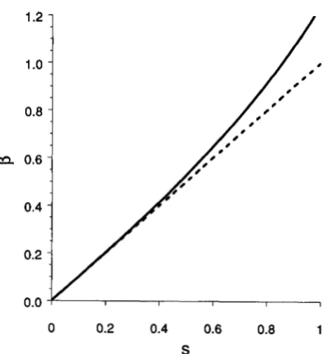
FIGURE 1.-The dependence of fi on s: the dotted line fi = s is compared with the numerical solution of the equation obtained from (20) and (22).

T h e derivative of this relative fitness curve at y = -1 is

which we can equate to s, according to

(20),

to determine @ in terms of s = U / r . T h e resulting equation can be solved numerically; but it is clear from Figure

1 that for any biologically reasonable s, e.g., s d 0 . 5 ,

which generalizes BARTON’S (1990) result ( l b ) for

k>>

1 to our more general selection model. In general, w ( y ) is not Gaussian; nevertheless, our Gaussian ap- proximation provides accurate predictions of apparent selection intensity, as shown by the numerical results below.

Environmental variance: T o simplify our presen-

tation, we have ignored environmental contributions to the quantitative trait. However, under the standard simplifying assumption that all genotypes experience identically distributed environmental perturbations with mean 0 and variance V E , our results need only a slight reinterpretation. The “phenotypic variance,” a

(7)

Bad Genes Meet Polygenes 609

on breeding values for 2 rather than phenotypes. Assuming that phenotypic selection has variance w2,

ie., W ( P ) = exp[-P2/(2w2)], V, = w2

+

VE (LANDE

1975). Our parameter /3 = d / V ,

=

V,/V, remains a sensible measure of apparent stabilizing selection. It

can be easily related to heritability and the intensity of stabilizing selection on phenotypes (see KEICHTLEY and HILL 1990) and to the index V,/VE discussed by

TURELLI ( 1 984).

NUMERICAL RESULTS

Our approximations are based on the assumption that the equilibrium distribution of the number of deleterious mutations per genome,

&k),

is approximately Gaussian after reproduction. We have found that under truncation selection with different U and truncation points, the deviation of g ( k ) from Gaussian depends mainly on

k.

With kabout 20, skewness and kurtosis of

&k),

measured by y 3 ( K ) = E [ ( K

-

k)’]/ui and y4(K) = E [ ( K

-

k)4]/ui

-

3, are about -0.01 and

0.30; and they tend to 0 as

k

increases (data not

presented). Genetically this means that reproduction with free recombination effectively destroys most of the higher-order disequilibria created by epistatic selection (TURELLI and BARTON 1990). Pairwise disequilibria, however, persist; because with synergistic epistasis u i

<

k

(KONDRASHOV 1984).

We are mainly interested in the distribution of 2 and the apparent fitness function. To determine the accuracy of our analytical approximations, we iterated numerically the equations described in KONDRASHOV

(1982) to obtain

&k).

We used a simplified model of

pleiotropy in which deleterious alleles have no effect on 2 with probability 1

-

Q, contribute + 1 with probability Q/2, or - 1 with probability Q/2. In the notation of the previous section, this corresponds to

a = 1 . For simplicity, we also assumed VE = 0. Figure

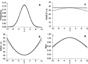
2 presents results for a population with U = 4 under truncation selection with T = 50. In this case,

k

=

and mutation load L = 0.431. Data for the trait are calculated with Q = 0.2.

Like

&k),

the distribution of phenotypes, p ( z ) , is very close to Gaussian with mean 0 and variance

kQ.

(Note that even if K has a Gaussian distribution and each (2

I

K = K ) is Gaussian, the population is composed of a mixture of Gaussians with different variances and

so will not be Gaussian.) Figure 2a presents the phenotypic distribution (uZ = 3.147, y3(Z) = 0, and y4(Z)

= 0.081) and a Gaussian distribution with the same

mean and variance. Our analytical prediction of W(z) is based on approximation (14) for E ( K

I

2 = z ) and the assumption that Var(K

I

2 = z) u i for all common phenotypes. Figure 2b compares predicted and observed values of E ( K 12 = z), and Figure 2c presents computed genotypic variances for different pheno-

49.508, UK = 5.777, y3(K) = 0.015, 74(K) = -0.020,

types. We can see that the analytical approximation for E ( K

I

2 = z) is quite good; and for most phenotypes, the conditional variance differs from &by only +5%.

We next consider apparent stabilizing selection. With truncation and similar selection regimes, the apparent stabilizing selection function is platykurtic

(if?., y4

<

0; under our assumptions, it is always

symmetrical, so that 7 3 = 0). Figure 2d presents the numerically determined apparent fitness function and the approximating Gaussian predicted from Equations

21 and 23. It is convenient to normalize the selection function, so that it can be treated as a probability density and characterized by its moments. T h e computed selection function has u = 9.564 and y4 =

-0.333, while the Gaussian approximation has u =

11.062. Despite this discrepancy, Figure 2d shows that

in the range where the phenotypic distribution is concentrated, the agreement between predicted and observed apparent fitnesses is nearly perfect. This suggests that the “variance” of the apparent fitness function is not a very useful measure. Although it works well when all of the functions are precisely Gaussian, it seems too sensitive to what happens outside the range +3uz.

T o illustrate this point, consider Figure 3, which presents data on calculated and estimated selection over a wide range of phenotypes, together with the phenotypic distribution. This figure assumes U = 2

and exponential-quadratic selection against mutations with (Y = 0.0 and /3 = 0.0012 [ie., s(k) = exp(-0.0006k2)]. At equilibrium,

k

= 42.945, UK =

6.427, ys(K) = 0.144, y4(K) = 0.019, and L = 0.660.

As before, we considered Q = 0.2. T h e small deviation of

i(K)

from Gaussian is caused largely by the discrete- ness of K ; note that the skewness and kurtosis are near what we expect from a Poisson with the same mean, i e . , y3 = 0.153 and y4 = 0.023. T h e phenotypic distribution has uz = 2.931 and y4(2) = 0.1 14. The predicted “standard deviation” of Gaussian selection,

u = 13.577, is smaller that the numerically computed

value u = 19.156 with y4 = -0.004. However, for phenotypes actually present in the population, the fitness curve is very close to the Gaussian with the analytically predicted u. Figures 2 and 3 show that the departure from the Gaussian fitness curve is mostly outside the range of common phenotypes, ie., beyond

+3uz. Our analytical approximation for

/3

predicts the

other indices of selection intensity much better than the value obtained from the numerically computed variance of the fitness curve (see Figure 5 below). Curiously, the main cause of the deviation of the apparent fitness curve from Gaussian seems to be the sixth moment. Letting y 6 ( x ) = E [ ( X

-

E ( x ) ) ~ ] / u $

-

15, y 6 ( x ) = 0 for a Gaussian, while our empirical distribution of apparent fitnesses gives 7 6 = -1.76,

(8)

610 A. S. Kondrashov and M . Turelli

0.14 7

-12 -8 -4 0 4 8 12

z

40

35

Y

30

g

20

25

Y

15

10 1 I I I

-12 -8 -4 0 4 8 12

z

48

1

0.00

7,

-12 -8 -4 0 4 8 12 -12 -8 -4 0 4 8 12

Z z

FIGURE 2.-Phenotypic distribution (a), p ( z ) ; the conditional mean number of mutations for different phenotypes (b), E ( K I Z = z); the conditional variances (c), Var(K I Z = z); and apparent stabilizing selection function (d), W ( z ) , calculated numerically for truncation selection with Ii = 4, T = 5 0 , V , = 0, Q = 0.2 and a‘ = 1. Numerical results are dots, and analytical approximations are presented as lines (see text for ;tdditional details).

1.20

1

.oo

0.80

0.60

N

0.40

0.20

0.00

0.2

0.1 6

0.12

z

-*

a

c

(D

3

0.08

yo

0.04

0

-50 -30 -10 10 30 50

Z

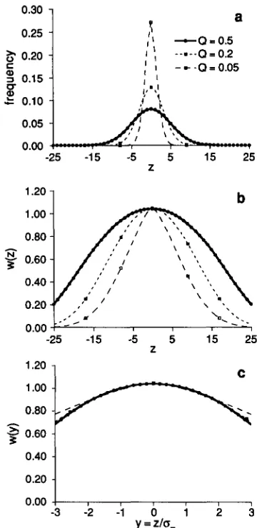
FIGURE 3.-Phenotypic distribution (open circles) and the analytically predicted (line) and numerically computed (dots) apparent fitness curves under exponential-quadratic selection (see text for details).

Our analytical approximations predict that the intensity of apparent stabilizing selection, as measured by

P,

does not depend on Q. Figure 4 presents phenotypic distributions and apparent fitness functions using the same model as in Figure 2 for various Q. Although the variance of the phenotypic distribution (Figure 4a) and the variance of the fitness function (Figure 4b) are proportional to Q, the fitness functions are practically identical when measured in units of

phenotypic standard deviations (Figure 4c). With Q =

1 and strict truncation, the fitness curve is jagged (data not presented). When Tis even, even phenotypes have enhanced fitness, with odd T , odd phenotypes have enhanced fitness. This artificial effect rapidly disappears with deviation from strict truncation, V E

>

0, and/or Q

<

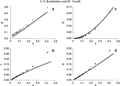
1.

Let us now consider the intensity of apparent selection. Figure 5 shows the dependence of

8,

the apparent genetic load ( L ) , the fitness variance (D), and the difference between the relative fitness of the “optimal” phenotype versus those one standard deviation away

( S ) on s = U/K. Two series of mutation-selection equilibria are considered: U =

2

and U = 6. For each, we

assumed truncation selection with T = 10, 20,

.

. .

,

100. Analytical predictions for /3 were obtained from the numerically determined s = U / k using (20) and

(9)

Bad Genes Meet Polygenes 61 1

0.30 -

0.25 -

-25 -15 -5 5 15 25

Z

1.20 1 _b

0.40

y

,;‘. , ,

‘.

‘’I I

0.20

I

0.00

-.

b.

I..

-25 -15 -5 5 15 25

Z

l . * O

1

C

::q

, , , , ,

,

0.00

-3 -2 -1 0 1 2 3

y = Z l b

Z

FIGURE 4.-Phenotypic distributions (a) and apparent selection curves, (b) before normalizing to the phenotypic standard deviations ;und (c) after normalizing, using the same selection model as in Figure 2 but with Q = 0 . 0 5 , 0 . 2 , and 0.5.

DISCUSSION

Our analysis suggests that pleiotropic effects of unconditionally deleterious mutations may account for substantial quantitative genetic variation and produce significant apparent stabilizing selection. T h e genetic variance maintained for a trait is kQa2, where k is the average number of deleterious mutations per genome and Qa2 is the variance of pleiotropic effects on the trait averaged over all deleterious mutations. T h e intensity of apparent selection, measured as

p,

the ratio of the genetic variance to the variance of the apparent fitness function, is close to s, the selection coefficient against individual deleterious alleles. Al- though we assumed that all deleterious mutations are equivalent, in the sense that fitness depends only on the total number of deleterious alleles carried, we allowed arbitrary directional selection against them. We have emphasized synergistic epistasis, which produces repulsion disequilibria among the deleterious alleles (i.e., a more even distribution of deleterious alleles across genomes than expected under independ-

ence). BARTON’S (1 990) results, obtained assuming multiplicative selection and complete linkage equilibrium, are identical if the number of deleterious alleles affecting the trait is large, i e . , =

Qk

>>

1. Our analysis implicitly assumes k T

>>

1 in approximation

(1 4) and by assuming that the sum (2) is approximately Gaussian. We will compare the HK model’s predictions with various data and discuss how our generali- zation of BARTON’S results might modify their inter- pretation.

Variance in quantitative traits: T h e result VC E

a; = &a2 = kTa2 requires only the conditional inde-

pendente

of allelic effects on the trait within individuals carrying a fixed number of deleterious alleles. This follows from our assumption that these allelic effects do not influence fitness. This would be violated if an allele’s effects on fitness and the trait were correlated, as assumed by KEIGHTLEY and HILL (1 990), or if selection acts directly on the trait.

It is unclear how much variation Vc = KQa predicts, since

k,

Qand a 2 are difficult to estimate. In particular, we do not know Qa2, the variance of phenotypic effects averaged over all deleterious mutations. This quantity translates the mean number of deleterious mutations into “phenotypic units.” T o our knowledge, the only relevant data appear in MACKAY, LYMAN and

JACKSON (1992), who examined the effects of P ele-

ment inserts on viability and abdominal and sterno- pleural bristle number in Drosophila melanogaster.

They estimated heterozygous effects of Qa2 = 0.003V~

per insert, which could account for significant variation if

k

is on the order of 100. However, we do not know if P element insertions are “typical” deleterious mutations.

Although our analysis assumes that the number of genes affecting a particular trait, i.e., =

KT,

is much larger than one, it is not clear what k T is consistent

with experimental data. Although very small values,

e.g., much less than one, would be inconsistent with high levels of additive variance, values of

KT

near 1 would be difficult to reject. Even though each individual might carry only one allele affecting the trait, this allele would occur at different loci in different individuals. Thus, selection could produce long-term changes in the mean phenotype and environmental variance could produce a continuous phenotypic distribution. With, say,

k =

100 (as suggested by CROW

1979) and Q = 0.1, each genome carries on average

10 mutations affecting the trait. With a 2 / V E s 0.1, which may be reasonable (e.g., FALCONER 1989, Table

12.2), this model could account for heritabilities near 0.5.

Obviously, pleiotropy can produce variance for many traits simultaneously. For fixed

k

and Q, one can imagine 100 traits with heritability 0.5 and only

-

(10)

612 A. S. Kondrashov and M. Turelli

0.5 -

0.4 -

0.3 -

0.2 -

0.1 -

a

‘

a

0.0 I I I I 1

0 0.1 0.2 0.3 0.4 0.5 S

0.30

0.20

b

1

0 0.1 0.2 0.3 0.4 0.5

S

0.1 0 -

0.08 -

0.04-

/

0.06 -

0.02

0.00 I I I I

0 0.1 0.2 0.3 0.4 0.5

S

0 0.1 0.2 0.3 0.4

9

1

0.5

FIGURE 5.-Different characterizations of apparent selection intensity plotted against s = U/R : fl (a); L , apparent load (b); D , variance in relative fitness (c); and S, the difference between the apparent fitness of the optimal phenotype and phenotypes one standard deviation away (d). Analytical predictions are solid lines, numerical values are open circles for U = 2 and dots for U = 6 (see text for additional details).

-

small pairwise genetic correlations. In this model, correlations arise from overlap in the deleterious mutations that affect two traits and correlations in their bivariate pleiotropic effects. Although shared devel- opmental pathways will ensure correlations between some traits (WAGNER 1989), selection against deleterious mutations might account for selection on a large number of essentially independent traits affected by different sets of loci.

Apparent stabilizing selection and actual genetic load: Our model implies that at mutation-selection equilibrium, the intensity of apparent stabilizing selection, as measured by

p,

is approximately s, the selection coefficient against individual deleterious alleles. Consequently, apparent stabilizing selection can be reasonably intense (e.g., /3

>

0.03) if s = 0.03

-

0.1 for deleterious mutations. Under our assumptions, s

can be represented as both U / r and UT/&. Other characterizations of selection intensity depend only on

,6 if the fitness curve and phenotype distributions are Gaussian (see Equations

7

and 8). Although our model does not produce precisely Gaussian fitnesses or phenotypes in general, our Gaussian-derived approximations for apparent load, variance in relative fitness, and differences between the apparent fitness of the mean phenotype versus phenotypes one standard deviation away are quite accurate (Figure 5 ) . Because even individuals with the “optimal” phenotype usually carry deleterious alleles, the apparent load computed from (6a) is always smaller than the actual one.

An alternative representation of

p

is instructive. Note that

where v = u/uK is the “genome degradation rate”

(KONDRASHOV 1984), and c = u i / r , which is between

0.5 and 1, quantifies the linkage disequilibrium produced by selection. At equilibrium, v = - & / U K ($

Equation 17), which equals the “intensity of selection” under truncation selection and determines the fraction of the population that survives (FALCONER 1989, Ch. 11). For fixed v , the intensity of apparent stabilizing selection decreases as u K / k , which is proportional to 1/&. This is because the apparent selection results from phenotypic variance increasing with K . As

u K / r + 0 when

k+

03, this effect disappears. On the

other hand, for fixed

r,

the strength of apparent selection increases approximately linearly with v . T h e increase is actually slightly slower than linear, because c, which depends mainly on v (KONDRASHOV 1984), decreases as v increases. However, this departure from linearity is small, because c is between 0.5 (v + m) and

1 (v + 0) under synergistic epistasis.

It is noteworthy that in this idealized model, the strength of apparent stabilizing selection does not depend on either Q or a’, because the parameter combination Qa‘ simply determines the scale of meas- urement for the trait ($ Equations 12 and 13). There- fore, we have only two parameters, r a n d either U or

(11)

Bad Genes Meet Polygenes 613

v , and the theory produces clear predictions concern-

ing the effects of each.

There is a negative trade-off between VC and

P

in this model, because VcP r (cQa2)(U/k) = UQa2 = U T a 2 . Under multiplicative selection, the mutation load is 1

-

exp(-U), which constrains U to be smaller than 1 or 2 (CROW 1970). This fact, among others, led BARTON (1 990) to conclude that “mutation-selection balance is an unlikely cause of quantitative variation” (p. 779). However, this constraint is essentially eliminated by synergistic epistasis. Under truncation o r similar selection regimes (CROW and KIMURA

1979)) mutation load depends not on U but on the genome degradation rate v = U/uK. By calculating the fraction of the population that must be “culled” to produce selection intensity v , one sees that the mutation load becomes intolerable only for v

>

2 (corresponding to less than

5%

survival under truncation selection, ignoring nongenetic sources of mortality).

For v d 2, the load remains reasonable even for arbitrarily large U (KONDRASHOV 1984, 1988). Be- cause IJK 3

*

even under strong synergistic epistasis (Equation I), v = u / U K

c

2 whenever

u2/2.

Consequently, for fixed U , load constraints imply only that Vc 3 QU2a2/2 and s d 2/U. These are not significant restrictions when U

<

20-30. For instance, with

U = 5 ,

r=

100, and Q = 0.1, our model implies Vc =

loa2 and

P

s 0.05, so that both quantitative variance and apparent stabilizing selection can be substantial. T h e question is, however, whether the data on deleterious mutations and quantitative variance are com- patible with this model.

Data on mutation-selection equilibrium for dele-

terious alleles: Despite its enormous theoretical sig-

nificance, data relevant to mutation-selection balance for deleterious alleles are scarce. MUKAI et al. (1972) suggest U 1 .O; but this is probably an underestimate, particularly because: a) some slightly deleterious mutations may have been neglected, b) these data concern only one component of fitness, viability, and c) larval viability was measured under simple laboratory conditions, which may mask many mutations affecting viability in nature (see SIMMONS and CROW 1977;

CROW 1979; CROW and SIMMONS 1983). Recently, D.

HOULE, B. CHARLESWORTH and collaborators (per-

sonal communication) obtained higher estimates for

U by considering all fitness components. For mam- mals, data on mutation rates per nucleotide and molecular evolution imply about 100 new mutations per diploid genome per generation; but the deleterious rate U is an unknown fraction of this, equal to the fraction of genome constrained by selection (see KON-

DRASHOV 1988). For Drosophila, molecular evolution-

ary rates of about 10-8-10-7 per nucleotide per year have been reported (CACCONE, AMATO and POWELL 1988; ROWAN and HUNT 199 1). With diploid genome

size about 3 X lo8 bp and several generations per year, this suggests U = 0.1-2.0, if we assume arbitrar-

ily that about a third of all DNA can produce deleterious effects. However, data on rates of molecular evolution may significantly underestimate mutation rates because of purifying selection which apparently influences the majority of Drosophila scnDNA (CAC-

CONE, AMATO and POWELL 1988) and can operate outside transcribed regions (COHN and MOORE 1988; LI and SADLER 1991). CHARLESWORTH, CHARLES-

WORTH and MORGAN (1990) estimate U

=

1 from

inbreeding depression in highly selfed plants. Overall, the scanty data for multicellular eukaryotes are consistent with any value of U between 0.1 and 100.

T h e mean equilibrium number of slightly deleteri-

ous mutations per genome and the average selection coefficient against them are not known with any con- fidence for any species. T h e best estimates for Dro-

sophila are

k

2 50 and s s 0.02 (the estimate of s is the harmonic mean and the estimate of

k

assumes

U z 1; CROW 1979), but they both are likely to be underestimated. MACKAY, LYMAN and JACKSON (1 992) found deleterious heterozygous fitness effects of 0.055 per P element in a homozygous genetic background. As they noted, their inserts could produce significant apparent stabilizing selection.

Transposable elements may account for a substantial proportion of the deleterious mutations we discuss. They comprise about 10% of the

D.

melanogaster

genome, with on the order of 103-104 individual elements per genome (BINGHAM and ZACHAR 1989). They are apparently deleterious, and their copy number seems to be controlled by some form of mutation- selection balance (CHARLESWORTH and LANGLEY

1989). In

D.

melanogaster, the total genomic mutation rate caused by transposable elements may exceed 1 (W. R. ENGELS, personal communication), and many of these mutations are deleterious. Moreover, they contribute to observed quantitative variation

(MACKAY AND LANGLEY 1990).

Nevertheless, these transpositions probably make only a small contribution to apparent stabilizing selection. T h e genomic mutation rate caused by transpositions equals the per-element transposition rate times the copy number. Thus, according to (23), the intensity of apparent stabilizing selection they produce should equal the per-element transposition rate. For different transposable elements, the estimates of “nor- mal” transposition rate vary from about (CHAR-

LESWORTH and LANGLEY 1989) to about 0.03 per

element per generation (PRESTON and ENGELS 1984). However, the latter figure is for the unusually mobile

P elements; and current data suggest that the average for all elements is unlikely to exceed lo-’ (CHARLES-

(12)

MUKAI 1990). Thus they would produce only very weak apparent selection.

Data on quantitative traits: Although the scanty

data on deleterious mutations may be consistent with explaining quantitative variation and apparent stabilizing selection, much stronger constraints emerge from considering parameters associated with quantitative genetic variation. In our notation, V,, the amount of new genetic variance for trait 2 introduced per zygote by mutation each generation (CLAYTON and ROBERTSON 1955), is UQa (cf. Equation 9b). On the other hand, Vc = TQa’. Hence, our analysis, like BARTON’S (1 990), implies that

Le., the intensity of apparent selection is approximately equal to the ratio of the variance introduced

by mutation each generation to the equilibrium genetic variance. This ratio can be estimated either directly from experiments concerned with the buildup o r maintenance of variation, or indirectly from the rate of long-term selection response (HILL 1982;

MATHER 1983; LYNCH 1988). Some studies estimate

V,/V, rather than Vm/VG, but these should not differ from

p

under our model by more than a factor of 5 given that heritabilities for the traits examined are typically between 0.2 and 0.6.

Although data on V,,,/Vc are not abundant, the consensus estimate for

D.

melanogaster bristle numbers is about (LANDE 1975; HILL 1982; MATHER

1983; MACKAY et al. 1992), an order of magnitude too low to explain appreciable apparent stabilizing selection. Similar values were obtained for Daphnia (LYNCH 1985), although the loss of many lines might have led to underestimation. In some other cases, however, values of V m / V , as high as 0.01-0.05 have been reported (see LYNCH 1988; KEIGHTLEY and HILL

1992). Hybrid dysgenesis can produce much higher values (MACKAY, LYMAN and JACKSON 1992), but this situation is not typical.

Thus, the highest estimates of V,/Vc are consistent with fairly strong apparent stabilizing selection; but the lowest estimates, and in fact most estimates, (corresponding to

p

= 0.001 or even 0.0001) imply neg- ligible selection. This may well reflect a real difference between the factors causing quantitative variation vs. stabilizing selection in nature, but more data on different organisms and traits are necessary. In some cases, very strong stabilizing selection has been reported (see ENDLER 1986), corresponding to

p

= 0.1 o r more under our model. Although this is not pre- cluded by load considerations, it is difficult to reconcile with most estimates of V m / V c . If additional studies find small values of Vm/VG, the mechanism considered here must be abandoned as the explanation for signif-

icant stabilizing selection, unless our simplified analysis overlooks something that dramatically modifies (23) and (25)

(4.

BARTON 1990). It is possible, however, that Vm has been substantially underestimated if mutations are deleterious and selection is not completely excluded during their accumulation (MACKAY

et al. 1992).

Because @ does not depend on Q under our model, data on UT = UQ, the total mutation rate to alleles contributing variation to the trait considered, are relevant only to explaining VG. Estimates from Dro- sophila, maize and mice imply U T = 0.01-0.1 (see

TURELLI 1984, 1988). With U = 3, this means that Q = 0.03-0.003, so that Ka2/V, must exceed 100 to maintain substantial heritable variance. However, these parameters would produce an s too small to account for significant apparent stabilizing selection. Although U T may well have been underestimated if

mutations with small contributions were not counted, even estimates as low as 0.01 are difficult to reconcile with traditional estimates of per-locus mutation rates and numbers of loci underlying quantitative variation

(cf. LANDE 1988; TURELLI 1984, 1988).

Direct us. pleiotropic mutation-selection balance

models: Direct-selection models assume that the al-

leles producing trait variation experience selection only from stabilizing selection acting directly on the trait. T o compare them to our pleiotropy model, we will use the “rare alleles” (house of cards) approximation (TURELLI 1988)) where, as in our HK model, all alleles contributing significant variation are rare at each locus.

T h e main result from one-trait, direct-selection models is VG E ~ U T V , . Here V, is a parameter describing direct stabilizing selection, and the question ad- dressed is “How much variance can be maintained?” In contrast, with the HK model, both Vc and V,

depend on selection extrinsic to the trait, and a central question is “What is their ratio

p,

i.e., what is the intensity of apparent selection?” Under direct stabilizing selection, the intensity of stabilizing selection, in units of VG, is

p

= VG/V, = 2uT. In contrast, our HK model gives

p

= s = U T / & . Given that

TT

must exceed

1 in biologically reasonable situations, we can conclude that for fixed U T , direct selection models will generally entail more intense stabilizing selection ( i e . , larger

0)

than the apparent selection produced by our pleiotropic model. However, the variance prediction of the HK model seems far more robust. Pleiotropy tends to reduce equilibrium genetic variance under direct-selection models by an amount that is difficult to predict (TURELLI 1985; WAGNER 1989; SLATKIN and FRANK 1990), whereas it is an inherent feature of