Statistical Characterization VBR MPEG at the Slice Layer
Michael R. Izquierdo Douglas R. Reeves
[email protected] [email protected]
(919) 543-0104 (919) 515-2044
Department of Electrical and Computer Engineering North Carolina State University
Raleigh, North Carolina 27695 fax: (919) 543-6552
July 29, 1994
Abstract
We studied the ATM cell-generation statistics of three VBR encoded MPEG video sequences at the Slice layer. Each of the video sequences contained Intracoded (I), Predictive-coded (P) and Bidirectional-coded (B) frames and included special camera effects such as zooming, panning and sudden scene changes. Each sequence consists of 150 frames at a rate of 30 fps. Previous research characterized sequences which did not include B frames. This was due to its long encode time making it unattractive for real-time video applica-tions. We examined video sequences with B frames since they offer the highest amount of compression and increased bit-rate variation which can be exploited when multiplexing multiple video streams. Also, it is likely that applications where video is stored for retrieval will contain B frames. The motivation behind studying the cell generation process at the Slice layer is that the slice size makes it well suited for transport packet payloads. It would be feasible to have ATM Convergence Sublayer (CS) payloads consisting of slices where destination nodes can detect slice errors and provide corrective action or attempt error concealment. Also, characterization at the Slice layer captures the spatial behavior of each frame.
1.0 Introduction
The Asynchronous Transfer Mode (ATM) Network has gained much attention as an effec-tive means to transfer voice, video and data information over computer networks. The use of a fixed size, fifty-three byte cells to transfer data makes ATM well suited to support iso-chronous type services like voice and video 1]. The small cell size makes it possible to interleave cells from other sources over a common communications link, thereby provid-ing low end-to-end latency. The transport of video data over ATM networks has been a fertile area of study. Specifically, much work has been done in the area of the transport of compressed video over ATM, addressing such issues like bandwidth allocation, model-ling, multiplexing, encoding methods (CBR vs. VBR), QoS1, etc. We attempt to address some of these issues in this paper by investigating the transport of MPEG-1 VBR encoded video over ATM.
We define a method of transporting video using ATM AAL-5 where Convergence Sub-layer (CS) packets are built from MPEG-1 Slices. In this paper, we use an MPEG-1 Video Packet Elementary Stream (VPES) which does not contain audio. In order to understand the impact this data stream will have on the ATM network, we statistically characterized three MPEG-1 encoded video sequences at the Slice Layer. The majority of work has dealt mainly with characterizing video at the Frame Layer which is a natural encoding bound-ary. However, we believe that error recovery and possibly forward error correction (FEC) are best done at the Slice Layer rather than the Frame Layer.We chose the Slice Layer because it is the lowest independent data unit in MPEG and does not require any data from any other Slice within a Frame for decoding. This makes it possible to provide error-detec-tion, correction or concealment on a portion of a Frame rather than the whole Frame. We use a model of a video server, shown in Figure 1, which sends ATM AAL-5 type CS packets over an ATM network to a video client. The video server parses the video stream in accordance to the MPEG-1 syntax and builds AAL-5 CS packets from MPEG Slices. Non-Slice data, such as Sequence Layer headers, are placed in its own CS packet. AAL-5 packets are segmented into 53 byte cells with each cell consisting of 48 bytes of video data payload. Cells are transported over the ATM network to a video client which reassembles the CS packet and checks for any errors. The error recovery mechanism would be con-tained in the video client. One possible example of an error recovery mechanism would be a Reed-Solomon FEC scheme where a CS packet could be corrected when a cell was either dropped or corrupted by the network. We focus our attention on the video server cell
stream output into the ATM network. We assumed zero delay between the generation of CS packets, since the assumption was that video data was immediately accessible from a local file system located on storage media.
.
We studied three video sequences, obtained from the Stanford University FTP1 archive, called Bike, Flowg and Tennis. We used the software decoder from the University of Cali-fornia at Berkeley called mpeg_play to view the video sequences and study their content. Each video sequence was VBR encoded with a quantization scale (q) triplet of (4,4,8). This means that q was set to 4 for I and P anchor frames and 8 for B reference frames. The video sequences were considered to be high quality encoded. All sequences contained 150 frames and had an Interframe-to-Intraframe ratio (M) equal to 2. We developed a program, written in C, which parses an MPEG-1 stream and extracts Slice and Frame data. The pro-gram also extracts and decodes all Sequence, Frame and Slice header information. Matlab 4.0 was then used to analyze the Cells/Slice data.
We calculate metrics such as the mean picture density and compression ratio to gain an understanding of the effectiveness of MPEG-1 encoding on different scene content and how they relate to the statistics. This was possible because each sequence was encoded using the same quantization values. We calculate statistics such as peak-to-mean ratio (PMR), coefficient-of-variation (CV) and autocorrelation in order to understand the
MPEG Parser
ATM Segmenter Slices
ATM Cells
Queue
MPEG ATM
Network
Traffic Rate Enforcement Cells
Slice Number Cell Generation Statistic
Output Rate, R
FIGURE 1. VBR video server model to analyze cell generation statistic
amount and behavior of the variability in the data.We compare the probability mass func-tion (pmf) of each of the video sequences to the Gamma distribufunc-tion by using the QQ plot. Recent papers have shown that MPEG sequences with only I/P frames fit the Gamma dis-tribution well. We try to determine if this is also true for video sequences with I/B/P frames.
We introduce a multiplexing scheme, for VBR video with I/B/P frames, which we call
Time-Shifted Multiplexing (TSM) which attempts to take advantage of the periodicity we
found in I/B/P video sequences. We show a model of each of the sequences based on an 8-state discrete-time, discrete-8-state Markov Chain where each 8-state represents a range of Cells/Slice values. The number of states was chosen to be approximately equal to the number of standard deviations between the peak and the minimum number of Cells/Slice. Finally, we discuss the impact of I/B/P sequences on dynamic bandwidth allocation schemes
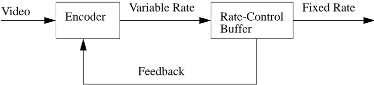
1.1 VBR vs. CBR
There are two basic methods to encode video: variable rate (VBR) and constant bit-rate (CBR). VBR encoders attempt to keep the video quality constant by not changing the quantization scale in order to maintain constant bit rate output. VBR encoded video trade-off constant bit-rate output for constant video quality. This variation in output bit-rate pre-sents more of a challenge for computer networks in terms of bandwidth allocation and guarantees for QoS such as cell loss. The CBR encoding technique attempts to remove the variability of the video stream by varying the picture quality. This scheme requires a rate-control buffer at the output of the encoder, shown in Figure 2, where the quantization level is changed when the rate control buffer approaches an underflow or overflow condition. As the buffer approaches an overflow condition, the bit-rate is reduced by increasing the quantization level. When an underflow condition is detected, the bit-rate is increased by decreasing the quantization level. This variation in video quality is an undesirable effect of encoding video using the CBR method. However, transmitting video using CBR makes it easier to request bandwidth when establishing an ATM connection.
achieved by statistically multiplexing multiple VBR sources. Verbiest, et al. [3] has shown that the statistical multiplexing of multiple VBR sources provides a gain of a factor of two over multiple CBR sources.
1.2 VBR Video Transport
One of the main drawbacks of transmitting compressed video using VBR is that the prob-ability of cell-loss can increase when transporting cells over ATM networks. This is caused by the variability in the cell stream where the source exceeds the allocated band-width. The user must specify its bandwidth requirements when establishing a connection in order for the network to determine if enough resources exist. This method is a preventa-tive congestion control technique in that flow control is done at the source prior to conges-tion [4]. The user can specify a bandwidth allocaconges-tion at the peak rate; however, this would not be an efficient utilization of bandwidth.
Dropping cells from the video stream without regard to content can cause serious degrada-tions in picture quality. MPEG-1 was developed to operate over lossless connecdegrada-tions and does not define a transport protocol1 to deliver compressed video data over networks. As a result, several techniques have been developed to either reduce the effects of cell-loss with VBR video sources or minimize the amount cell-loss.
1.2.1 Two Layer Codecs
A two-layer codec is used to reduce the effects of cell-loss by dividing the encoder output into two streams [5], [6]. The first stream is produced by the Base Layer and is a CBR
1. SNR is used as a measure of video quality and is computed as the mean square error between the input pixels to the encoder and the decoded output.
1. This has recently changed with the announcement of the MPEG-2 draft standard which defines Transport
Encoder Variable Rate Rate-Control Buffer
Fixed Rate
Feedback Video
stream consisting of high priority cells transported over a lossless, or high quality, connec-tion. The second stream is produced by the Enhancement Layer and is a VBR stream con-sisting of low priority cells transported over a lossy connection. The Base Layer contains the basic structural information of the picture while the Enhancement Layer contains the difference between the input stream and the decoded output of the Base Layer. When traf-fic exceeds the allocated bandwidth, the network will drop low priority cells from the Enhancement Layer in order to prevent network congestion. Both streams are combined at the decoder in order to reproduce the video stream.
The two-layer codec makes the video stream more resilient to cell-loss. Morrison [2] indi-cated that a one-layer codec must operate with cell losses not greater than 10-5before a degradation of quality is visible. However, for two-layer codecs it is possible to operate with cell loss rates at 10-3. Kishino, et. al. [7] compared one-layer encoded pictures, where cells were dropped at random, to pictures which were two-layer encoded and low priority cells were dropped. The results showed that the quality of the one-layer encoded picture with random cell-loss at a rate of 5% was significantly worse than a two-layer encoded picture with 50% loss of low priority cells.
1.3 Dynamic Bandwidth Allocation
Another technique, called Dynamic Bandwidth allocation, tries to prevent cell-loss by changing the allocated bandwidth during a connection by predicting that additional band-width will be required in the near future based on the recent behavior of the traffic stream. This scheme requires a fast-reservation protocol (FRP) [8] to reserve extra bandwidth upon request. The unit which monitors the traffic and requests additional bandwidth is referred to as the Traffic Predictor. One example of this technique was proposed by Pan-cha, et. al. [9] which allocates bandwidth at the mean rate when a connection is established and increases or decreases bandwidth by one standard deviation based upon the bit-rate behavior of the source. This requires full statistical characterization of the video stream in order to calculate the mean and standard deviation. A Markov-chain was used to show that the probability of the bandwidth changing by more than one standard deviation was ineli-gible. We will show that while this is true for sequences containing I/P frames is not the case with sequences containing I/B/P frames.
where each state represents a rate class. Traffic is monitored by a video control unit which uses a unique policing algorithm to ensure the traffic does not exceed the bit-rate of the rate class. If this occurs, the video control unit can temporarily switch the video traffic to a higher rate class. One can see a similarity between this technique and that proposed by Pancha, et al. in that if the rate classes where separated by one standard deviation then the bit-rate jumps would be equivalent.
2.0 MPEG-1 Overview
The MPEG -1standard was submitted for approval to the ISO-IEC/JTC1 SC29 standards body in November of 1991. The standard was prepared by the SC29/WG11 committee also know as the Motion Picture Experts Group (MPEG). The standard is divided into four parts titled: (1) ISO/IEC 11172-1 Systems, (2) ISO/IEC 11172-2 Video, (3) ISO/IEC 11172-3 Audio and (4) ISO/IEC 11172-4 Conformance Testing. This paper specifically deals with 11172-2 Video [11] part of the standard.
The MPEG compression algorithm is asymmetric in that it takes much more time and compute power to encode video than to decode it. Asymmetric techniques are well suited for situations where video data is compressed off-line and stored for future play-back. The objective is to make the decoders simple and inexpensive. A good overview of MPEG is found in DeGall [12]. In symmetric video compression algorithms, the encode/decode computational burden is balanced which shifts some of the encoder complexity to the decoder. This makes the encoder less expensive and the decoder more expensive. The time it takes to encode video decreases as well.
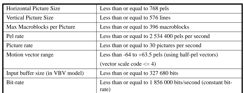
The standard defines constraints, shown in Table 1, on the format, encoding and decoding parameters of the video stream. A video bit stream which adheres to the constrained parameters is referred to as a Constrained Bit Stream (CPB). The actual syntax of the MPEG bit-stream allows for values greater than the constrained parameters; however, adhering to CPB sets limits on the bandwidth, buffer sizes and memory bandwidth. MPEG videos typically come in two Standard Interface Formats (SIF) dimensions: 352x240 pix-els @ 30 fps (330 macroblocks/picture1 maximum) and 352x288 pixels @ 25fps (396 macroblocks/picture maximum).
.
2.1 MPEG Compression Technique
MPEG essentially relies on two techniques for compression: block-based motion compen-sation which takes advantage of temporal redundancy and discrete cosine transform (DCT) which takes advantage of spatial redundancy. There are two types of motion com-pensation used in MPEG: prediction and interpolation. Prediction assumes that the current picture block can be created from a past or future frame’s picture block. Interpolation ref-erences picture blocks from both a past and future frame and uses a mathematical combi-nation of the two (usually the average) to create the current picture block. This method is usually computational intensive, but provides the most compression.
2.1.1 Spatial Compression
In MPEG, spatial compression is accomplished by using the two-dimensional Discrete Cosine Transform (DCT), quantization and run length coding. Frames which use spatial compression solely are referred to as Intracoded frames or I frames. The DCT operates on an 8x8 matrix of pel values called a Block. The DCT translates the time domain represen-tation of the Block into the frequency domain and outputs a DC coefficient and a number of AC coefficients. The Inverse Discrete Cosine Transforms (IDCT) converts the block from the frequency domain back to the time domain. The two-dimensional DCT, and the IDCT, are shown below.
Horizontal Picture Size Less than or equal to 768 pels
Vertical Picture Size Less than or equal to 576 lines
Max Macroblocks per Picture Less than or equal to 396 macroblocks
Pel rate Less than or equal to 2 534 400 pels per second
Picture rate Less than or equal to 30 pictures per second
Motion vector range Less than -64 to +63.5 pels (using half-pel vectors)
(vector scale code <= 4)
Input buffer size (in VBV model) Less than or equal to 327 680 bits
Bit-rate Less than or equal to 1 856 000 bits/second (constant bit-rate)
TABLE 1. Summary of Constrained Parameters
F u v( , )
The value of the coefficient is divided by the quantizer step and rounded to the nearest whole number.
The DC coefficients of the luminance and chrominance blocks are coded using a Differ-ential Pulse Code Modulation technique (DPCM) in which the DC coefficients of the cur-rent block are subtracted from the preceding block with the result used. A Variable Length Code1 (VLC) is then used to represent the absolute value of the result which differ for luminance and chrominance. The DC coefficient of the first macroblock within a Slice is an absolute value which makes Slices independent from each other. One can see that if the first macroblock within a Slice is corrupted, the whole Slice could decode erroneous DC coefficient values. If a macroblock towards the end of a Slice were corrupted only those macroblocks which follow will have their DC coefficients corrupted.
AC coefficients are Run Length Coded (RLC) using a combination of the Run-Length and Level code. The Run-Length value is the number of zero AC coefficients skipped between non-zero coefficients. The non-zero AC coefficients are specified using the Level code. This technique takes advantage of the fact that most of the AC coefficients are zero.
2.1.2 Temporal Compression
Temporal compression is accomplished by using a motion compensation technique. Frames which employ motion compensation are referred to as Intercoded frames. Motion
1. Variable Length Codes use fewer bits to represent data which occurs with high frequency and more bits to represent data which occur with low frequency. Since the luminance does not differ greatly between adjacent
f x y( , ) 1
4 C u( )C v( )F u v( , )
2x+1
( )uπ
16
2y+1
( )vπ
16 cos cos
v=0 7
∑
u=0 7
∑
=
F u v( , ) 1
4C u( )C v( ) f x y( , )
2x+1
( )uπ
16
2y+1
( )vπ
16 cos cos
y=0 7
∑
x=0 7
∑
=
C u( ),C v( ) 1
2
= for u v( , ) = 0
compensation achieves video compression by sending a reference pointer or motion vec-tor to a past or future picture block instead of sending the DCT coefficients. In almost all cases, sending a pointer to a past or future picture block requires less bits than sending the actual coefficients. Motion compensation is block based in that a 16x16 pel area of the current picture is used to match against a past or future block. If an exact match is found, only the pointer is sent. If a close match is found then the difference between the two blocks is sent along with the pointer. If an exact match is found with a block in the same position, no pointer is sent and the block is skipped by specifying a skip-indicator. The skip-indicator tells the decoder to use the values of the block contained in the past picture in the current position.
There are basically three types of motion compensation used in MPEG: forward-predic-tive, backward-predictive and bidirectional-predictive. Forward-Predictive motion com-pensation tries to match blocks from a past frame, whereas Backward-Predictive tries to match blocks from a future frame. Bidirectional-Predictive motion compensation tries to match blocks from both a past and future picture and then uses an mathematical method (typically the average) in order to synthesize the current block. This technique is referred to as interpolation. Block matching can be exhaustive in that all blocks within a frame are searched; however, typically a specific search area is specified for encoding (e.g. +/- 16 pels or +/- 7 pels).
2.2 MPEG Layered Structure
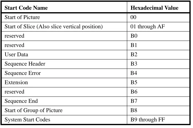
The standard specifies the syntax for compressed video streams and consists of six layers which are listed in Table 2. Each layer is identified within the video stream by a Start Code Prefix followed by a unique Start Code listed in Table 3. All layers, except for the Block1 Layer, contain header information. The layering approach allows for the efficient parsing of the compressed video bit stream which is required to support random access, forward and reverse picture scanning, picture editing and error recovery.
2.2.1 Sequence Layer
2.2.2 The Sequence Layer begins with a header followed by one or more Group-of-Pictures (GOP) and ending with an End-of-Sequence code. Each GOP may be preceded by a sequence header. The sequence header contains video information such as the horizontal and vertical picture sizes, pel aspect ratio, picture rate, bit rate, and virtual buffer verifier (VBV) size.
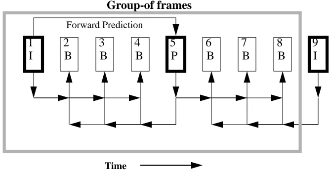
2.2.3 Group-of Pictures Layer
A GOP consists of a collection of pictures. A typical format for a GOP is shown in Figure 3. Each GOP contains at least one I frame. B frames within one GOP can reference an I frame in another GOP. The ratio of Intercoded-to-Intracoded pictures (N) is equal to the number of B/P frames divided by the number of I frames.
Layers of Syntax Function
Sequence Layer Random access: context
Group of Pictures Random access unit: video
Picture Layer Primary coding unit
Slice Layer Resynchronization unit
Macroblock Layer Motion Compensation unit
Block Layer DCT unit
TABLE 2. Structure of MPEG bit stream
2 B
3 B
4 B
5 P
6 B
7 B
8 B
9 I 1
I
Forward Prediction
FIGURE 3. MPEG temporal picture structure N=7 Time
2.2.4 Picture Layer
There are four type of frames in MPEG: Intracoded (I), Predicted (P), Bidirectional-Pre-dicted (B) and DC frames. I frames are encoded using DCT and IDCT and do not use motion compensation and are referenced by P and B frames. P frames reference a previous I or P frame by using motion compensation. B frames are coded with reference to the pre-vious I or P frame, next I or P frame or both. B frames use motion compensated interpola-tion. DC frames are encoded using DCT and IDCT, but only use the DC coefficients. This provides a simple, but low quality fast-forward mode. None of the video sequences stud-ied in this paper contained DC pictures.
2.2.5 Slice Layer
Each picture is divided into Slices consisting of a Slice header and one or more macrob-locks. The Slice header contains the vertical position of the slice within a picture and the quantization scale (q) since Slices can have different quantization scales. Each Slice is encoded without dependence on any other Slice. As a consequence, a Slice is the lowest error-recoverable unit within MPEG. If an error occurs within a Slice, it is possible to recover from the error and not affect the total picture.
The number of Slices per frame is quite flexible and is determined during encode time. A frame can consist of Slices which start at the left side of the picture and end at the right hand side as shown in Figure 41. An alternate format would be to make the Slice start on one horizontal line of the picture and end on another. This is shown in Figure 5. It is possi-ble for a picture to contain only one Slice; however, if an error occurs then the whole pic-ture is affected. The benefit of reducing the number of Slices within the picpic-ture is in reducing the header overhead associated with each Slice.
Each Slice consists of a 40 bit header; consequently, the more Slices per picture, the more header bits within a picture. If the video sequence is transported over a very reliable net-work then this trade-off is acceptable. However, this is not acceptable for VBR video sequences on ATM networks where the likelihood of causing a Slice error due to cell-loss exists. Therefore, a format which divides the picture into multiple Slices is preferable for VBR transmission.
.
2.2.6 Macroblock Layer
The macroblock is the basic unit of coding for motion compensation. Macroblocks are encoded from the top left-most part of the picture to the lower right-most part scanning from left-to-right and top-to-bottom. Macroblocks consists of a header followed by six component blocks shown in Figure 6. The six component blocks are made from four lumi-nance blocks (Y) and two chromilumi-nance blocks Cr and Cb1.
FIGURE 4. Possible Slice arrangement for SIF 352x240 picture. 1 Begin 2 Begin 3 Begin 4 Begin 5 Begin 6 Begin 7 Begin 8 Begin 9 Begin 10 Begin 11 Begin 12 Begin 13 Begin 14 Begin 15 Begin 1 End 2 End 3 End 4 End 5 End 6 end 7 End 8 End 9 End 10 End 11 End 12 End 13 End 14 End 15 End
FIGURE 5. Alternate Slice arrangement for SIF 352x240 picture. 1 Begin 2 Begin
3 Begin 4 Begin
5 Begin
6 Begin 7 Begin 8 Begin 10 End 12 End 1 End 2 End 3 End 4 End 5 End 6 end 13 End 7 End
8 End 9 Begin 9 End 10 Begin
11 Begin
11 End 12 Begin 13 Begin
0 1
2 3 5 6
Y Cr Cb
The macroblock header contains the macroblock stuffing, address increment, macroblock type, and quantization scale (q) fields. Macroblock stuffing is used by the encoder to increase the bit-rate of the data stream in order to avoid a buffer underrun condition. These bits are discarded by the decoder. The macroblock address increment defines the relative position of the macroblock within the current Slice. Macroblocks which are intracoded always have an address increment of 1. Intercoded macroblocks can have an address increment greater than 1 and are called skipped macroblocks. The quantization scale is used to calculate the quantization step for the current macroblock. This is an adaptive quantization technique in that the quantization scale can be different for each macroblock. The quantization step limits the range of values of the DCT coefficients. For DC coeffi-cients it is fixed at 8, but for AC coefficoeffi-cients it is calculated using the following formula:
In this formula, i[u,v] is the quantized coefficient matrix, c[u,v] is the coefficient matrix, and m[u,v] is the quantization matrix. The quantization matrix could be a default matrix or downloaded in the sequence header. The output bit-rate of the encoder can be varied by changing the quantizer step. This is done by changing q in either the Slice or macroblock headers.
There are four basic types of macroblocks in MPEG: Intracoded, Forward-Predictive, Backward-Predictive and Bidirectional-Predictive. Intracoded macroblocks (I) use spatial encoding and do not reference any other frame. Forward-Predictive macroblocks (P) use motion compensation and contain a motion vector which points to a macroblock in the previous I or P frame. Backward-Predictive macroblocks (B) contain a motion vector which points to a macroblock in the next I or P frame. Bidirectional-Predictive macrob-locks use interpolation and contain two motion vectors which point to macrobmacrob-locks in the previous and next I or P frames.
The picture type determines the types of macroblocks contained within the frame. For example, I frames only contain I macroblocks while P frames contain both I and P mac-roblocks. The motion compensation unit must go through a decision process in order to determine which macroblock type to select. The decision as to which macroblock type to
1. This is referred to as the 4:2:0 format as opposed to the 4:2:2 format which uses two chrominance blocks or a 4:4:4 format which uses four chrominance blocks. MPEG-1 only uses the 4:2:0 format; whereas, MPEG-2 specifies the 4:2:2and the 4:4:4 format.
select is roughly based on which one will require the fewest bits to encode. If an appropri-ate motion vector is found then the macroblock is encoded as a P macroblock; otherwise, it is encoded as an I macroblock. B frames are the most complex and consist of all four macroblock types. They require the most computing power to encode, but offer the highest amount of compression.
2.2.7 Block Layer
The Block is the lowest layer in the MPEG architecture. It is the basic coding unit for the DCT/IDCT spatial compression algorithm. Each block consists of 64 pels arranged in an 8x8 structure.
2.3 Start Codes
The MPEG bit stream is delimited by the Start Code Prefix and Start Code shown in Figure 3. The Start Code Prefix is a 001 byte pattern which does not occur normally in the bit stream. Once the decoder detects a Start Code Prefix it then decodes the next byte which is the Start Code. Following each Start Code is header information pertaining to that particular layer.
Start Code Name Hexadecimal Value
Start of Picture 00
Start of Slice (Also slice vertical position) 01 through AF
reserved B0
reserved B1
User Data B2
Sequence Header B3
Sequence Error B4
Extension B5
reserved B6
Sequence End B7
Start of Group of Picture B8
System Start Codes B9 through FF
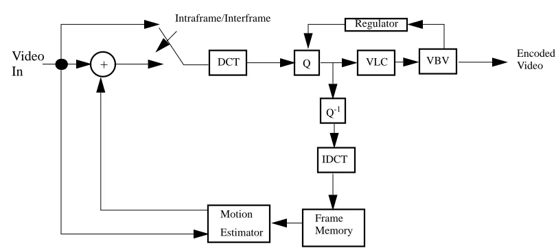
2.4 MPEG Encoder
A simplified diagram of the MPEG encoder is shown in Figure 7. During Intraframe cod-ing, the DCT, Quantizer (Q) and Variable Length Coding (VLC) is used to compress a macroblock. The Inverse Quantizer (Q-1) and the Inverse Discrete Cosine Transform (IDCT) are used to develop the frames for reference by motion compensation. The bit-rate is assumed to be constant and is specified in the sequence header.
The Virtual Buffer Verifier (VBV), shown at the output of the encoder, is a buffer moni-tored by the Regulator to insure that an overflow or underflow condition does not occurs. If the VBV is approaching an underflow condition, stuffing bits are added by specifying a macroblock stuffing code in the macroblock header. These stuffing bits are removed at the decoder. The stuffing bits effectively increase the bit-rate of the encoded output stream. If the Regulator senses an overflow condition, the quantizer will increase the quantization scale. This will effectively decrease the bit-rate of the output stream.
The size of the buffer is specified in the sequence header and is sent to the decoder. The basic idea is that if a CBR channel is allocated using the bit-rate and the buffer size, which is specified in the sequence header, then there is an implicit guarantee that the buffer will not overflow or underflow.
.
3.0 Previous Work in Video Modeling
Proposed models have fallen into three categories: Auto Regressive (AR), Markov, and mixed AR and Markov. Most researchers have developed models at the Picture Layer
Motion Estimator
Frame Memory Q
IDCT Q-1
VLC DCT
+ Video
In VBV
Encoded Video Regulator
Intraframe/Interframe
using AR(1) and AR(2) models. The Markov Chain has also been used, in particular the Markov Modulated process with batch arrivals. Recently, ARMA models has been used to model video. A block level model was recently developed using multiple AR(1) processes with time-varying parameters controlled by a Markov Chain.
The AR(2) model has been shown to produce good results in capturing the bit and cell rate statistics at the Picture Layer for video conference type video with little motion. The coef-ficients for this model are simple to estimate from the empirical data using the autocorre-lation coefficient at lag 1. AR models, in general, appear to capture the autocorreautocorre-lation behavior of compressed video sources which is an important prerequisite for any model of compressed video sources.
ARMA models have recently been used to model video sources. The difficulty with this model; however, is in calculating the MA coefficients. Also, to model video at the Slice layer would require MA coefficients about equal to the number of slices per picture. This means that for the video sequences studied in this paper an ARMA(2,15) would be required which involves the calculation of 17 coefficients.
Markov Chains provide a compact way of generating the probability distribution function which fits the video data well. The process of calculating the state transition probabilities is straight-forward. We will see later in this paper than an 8-state Markov Chain fits the video data well. It does appear that one can model video at lower layers than the Picture layer using a Markov Chain. Markov Chains also tend to capture the correlated behavior of the data well.
3.1 AR Process Overview
Many authors have modeled the bit-rate behavior of compressed video using the AR pro-cess. In general, the form of the AR(p) process of order p is,
where X(n) is a random variable and are the coefficients of the AR processes and are not equal to zero. The variable is a sequence of independent and identically distrib-uted Gaussian random variables with zero mean1.
The coefficients for the AR(p) process are calculated using the Yule-Walker equations shown below.
Using matrix notation, we let equal the autocorrelation coefficient matrix and be the correlation vector then,
where is the AR coefficients vector. This is called the Yule-Walker equation. We can calculate the AR coefficients by using the following equation since the matrix is invert-ible.
1. is often called white noise or white Gaussian noise.
X n( ) φ
p i, i=1
p
∑
X n( −i) +e n( )=
φp i,
e n( )
e n( )
rXX( )1
rXX( )2 *
rXX( )p
rXX( )0 rXX( )1 rXX( )2 rXX(p−1)
rXX( )1 rXX( )0 rXX( )1 rXX(p−2)
* * * *
rXX(p−1) rXX(p−2) * rXX( )0
φp 1, φp 2,
*
φp p, =
R rxx
rXX = RΦ
Φ
R
An extension of the AR process is the Autoregressive Moving Average (ARMA) process. The ARMA process differs from the AR process in that an extra term called the Moving Average (MA) is added. The ARMA process equation is as follows,
The second part of the ARMA equation represents the Moving Average. It consists of weighted samples of previous values of the white gaussian function, e(n). The weighting values are the coefficients . ARMA models are identified by two parameters p and q, where p is the order of the AR process and q is the order of the MA process. The coeffi-cients and are derived empirically.
3.1.1 Previous work using AR models
Nomura, et al. [13] video was modeled as a first order AR process. Two, 20 second video sequences were analyzed. One sequence was an active scene and the other an inactive scene. They suggested modeling video using multiple AR processes where a Markov-Chain was used to determine which AR process was active. Zdepski, et al [14] modeled several video sources using a first order synthesis lattice filter driven by white gaussian noise.The video sources were encoded according to the H.261 standard. The process parameters were extracted from the video data. The model was constructed to analyze the bit-rate behavior of the video source at the frame level. The bits per Group-of-Block (GOB)1was determined by dividing the bits per frame value, gotten from the model, by 12. This assumed that each GOB were the same size. They stated that a 12-th order model was required to accurately capture the autocorrelation of the data since there are 12 GOB per frame.
In Grunenfelder [15], video was modeled as an ARMA process. He presented a mathemat-ical model consisting of a transverse filter of finite order, a recursive filter, and a memory-less nonlinear cell interarrival sequence which is assumed to be Wide-Sense Stationary (WSS). The transfer function is calculated such that when white noise is applied to the input of the filter, the output is the cell interarrival sequence exhibiting the same mean, variance and autocorrelation of the empirical sequence. Bragg and Chou [16] examined the implications of modeling video using ARMA models. They stated that sampling an
X n( ) φ
p i, i=1
p
∑
= X n( −i) θ
q k, k=1
q
∑
+ e n( −k) +e n( )
θq k,
ARMA model using longer time intervals was still an ARMA model. Specifically, it appears that as the sampling interval increased the order of the AR component of the ARMA process increased while the MA order decreased. They also pointed out that video stream monitors do not have to sample every picture time (1/30 sec) in order to observe the general ARMA characteristics of the stream. They also stated that ARMA(p,q) streams sampled every k time units will tend towards ARMA(p,p) or ARMA(p,p-1) for large k.
Jabbari, et al. [17] developed a composite of first-order statistically dependent AR pro-cesses to represent the number of bits per frame for encoded full-motion video. They used a video sequence consisting of 350 frames to develop their model. The video sequence conformed to the general MPEG syntax and not contain B frames. They used two AR pro-cesses for each block type, the first for the number of blocks per field and the second for the number of bits per block. The AR models were derived using only first and second order statistics and correlation coefficients of one field lag. A Markov Chain was used to vary the coefficients of the AR process over time. They found that statistics matched the empirical data well and that the number of bits per block for each block encoding scheme was a Gaussian distribution.
3.2 Markov Chain Overview
A Markov chain can be used to capture the bit-rate behavior of a encoded video sequence. Each state would represent the amount of data per frame or slice. Data could be in bits, bytes or cells. This method requires empirical data in order to derive the state transition probability matrix. The transition probability in general is calculated by the following relation.,
In general the Markov chain takes the following form,
Number of transitions from i to j Number of transitions out of i =
pi,j
Φn Φn+1
Φn−1
pΦ
n+1,Φn
pΦ
n,Φn+1 pΦn+1,Φn+2
pΦ
n+1,Φn+2
pΦ
n,Φn−1
pΦ
n−1,Φn
pΦ
n−1,Φn−2
pΦ
In order to reduce the number of states within the Markov chain some researchers have divided the amount of data within a picture by a constant. This essentially makes the state of the Markov chain equal to a range of data values instead of a single data value.
Another form of the Markov chain is the Markov Modulated process with batch arrivals. The state of the Markov chain determines which arrival process is selected. This model is useful when the bit-rate varies according to specific classes of picture content such as scenes with no, medium or fast motion. A diagram of this process is shown below.
3.2.1 Previous work using Markov Chains
Maglaris, et al [18] used an AR(1) and a Markov chain to model compressed video. The AR(1) process was used for simulation and the Markov chain was used for queueing anal-ysis. The Markov chain was discrete-state and continuous-time. Huang [19] proposed a discrete-time, discrete-space Markov Chain to model the aggregate packet-rate process. Thirty different video sequences were analyzed using interframe and intraframe coding. The interframe coding consisted of taking the difference between adjacent frames and encoding it. Motion compensation was not used. Yasuda, et al. [20] analyzed three video sequences each 15 minutes long. He pointed out that it is difficult to estimate traffic char-acteristics by combining an AR model with an analytic technique. As a result, he proposed a Markov Modified Poisson Process (MMPP) which included batch arrivals as a model for network analysis. Sen et al. [21] used a correlated Markov model to analyze video sources encoded using conditional replenishment interframe coding. They studied video data with multiple activity levels leading to sudden changes in output bit rate. They also pointed out that there was a smoothing effect when multiplexing several VBR sources.
Heyman, et al. [22] analyzed a long video sequence of 48,500 pictures at the cells per pic-ture level. They proposed that the Gamma distribution fit the Cells/Frame distribution well. They suggested that possibly a mixture of Gamma and Exponential distributions might result in a more accurate distribution. They also showed that an AR(2) process
pro-λ
1λ
2λ
3λ
nBatch Arrival
λi
λj λk
Markov CHAIN
duced too few cell losses in simulation and that a Markov chain model was a good source model for congestion studies. Skelly, et al [23] developed a model based on the rate histogram of the video source. They calculated the histogram of the aggregate arrival-rate by taking the convolution of the individual arrival-arrival-rate histograms. They used a Markov Modulated Poisson Process to accurately model the queueing behavior of the video multiplexer. Their results indicate that the form of the autocorrelation function is not important.
In Yegenoglu, et al. [24] the bit rate per picture of the VBR video source was modeled as the superposition of two independent AR processes to capture the autocorrelation. A third process was added to account for the extra bits generated during scene changes. They used a discrete Markov chain to capture the long-term bit-rate behavior of full motion video and showed that the bit-rate histogram for the aggregate bit rate tends toward a Gaussian distribution. They studied a single video sequence of 500 pictures in CCIR 601 format with 720 x 480 pixels per picture and a picture rate of 30 pictures per second.
3.3 Empirical Models
The Time Event Sample (TES) method is well suited for modeling general autocorrelated time series. It can model marginal distributions exactly and approximate the autocorrela-tion behavior. This technique is computaautocorrela-tional intensive; thereby, requiring software tools. This technique is heuristic and requires a sample of the data to model. In Melamed, et. al. [25] a TES model was used to characterize the video data; however, this model relies on empirical data. TES models do appear to capture the autocorrelation characteristics of the data and match the distribution exactly.
Rodriguez, et. al. [26] used a method where key parameters were extracted from the video source which were independent of the encoder. These parameters captured the basic char-acteristics of the video sequence and allowed for the characterization of video independent of the encoding scheme. A linear function used these parameters to model the video source.
4.0 Experimental Investigation of MPEG Slice Statistics
Three high-quality MPEG encoded VBR video sequences were studied. They are called
Bike, Flowg and Tennis. The video sequences were obtained from the Stanford FTP (File
change directories to /pub/mpeg to obtain the video files. Each video sequence was encoded using both predictive and interpolative motion compensation (contain I/B/P frames).
The MPEG software decoder, called mpeg_play, was used to view the video sequences. The decoder was obtained from the University of California at Berkeley using the Internet. The FTP site address is toe.cs.berkeley.edu. The files are located in the directory
/pub/mul-timedia/mpeg. The video sequences were displayed on an IBM RS/6000 workstation
con-figured as an AIX Client running AIX version 3.2 under AFS (Andrew File System). The average picture display rate was between 2 and 5 pictures per second. Stanford University also provides an MPEG codec which was used to decode the video sequences and output YUV files. The size of these files was used to calculate the compression ratio.
A program called MPEGAnalyzer was written to parse an MPEG-1 video sequence according to the MPEG syntax. The program scans the file for the Start-Code Prefix con-sisting of a three byte 001 hex value followed by a one byte Code. Once the Start-Code is found, the Start-Start-Code header is decoded and pertinent information within the header is written to an output file. Information is extracted from the Sequence header such as the picture size, pel aspect ratio, picture rate and bit rate1. A record is printed for each slice specifying the vertical position of the slice within a frame, the number of bytes in the slice, the number of ATM cells within the slice and the quantization level of the slice. Each slice was segmented into 48 bytes of an ATM cell payload. The picture type, GOP number, slice and frame statistics were printed for each frame. At the end of the video sequence, MPEGAnalyzer prints the aggregate slice and frame statistics and the probabil-ity mass function is plotted for the number of cells/slice and the number of cells/picture.
4.1 Description of the Video Sequences
Each sequence contains a total of 150 pictures and had a picture rate of 30 pps (pictures per second). All video sequences were high quality encoded with the quantization scale, q=4 for I and P frames and 8 for B frames. The Intercoded-to-Intracoded picture ratio, N, is equal to 5. There are six pictures per GOP consisting of an I frame, followed by two B frames, a P frame and finally two more B frames (.IBBPBBI.). Each picture consists of 15 slices where the format is similar to that shown in Figure 5 only. The only difference is
that there are an extra two slices per picture. All sequences consists of 26 I frames, 25 P frames and 99 B frames.
The first video, called Bike, is a 5 second sequence from the movie Terminator II. This sequence shows a rider on a motorcycle jumping from a ramp onto a cement canal bed. The sequence begins with the motorcycle located in the upper right-hand corner of the pic-ture. The motorcycle starts out as a small object which grows when the camera zooms-in from the front. The motorcycle covers most of the picture when it hits the floor of the canal. The final pictures in the sequence shows an abrupt scene change to a close-up of the rider’s head. The main attributes of this sequence are the zoom-in, abrupt scene change and the close-up.
The second video is a 5 second sequence called Flowg (Flower Garden). This sequence showed a flower garden covering the lower half of the picture and a row of houses in the background covering the upper half of the picture. The garden consists of small red, yel-low, purple and white flowers. The garden is on a mound which slopes up and away from the camera. The camera is panning the scenery from left-to-right. The main features of this sequence are the multitude of small objects (flowers), coloring and camera panning. The last video is a 5 second sequence called Tennis which shows two men playing table-tennis. The opening scene shows a close-up of a ping-pong ball bounced by one of the players. As he begins to play, the camera zooms-out and shows half of the ping-pong table; the other player is not yet visible. Midway through the sequence there is a sudden scene change to show the other player. The other player returns a few shots and then the sequence ends. The main characteristics of this video sequence is the close-up of the bouncing ping-pong ball, the zoom-out and the scene change.
Tennis and Flowg were extracted from CCIR-601 originals and decimated using the
MPEG SM-3 decimation filter. The CCIR recommendation 601 defines standards for the digital coding of color television signals in YUV1 component form used for studio quality TV. The size of the picture is 720x480 pixel per field at a field rate of 60 fields per second interlaced scanning. To convert to SIF the odd fields of the CCIR-601 original are deci-mated horizontally for luminance and both horizontally and vertically for chrominance. Decimation involves the subsampling of the CCIR-601 original of 720x480 pixels @ 30 fps to obtain the SIF picture size of 352x240 pixels. MPEG requires that the input to the encoder be SIF. Bike was extracted from laserdisc and digitized by an Abekas A-20. It was
then converted from CCIR-601 to SIF in the same manner as Flowg and Tennis. All of the video sequences were coded using the standard MPEG quantization tables with variable length codes. The motion estimation is full-search on an integer pel grid, which is approx-imately a +/- 7 pel displacement, and then a half-pel local search was done.
4.2 Picture Density and Compression Ratio
To compare the video sequences quantitatively two metrics are used: picture density and video compression ratio. The picture density is calculated using the following formula,
Given video sequences encoded with the same values of N and q, picture density gives an indication of the effectiveness of the compression technique.
The compression ratio is a ratio of the size of the uncompressed video sequence to the compressed video sequence. The formula for the compression ratio is,
where is the size of the uncompressed file and is the size of the compressed file. The following formula is used to calculate ,
This formula assumes that each pixel consists of a one byte sample for each component. We have one luminance sample per pixel and two chrominance sample for every four luminance samples. Using this formula, we calculated the size of the uncompressed video
D Fc
N
=
where,
D = Picture Density (bytes/picture) Fc= Compressed file size (bytes)
N = Number of pictures in the video sequence
(1)
C Fu
Fc
= (2)
Fu Fc
Fu
where,
R = Size of the picture in pixels (where 1 pixel = 1 byte)
Fu N R 2 R
4
( ) +
( )
=
Fu 3 NxR( )
2
software decoder. Since the picture size and the number of pictures is the same for all three videos, we can calculate Fuonce and use it to calculated the compression ratio for all three video sequences.
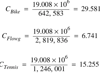
Using Fuwe can now calculate the compression ratios for each of the video sequences. Fc was obtained from Table 4.
Note that the picture density and compression ratio are related by the following formula,
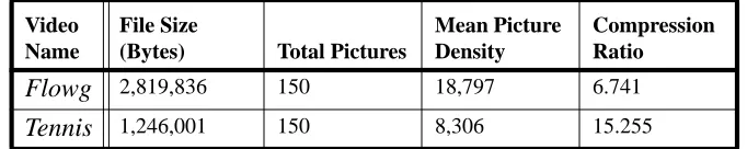
The picture density and compression ratios of the three video sequences was calculated and tabulated in Table 4. Bike had the highest compression ratio of the three video
sequences. It would appear that the motion compensation compression technique used by MPEG was most effective for the type of scene content within Bike. Flowg had the lowest compression ratio of the three video sequences. Obviously, the motion compensation tech-nique did not work as well as it did with Bike. We tried to get a better understanding of the differences in compression ratio by looking at the macroblock type distribution within each picture type
Video Name
File Size
(Bytes) Total Pictures
Mean Picture Density
Compression Ratio
Bike 642,583 150 4,284 29.581
TABLE 4. MPEG video file quantitative information
Fu 150pictures x3x352x240
2 bytes/picture
=
Fu = 150x 126 720( , ) = 19.008x106 bytes
CBike 19.008 10
6 ×
642 583, 29.581
= =
CFlowg 19.008 10
6 ×
2 819 836, , 6.741
= =
CTennis 19.008 10
6 ×
1 246 001, , 15.255
= =
D Fu
N×C
4.3 Macroblock Type Distribution
The distribution of the macroblock type within P and B frames gives an indication of the effectiveness of motion compensation. The more I macroblocks within P and B frames the less effective motion compensation was in finding appropriate motion vectors. I frames will always have the same number of I macroblocks per picture. P frames will have a mix of I and P macroblocks while B frames will have a mix of I, P, B and Bi mac-roblocks. The number of bits per picture depends on the macroblock type selected and the number of bits per macroblock. Macroblock type selection is based on the motion content of the video sequence. For example, when encoding B frames, the encoder attempts to encode the current macroblock as a Bi macroblock. If a Bi macroblock is not appropriate, then the encoder will try to encode it as a P or B macroblock. As a last resort, the encoder will encode the macroblock as an I macroblock. The same strategy is used to encode P frames except the encoder chooses between P and I macroblocks. The more I macrob-locks contained within P and B frames the more bits contained in the picture.
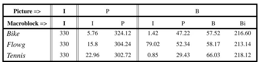
Table 5 shows the mean number of macroblock types per picture type. These Bike had P frames with the lowest mean number of I macroblocks and B frames with the second lowest. One possible reason for this is that for most of the video sequence a small moving object was in the foreground and the background consisted of large surface areas where predictive encoding and interpolation should do well. Flowg had B frames with the high-est mean number of I macroblocks. Flowg consisted of scenery which was panned and contained a multitude of small objects possibly causing mismatches when using predictive or interpolative encoding. Tennis had B frames with the lowest mean number of I mac-roblocks and P frames with the highest mean number of I macmac-roblocks. This would indi-cate that Backward-Prediction worked well, but Forward-Prediction did not when
compared to the other video sequences. It is interesting to note that Flowg had the lowest compression ratio and Bike had the highest. One can infer that the distribution of I mac-roblocks in P and B frames has an affect on compression ratio.
Flowg 2,819,836 150 18,797 6.741
Tennis 1,246,001 150 8,306 15.255
Video Name
File Size
(Bytes) Total Pictures
Mean Picture Density
Compression Ratio
.
4.4 Video Sequence Statistics and Autocorrelation Function
Table 6 shows the cells/slice statistics for the three video sequences. Bike had the highest peak-to-mean ratio which would indicate a proportional relationship between the com-pression ratio and the peak-to-mean ratio. Flowg had the lowest peak-to-mean ratio and the lowest compression ratio. Note that for Bike, Flowg and Tennis sequences the mini-mum cells/slice is one standard deviation away from the mean while the peak multiple standard deviations away. We shall see in the next section that this fact might present a problem for symmetric dynamic bandwidth allocation schemes. AllMux is a time-shifted multiplex of the three video sequences and will be discussed later.
The peak number of cells/slice is determined by the maximum number of cells/slice con-tained within I frames. Referring to Figure 15, we can see that the shapes of the peaks for each of the video sequences is a result of the affect of picture content on the spatial encod-ing of the I frames. Pictures which contain many objects will generate I frames whose macroblocks generate many non-zero AC coefficients. This reduces the effectiveness of the run-length encoding and increases the number of bits per macroblock. For example, the Bike sequence begins with the motorcycle located in the top-half of the picture. The result is an I picture where the largest slices occur at the top of the picture (slices at the top of the picture are located at the left-hand side of the peak). Flowg has flowers covering the bottom half of the picture resulting in the larger slices occurring on the right-hand portion of the peak. We can also see that for this portion of the sequence approximately 90 cells/
Picture => I P B
Macroblock => I I P I P B Bi
Bike 330 5.76 324.12 1.42 47.22 57.52 216.60
Flowg 330 15.8 304.24 79.02 52.34 58.17 213.14
Tennis 330 22.96 302.72 0.85 29.43 66.03 218.12
TABLE 5. Mean number of macroblock types per picture type
Video Name Peak Mean Std. Dev. Variance
Coeff. of Variation
Peak/ Mean
Bike 40 6.4351 7.0445 49.6243 1.0947 6.2159
Flowg 105 26.6080 25.7041 660.6982 .9660 3.9462
Tennis 53 12.0204 13.1238 172.2344 1.0918 4.4092
AllMux 115 44.1887 21.5027 462.3659 .4866 2.6025
slice were required to encode the bottom portion of the picture. Clearly, this is a result of the increased number of non-zero AC coefficients. Tennis has a relatively flat peak. This is due to the fact that the opening scene of this video sequence is a close-up of a bouncing ping-pong ball. Since the ball covers most of the picture, the number of non-zero AC coef-ficients is fairly constant for each slice within the picture.
.The bit-rates can be calculated from the cells/slice data by using the following formula.
This formula simplifies to the following.
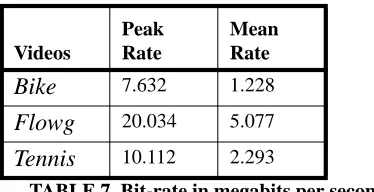
Using this formula we can calculate the peak and mean bit-rates for the video sequences which are shown Table 7. We can see that the bit-rates can vary from 1.228 mbps to 20.034 mbps for these video sequences.
The autocorrelation function for the three video sequences is shown in Figure 16. It is strongly correlated and periodic, decaying with a negative slope with increasing lag. Peaks in the autocorrelation function occur every 45 slices which is due to the occurrence of I and P frames. The peak period is due to the number of B frames there are between I and P frames. This is illustrated more closely in Figure 17. It does appear that the frame
sequence dominates the correlation function rather than the picture content. Livny, et. al. [27] points out that correlated sources can significantly degrade queuing performance. One would have to conclude that these video sequences are highly correlated and would present problems for queueing systems. This raises the question as to whether statistically multiplexing such sources makes sense. We address this issue later on when we discuss time shifted multiplexing.
Videos
Peak Rate
Mean Rate
Bike 7.632 1.228
Flowg 20.034 5.077
Tennis 10.112 2.293
TABLE 7. Bit-rate in megabits per second
B 30pictures
ond
sec
( )x 53bytes
cell
( )x 15 slices
picture
( )x Scells
slice
( )x 8x10⁻⁶ Mb
byte
( )
=
4.5 Statistical Distribution
Early research work indicated that the video picture bit rate had a Normal Gaussian type distribution [13], [17]. While this was true for video conference type sequences containing little motion, recent work shows that the distribution of the number of ATM cells/picture had a Gamma distribution [22], [28] for video sequences with motion and scene changes. Pancha et. al. [9], pointed out that the Gamma distribution fits the cells/slice distribution well for low quality sources (q=16), but did not fit well for higher quality sources (q=4,8). Kishimoto et al. [29] and Heyman et al. [22] pointed out that a more accurate distribution might be a combination of distributions. The former proposed a mix of three Gaussian dis-tributions while the latter proposed a mix of Gamma and Exponential disdis-tributions. Both did not characterize video at the Slice layer. These studies did not include video sequences with B frames and only contained I and P frames.
We attempted to determine if a video sequence, containing B frames, cells/slice distribu-tion would fit the Gamma distribudistribu-tion. The continuous version of the Gamma probability density function (pdf) is given by the following equation:
where is the Gamma function defined by the following integral
The Gamma density function parameters, and , are estimated by using the Method-of-Moments [30]. This method estimates the parameters a pdf by taking the n moments of the data where n is the number of parameters to estimate. In the case of the Gamma Function, there are two parameters to estimate; therefore, two moments are required. The first and second moments of the Gamma function are,
Solving for and we get the following equations:
f x( ) λ λ( )x α−1
Γ( )x e λx
x≥0
( )
= (6)
Γ
( )
x
Γ( )x xα−1e−x
0
∞
∫
dx= (7)
α λ
µ1 = αλ µ2 α
λ2 α2 λ2 + =
α λ
α µ2
v
= λ µ
v
where is the variance is the mean. The Gamma pdf for each of the video sequences was generated using the estimated values for and shown in Table 8.Note that as approaches 1, the Gamma pdf simplifies to an Exponential distribution shown in (8).
Figure 18 shows the histograms for the cells/slice distribution for Bike, Flowg and Tennis. The x and y axis are normalized for comparative purposes. Note that all of the video sequences have a distinctive exponential shape. The estimated Gamma pdf is overlaid onto the histogram plot. There are significant gaps which exist where the Gamma pdf overestimates the number of cells/slice between the x-axis values 0.2 to 0.4. This would indicate that these video sequences will not fit the Gamma distribution. We confirm this by using the QQ plot technique.
The QQ plot [31] is used to determine if two sets of data have the same distribution. This method involves taking the cumulative distribution function (cdf) of both sets of data and comparing their x-axis values for a given y-axis value. This is illustrated in Figure 8. The x1 and x2 values are plotted with x1 values on the x-axis and x2 values on the y-axis. The values x1 and x2 are referred to as the quantiles. If the two sets of data have the same dis-tribution, then the QQ plot will show the (x1,x2) points forming a straight line.
We can see from the QQ plots in Figure 20 that while Bike fit the Gamma distribution well both Flowg and Tennis did not. It is interesting that Bike had the highest compression ratio, but cannot claim there is a correlation between compression ratio and the Gamma tion without study further video samples. It does appear; however, that a single distribu-tion will not fit VBR video containing I/B/P frames.
Video Sequence
Bike 0.8345 0.1297
Flowg 1.0716 0.0403
Tennis 0.8389 0.0698
AllMux 4.0988 0.0910
TABLE 8. Gamma pdf parameters.
v µ
α λ α
f x( ) = λe−λx (x≥0) (8)
5.0 Impact on Dynamic Bandwidth Allocation Schemes
Referring to Figure 15, we can see that sequences which include B frames produce dis-tinctive peaks-and-valleys in the cells/slice plot. The peaks are caused by I and P frames and the valleys by B frames. The peaks are 15 slices wide and the valleys are 30 slices. There is an abrupt increase in the number of cells/slice when the sequence goes from B frames to I or P frames. This behavior makes it difficult for a traffic predictor to determine when to request additional bandwidth if only the raw video bit stream is monitored. If the traffic predictor monitors the number of cells per frame of all I/B/P frames, it could falsely predict that more bandwidth is required.
In Pancha, et al [9] a simple method, shown in (9),was used to predict whether extra band-width was required.
The estimator represents the number of cells for frame n given cells occurred in frame n-1. The value is the threshold and was set to one standard deviation. The
assumption was that the probability that the number of cells per frame exceeded one stan-dard video between frames was very small. While this is true for video conference type sequences containing only I/P frames, Figure 15 clearly shows this is not the case with I/
x1 x2
y
Data 1
Data 2
FIGURE 8. Illustration of generating QQ plot coordinates
cn = max(µ,cn−1+∆) (9)
cn cn−1
B/P frame sequences. As a consequence, the traffic predictor must be selective in the frames it chooses to monitor. We propose that monitoring I frames or slices within I frames would be sufficient for traffic prediction since I frames contain the largest number of cells and provide a strong indication of significant spatial content changes. We can see from Figure 14 that if the three video sequences were concatenated, there would be dis-tinct changes in the I frame peak cells/slices between Bike, Flowg and Tennis. An alloca-tion of 6.678 mbps would be sufficient for Bike, 19.08 mbps for Flowg and 9.540 mbps for
Tennis.
6.0 Time-Shifted Multiplexing of the Video Sequences
When looking at the cells/slice data shown in Figure 15 one cannot help but notice the dis-tinct peaks and valleys generated by an I/B/P stream. This causes the autocorrelation func-tion to not only be strongly correlated, but periodic as well. This characteristic appears to be consistent amongst the three video sequences. This characteristic would appear to cause problems when multiplexing multiple VBR streams with I/B/P frames. Since the streams are periodic and not statistical in terms of arrivals, if the streams are multiplexed improperly significant inefficiencies in bandwidth utilization might occur. An example would be if we multiplexed the three video streams where I frames overlapped. Since each sequence has the same I/B/P frame pattern, I frames will always overlap for the duration of playback. For this reason, we look at a way to multiplex VBR I/B/P video streams which attempts to take advantage of this periodic behavior. We called this method Time
Shifted Multiplex or TSM.
We looked at what the effect of multiplexing the three video sequences would have on the resultant cells/slice statistics. We generated the sequence called AllMux which is a TSM of the three video sequences. This sequence is generated by shifting the cells/slice data so that I or P frames from one sequence would overlap B frames from another sequence. Each of the sequences were contained in a vector consisting of the number of cells/slices.
Bike was not shifted. Flowg was shifted forward in time by 15 slices and Tennis by 30
slices. The resultant vectors were added together and the first 30 slices were truncated to form the new AllMux vector. The first two pictures were discarded since they were adja-cent I and P frames which occur only during the beginning of playback.
peaks and valleys shown for the non-multiplexed sequences. Also, the distribution tends to be more Gamma-like than Exponential. The QQ plot confirms this by showing quantile points which tend to fall form a straight line.
The drawback to this approach is that video streams would need to be delayed by the video server in order to insure proper overlap of frames. This can cause problems where frames are not delivered to the client in time for playback, thereby causing frame slips. It might be possible; however, to delay frames given certain delay constraints which will avoid this problem. Also, if a video server has might have some control as to when to start playback of multiple video streams and offset them in order to overlap properly. These issues require further investigation and study. In essence, it does appear that statistically multiplexing VBR video with I/B/P frames does not make sense.
7.0 Video Model Using Markov Chain
We used an 8-state discrete-time, discrete-state Markov Chain as a model for the three video sequences and the multiplexed sequence. We attempt to see if the pdf generated by the Markov Chain produces a better fit for the cells/slice distribution. The number of states was selected based on the ratio of the peak cells/slice and the standard deviation. For example, Bike had a peak of 40 cells/slice and a standard deviation of 7.0445 cells/slice. This gives a ratio of 5.68:1 which we approximated to 6:1 which would mean using a 6 state Markov Chain; however, we chose 8 states for more accuracy.
Each state represents a range of the number of cells/slice. The range was calculated by tak-ing the peak number of cells/slice and dividtak-ing it by 8. So for Bike the range of cells/slice is 40/8 or 5 cells/slice. The ranges shown in Table 9 define the discrete-state of the
Markov Chain. For example, if the number of cells/slice in the Flowg video is 60, the Markov Chain would be in state 4. We used the same number of states for all of the video sequences so that we could compare their steady-state distributions.
and 80 transitions for Bike, Flowg and Tennis respectively. We calculated the steady-state probabilities by multiplying the matrix n times until all the column transition probabilities were the same. In Figure 22, we compared the steady-state probabilities to the histogram data. We can see that the pdf produced by the Markov Chain is a better fit than the Gamma pdf. Specifically, the gap which existed between x-axis values 0.2 and 0.4 is much less pronounced.
Markov Chain
State Bike Flowg Tennis AllMux
0 0-5 0-14 0-7 0-15
1 6-10 15-28 8-15 16-30
2 11-15 29-42 16-22 31-45
3 16-20 43-56 23-29 46-60
4 21-25 57-70 30-36 61-75
5 26-30 71-84 37-42 76-90
6 31-35 85-98 43-49 91-105
7 36-40 99-112 50-57 106-120
TABLE 9. Markov Chain cells/slice ranges.
0.9143 0.0564 0.0160 0.0056 0.0028 0.0021 0.0021 0.0007 0.2428 0.5405 0.1358 0.0462 0.0116 0.0116 0.0087… 0.0029 0.0510 0.3214 0.4082 0.1480 0.0561 0.0051 0.0102 0 0.0915 0.0423 0.3028 0.3944 0.1197 0.0493 0 0 0.1667 0.0500 0.0667 0.3833 0.2000 0.1167 0.1067 0 0.1463 0.1220 0 0.1707 0.2927 0.1951 0.0488 0.0244
0 0.0400 0 0.0400 0 0.4400 0.4800 0
0 0 0 0.5000 0 0 0.5000 0
i
j
Bike