Structure-based software reliability prediction*

In Proc. of Advanced Computing (ADCOMP) '97, Chennai, India

Structure-Based Software Reliability Prediction

Swapna S. Gokhale and Kishor S. Trivedi

Center for Advanced Computing and Communication

Dept. of Electrical and Computer Engineering

Box 90291, Duke University, Durham, NC 27708-0291

Abstract

Prevalent approaches to software reliability model-ing are black-box based, i.e., the the software system is considered as a whole and only its interactions with the outside world are modeled without looking into its in-ternal structure. However, with the advancement and widespread use of object oriented systems design and development, the use of component-based software de-velopment is on the rise. Software systems are devel-oped in a heterogeneous (multiple teams in dierent en-vironments) fashion, and hence it may be inappropriate to model the overall failure process of such systems us-ing only one of the several software reliability growth models. In this paper we outline the constituents of the structural models. We then present a exhaustive anal-yses of the classes of methods where the architecture of the application is modeled either as a discrete time Markov chain (DTMC) or a continuous time Markov chain (CTMC), and illustrate these methods using ex-amples.

1 Introduction

The impact of software structure on its reliability and correctness has been highlighted as early as 1975 by Parnas 4]. Prevalent approaches to software relia-bility modeling however are black-box based, i.e., the software system is considered as a whole and only its interactions with the outside world are modeled, with-out looking into its internal structure. With the ad-vancement and widespread use of object oriented sys-tems design and development, the use of component-based software development is on the rise. The soft-ware components can be commercially available o the shelf (COTS), developed in-house, or developed con-tractually. Thus, the whole application is developed

Supported by a contract from Charles Stark Draper Labo-ratory and in part by Bellcore as a core project in the Center for Advanced Computing and Communication

in a heterogeneous (multiple teams in dierent envi-ronments) fashion, and hence it may be inappropriate to model the overall failure process of such applications using only one of the several software reliability growth models (black-box approach). Predicting reliability of such heterogeneous application taking into account the information about its architecture, testing and reliabil-ities of its components, is thus absolutely essential.

In this paper, we outline the constituents of the structural models for the prediction of software reliabil-ity. We characterize the structural approaches to relia-bility prediction, based on the models used to dene the architecture of the software, failure behavior of its com-ponents and that of the interfaces between them, and the method of analyses they employ. We then present an exhaustive analyses of the classes of methods where the architecture of the application is modeled either as a discrete time Markov chain (DTMC) or a continu-ous time Markov chain (CTMC), and illustrate these methods using examples.

The layout of the paper is as follows: Section 2 dis-cusses the constituents of the structural models, Sec-tion 3 gives a brief overview of discrete and continuous time Markov chains, Section 4 describes various DTMC and CTMC techniques for reliability prediction, Sec-tion 5 illustrates the techniques presented in SecSec-tion 4 with various examples, and Section 6 presents conclu-sions and directions for future research.

2 Constituents of Structural Models

The constituents of structural models include:

Architecture of the software: This is the

rected Acyclic Graph). DTMC, CTMC, and SMP can be further classied into irreducible and absorb-ing categories, where the former represents an innitely running application, and the latter a terminating one. DAG models concurrent software having no loops and can be used to predict time to completion of a con-current program 5]. Transitions among modules could either be instantaneous or there could be an overhead in terms of time.

Failure behavior: The failure behavior of the

modules and that of the interfaces between the mod-ules, can be specied in terms of the probability of failure (or reliability), or failure rate (constant= time-dependent). The time-dependent failure rate could be the failure rate associated with one of the reliability growth models 2].

The architecture of the software can be combined with the failure behavior of the modules and the inter-faces into a composite model which can then be ana-lyzed to predict reliability of the software. The com-posite model also enables the computation of various performance measures such as the time to completion of the application. We will refer to this method of re-liability prediction as the \Composite Method". The other possibility is to solve the architectural model and superimpose the failure behavior of the modules and that of the interfaces on to the solution, to predict reliability. We refer to this method as \Hierarchical Method".

We characterize every approach by a tuple (MethodModelModules=InterfacesTrans:),

where Method indicates the method

of analysis, Model indicates the architectural model, Modules=Interfacesindicates the failure behavior of the modules=interfaces,Trans:indicates the nature of transitions (timed=instantaneous).

3 Overview of Markov Models

In this section we provide an overview of discrete time Markov chains (DTMCs) and continuous time Markov chains. The interested reader is referred to 5, 6] for a detailed study of these topics.

Let X(t) denote a discrete state stochastic pro-cess. Without loss of generality, we assume the dis-crete state space I 2 f012:::g. Let P(X(t) = j)

denote the probability that the process is in state j at time t. X(t) is a Markov chain i, for any or-dered times t0 < t1 < t2::: < tn < t, the conditional

probability mass function of X(t) for given values of X(t0)X(t1):::X(tn), depends only on X(tn).

Time-dependent state probabilities of the Markov

chain at timetare dened by the vector:

(t) = 0(t)1(t):::] (1)

wherej(t) =P(X(t) =j). The objective of the

anal-ysis of a Markov chain is to obtain these state proba-bilities at specic values of t, and in the steady state (t=1).

For our purposes, Markov chains can be classied into the following two categories:

Irreducible: A Markov chain is said to be

irre-ducible if every state can be reached from every other state.

Absorbing: A Markov chain is said to be

absorb-ing, if there is at least one statei, from which there is no outgoing transition. A Markov chain upon reaching an absorbing state is destined to remain there forever.

Depending upon the points in time when the tran-sitions can take place, Markov chains can be classied as discrete time or continuous time as discussed in the subsequent subsections.

3.1 Discrete Time Markov Chains

In case of a discrete time Markov chain (DTMC), the points at which the state changes occur are discrete, and without loss of generality we let the parameter space T 2 f012:::g.Let P = p

ij] be the one-step

transition probability matrix. Pis a stochastic matrix

since all the elements in a row of P sum to one, and

each element lies in the range 01].

The state probability vector at time stepndenoted by (n) in terms of the initial probabilities (0), is given by 6]:

(n) =(0)P(n) (2)

The matrix P(n) in Equation (2) is called the n

-step transition probability matrix of the DTMC. Let pij(n), denote the (ij)-th entry of the matrix

P(n).

pij(n) denotes the probability of reaching state j at

time step n, starting from state i. For steady state analysis of a nite, irreducible and aperiodic DTMC, we take limits on both sides of Equation (2). This gives us the following system of equations for computing the probability vector in the steady state:

=:P :e= 1 (3)

where e = (11:::1) T

and the subscript T denotes the transpose.

In the case of a DTMC with one or more absorbing states, the expected number of times the application visits statej, denoted byVj, can be computed by

solv-ing the followsolv-ing system of linear equations: Vj=

X

Vipij+j(0) (4)

3.2 Continuous Time Markov Chains

The analysis of the continuous time or continuous parameter Markov chains is similar to the discrete pa-rameter case, except that the transitions can occur at any instant of time.

Let the innitesimal generator matrix Q = q ij] of

the CTMC be dened so that qij is the rate of

transi-tion from stateito statej, and: qii =

; X

i6=j

qij (5)

The state probability vector(t) for a CTMC obeys

the Kolmogorov dierential equation: d(t)

dt =(t)Q (6)

For steady state analysis, taking limits of both sides of Equation (6), we have the following system of equa-tions:

:Q= 0 :e= 1 (7)

The (ij)-th entry of the matrixQdenoted byq ij is

the rate at which the system goes from stateito state j, and ;q

ii is the rate at which the system departs

from statei.

The average amount of time spent by the CTMC in state i during the interval (0t), denoted by Li(t) is

given by:

Li(t) = Z

t

0

i(x)dx (8)

Integrating both sides of Equation (6), we obtain a dierential equation for the vectorL(t):

dL(t)

dt =L(t)Q+(0) (9)

For a CTMC with one or more absorbing states, Equation (9) becomes:

Q=(0) (10)

where

lim

t!1

L(t) = (11)

whereirepresents the expected time spent in module

i, until absorption.

4 ReliabilityPrediction

In this section, we discuss various approaches to reli-ability prediction when the architecture of the applica-tion is modeled either by a DTMC or a CTMC. Some of these approaches have been presented in the litera-ture, and are discussed here for the sake of complete-ness, and to highlight their merits and demerits in the light of the exhaustive analysis presented here. Each method will be identied by the tuple in Section 2. We assume a single entry and exit state for a terminating application.

4.1 DTMC Based Approaches

DTMC 1:(CompositeA;DTMCR=11)

This method has been discussed by Cheung 1]. The ar-chitecture of the model consists of the transition prob-ability matrixW =wij, which is the probability that

the transition (ij) is taken when the control is at node i. The reliability of nodeiis assumed to beRi. Let the

entry node be denoted by 1, which is the initial state of the DTMC. The terminal statesCandF are added, which represent the state of correct output and failure respectively. For every nodei, a directed branch (iF) is created with transition probability (1;R

i),

repre-senting the occurrence of an error in the execution of modulei. The original transition probability betweeni andjis modied toRiwij, which represents the

trans-fer of control toj from i, conditional to the successful execution of i. Thus pij =Riwij. A directed branch

is created from the exit node n to C, with transition probability Rn, which represents the correct

termina-tion at the exit node. Note thatwij = 0 if the branch

(ij) does not exist. The reliability of the application afterksteps, is the probability of reaching the terminal state C, starting from the initial state 1 and is given by p1C(k). The reliability of the application (without

qualication) is given by 1 X

k =0

p1C(k).

DTMC 2: (CompositeI;DTMCR=11)

The composite model of an irreducible DTMC repre-senting an innitely running application along with the reliabilities of the components, is constructed by adding a terminal state F which corresponds to the failure of the application. We can compute the mean time to failure of the application in this case.

DTMC 3: (HierarchicalA;DTMCR=11)

The reliability of the application when the architecture is represented by an absorbing DTMC and the reliabil-ities of the components are known, using hierarchical method of analyses is given by:

R=n;1 Y

i=1

Ri ViR

n (12)

whereRiandVidenote the reliability and the expected

number of visits to moduleirespectively. Ifti denotes

the expected time spent in moduleiper visit, then the expected execution time t of the application is given by 6]:

t=n;1

X

i=1

Viti+tn (13)

DTMC 4: (HierarchicalA;DTMCCFR=11)

is modeled by an absorbing DTMC and a constant fail-ure rate is associated with each of the components is:

R= n Y

i=1

e; i

t

i V

i (14)

whereVidenotes the expected number of visits to

com-ponenti, and ti is the expected time spent in

compo-nentiper visit.

DTMC 5: (HierarchicalA;DTMCTDR=11)

When a time dependent failure rate is associated with each module, and the architecture of the application is modeled by an absorbing DTMC, its reliability is given by:

R= n Y

i=1

e; R

V

i t

i

0

i()d

(15) where Vi andti are as dened before. Viti is thus the

expected total time spent in moduleiper execution of the application.

DTMC 6: (HierarchicalI;DTMCR=11)

The reliability of an application when the architecture is dened by an irreducible DTMC and the reliabilities of the components are known, is given by:

R= n X

i=1

iRi (16)

wherei is the probability that the application is

exe-cuting module i, in the steady state.

DTMC 7: (HierarchicalI;DTMCCFR=11)

The overall failure rate and the reliability of the appli-cation denoted by and R(t) respectively, when the architecture of the application is modeled by an irre-ducible DTMC, and a constant failure rate is associated with its components is given by:

= n

X

i=1

ii R(t) =e

; t (17)

4.2 CTMC Based Approaches

CTMC 1: (CompositeA;CTMCCFR=11)

The architecture of the software is described by a CTMC, by specifying a distribution for the execu-tion time for each module, and intermodular transiexecu-tion probabilities. The terminal statesC andF which rep-resent successful and abnormal termination of the ap-plication respectively, are added, and the innitesimal generator matrix Q

c corresponding to this composite

model is constructed in the following manner: For ev-ery nodei, a directed branch (ij) is created with rate iwij, where the distribution of the execution time of

modulei, is given byexp(i), andwij is the

probabil-ity that the control is transferred to modulejafter the successful execution of modulei. Thusqij =iwij. An

additional directed branch is created from every nodei to nodeF, with a transition ratei, corresponding to

the failure of node i. A branch is added from node n to C with raten corresponding to the successful

ex-ecution of the application. The composite model can then be solved to compute the probability of being in state C, corresponding to the successful execution of the application. The distribution of the time to com-pletion of the application can also be obtained in this case. F(t) denotes the probability of failure at time

t, F(

1) denotes the eventual probability of failure,

while C(t) denotes the probability of successful

exe-cution of the application by time t.

CTMC 2: (CompositeI;CTMCCFR=11)

The innitesimal generator matrix in this case, is also constructed by adding a state F corresponding to the failure of the application. The addition of this state transforms the irreducible CTMC into an absorbing one, with a single absorbing state. Given innite time, the application will reach this absorbing state with probability 1. The mean time to failure (MTTF) of the application is given by:

MTTF = n

X

i=1

i (18)

where i are as dened in Equation (11).

CTMC 3: (HierarchicalA;CTMCR=11)

When the architecture of the application is represented by an absorbing CTMC, and the reliabilities of the components are known, the reliability of the applica-tion using hierarchical analyses is given by Equaapplica-tion (12). The visit counts are computed by the analysis of the embedded DTMC.

CTMC 4: (HierarchicalA;CTMCCFR=11)

The reliability of the application with an architecture represented by an absorbing CTMC, and the compo-nents fail as per a constant failure rate is:

R(t) = n Y

i=1

e; i

L

i

(t) (19)

whereiis the failure rate of modulei, andLi(t) is the

expected time the application spends executing mod-ulei during a single run as per Equation (9).

CTMC 5: (HierarchicalA;CTMCTDR=11)

by:

R(t) = n Y

i=1

e; R

L

i (t)

0 i

()d

(20) where i() denotes the failure intensity of modulei,

and Li(t) denotes the expected time spent in module

i, as given by Equation (9).

CTMC 6:(HierarchicalI;CTMCR=11)

The analyses in this case is similar to that of its DTMC counterpart, and the reliability of the application is given by Equation (16). This approach has been dis-cussed by Laprie and Kanoun 3].

CTMC 7:(HierarchicalI;CTMCCFR=11)

The analysis here is also similar to the corresponding DTMC case, and has been discussed by Laprie and Ka-noun 3]. We assume that the failure rates are small as compared to the rates governing the transitions among the components, equivalently stated a large number of transitions will take place among the components, be-fore the occurrence of a failure. The overall failure rate and the reliability of the application are given by Equation (17).

Thus we see that composite methods of analyses are convenient, if the type of the model used to represent the architecture of the application is retained, after combining it with the failure behavior of the compo-nents. For instance, composite analysis is possible if the architecture is modeled by a DTMC, and the reli-abilities of the components are given, since the combi-nation of this information results in a DTMC model. Similarly, in case of a CTMC-based architecture, com-posite analysis is possible if the failure of the compo-nents is characterized by constant failure rates. Hier-archical analyses is possible in case of all the applica-tions when the architecture is described by absorbing DTMC=CTMC, irrespective of how the failure behav-ior of the components is characterized. In the irre-ducible case, hierarchical analyses can be used to pre-dict reliability, when the components are characterized either by their reliabilities or constant failure rates. Ex-tensions to this basic scheme are under investigation.

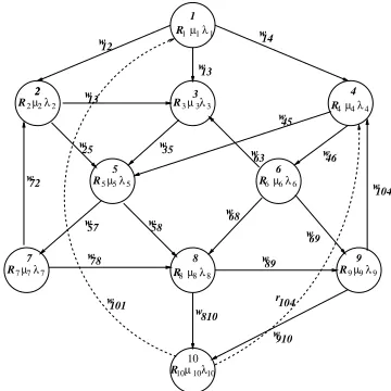
5 Illustrations

In this section, we illustrate the various methods dis-cussed in the previous section with examples. The ba-sic application used for this purpose has been described in 1], which is an absorbing DTMC, and the reliabil-ities of the modules are given. This basic example is subsequently modied=updated to describe various ar-chitectures and failure behaviors. The application

un-R1µ λ1 1

R2µ λ2 2 R3 3µ λ3 R4µ λ4 4

R5µ λ5 5 R6µ λ6 6

R7µ λ7 7 R8µ λ8 8 R9µ λ9 9

µ λ10

R10 10

1

2 3 4

5 6

7 8 9

2

10

12 14

13 13

25 35

72

57

78 58

68

89

r 69 63 46

45

101

810

104

910

104 w

w

w w

w

w

w

w w w

w w w

w

w

w w

w w w

Figure 1. Example of a Program Control Flow Graph

der consideration has 10 modules where 1 represents the entry state and 10 represents the exit state. The reliabilities of the modules are given in Table 2, and the intermodular transition probabilities are given in Table 1.

Table 1. Intermodular Transition Probabilities

p(12)=0:60 p(13)=0:20 p(14)=0:20

p(23)=0:70 p(25)=0:30

p(35)=1:0

p(45)0:40 p(46)=0:60

p(57)=0:40 p(58)=0:60

p(63)=0:30 p(67)=0:30 p(68)=0:10 p(69)=0:30

p(72)=0:50 p(79)=0:50

p(84)=0:25 p(810)=0:75

p(98)=0:10 p(910)=0:90

Table 2.Ri=i=i of the components

Mo dule# Reliability(R

i

) CFR(

i

) TTC(

i )

1 0:99 0:001 0:1

2 0:980 0:002 0:2

3 0:990 0:0015 0:15

4 0:970 0:0005 0:05

5 0:950 0:00075 0:075

6 0:995 0:0025 0:25

7 0:995 0:00175 0:175

8 0:950 0:00025 0:125

9 0:975 0:00225 0:225

10 0:985 0:00025 0:025

is 0:8351, while using the hierarchical method as per DTMC 3 is 0.8188. Assuming that the average time spent in a module per visit in a single execution of the application is 0:03, the reliability of the applica-tion as perDTMC 4 is 0:8177. Without loss of gener-ality, we assume that the time-dependent failure rate associated with each component is that of the Goel-Okumoto model 2], and is 0:34 0:0057 e;0:0057t.

The reliability of the application in this case is given by 0:99. The rst modication we consider is a trans-formation of the architecture from an absorbing DTMC to an irreducible DTMC, which we achieve by adding two directed branches w101 = 0:8, and w104 = 0:2.

These two transitions are shown by dashed lines in the control ow graph in Figure 1. The reliability of the application as perDTMC 6 is 0:97519. The com-posite model has a single absorbing state correspond-ing to the failure of the application, and the steady state probability of reaching that state is 1. How-ever, we can compute mean time to failure (MTTF), according to DTMC 2, which is 55:551. We next as-sume that the failure behavior of the modules is given by a constant failure rate as in Table 2. The over-all failure rate of the application is given by 0:0011, the reliability as per DTMC 5, is R(t) = e;0:0011t,

and hence the MTTF = 1

0:0011 = 909:09. The

ab-sorbing DTMC is then transformed to an abab-sorbing CTMC, by associating a exponentially distributed ex-ecution time for each module, as given in Table 2. The reliability of the application as per CTMC 3 is 0:8148, as per CTMC 1 is 0:92664, as per CTMC 4 is 0:9407, and as per CTMC5 is 0:8858. The ab-sorbing CTMC is then transformed to an irreducible CTMC by adding the same two transitions as before. The reliability of the application as per CTMC 6 is 0:97578. The overall failure rate of the application as per CTMC 7 is 0:00086320, and the reliability is given by R(t) = e;0:00086320, and hence the MTTF

is 1

0:00086320 = 1158. The mean time to failure of the

application as per (CTMC2) and is 1150. Whenever both hierarchical and composite methods of analyses are feasible, the dierence in the reliability predictions obtained using these two methods can be attributed to the fact that the hierarchical method provides an ap-proximation to the reliability estimates obtained using the composite method.

6 Conclusions and Future Research

In this paper we have discussed the specication and solution techniques for the structural models to quan-tify software reliability. In addition, we have also pro-posed a classication of the techniques based on the

models used to dene the architecture of the appli-cation, failure behavior of the components, and the method of analyses. We have presented an exhaus-tive discussion of the discrete time and continuous time Markov chain based methods. We have illustrated the techniques with examples. Empirical validation of the methods discussed here is being carried out.

References

1] R. C. Cheung. \A User-Oriented Software Reliabil-ity Model". IEEE Trans. on Software Engineering, SE-6(2):118{125, March 1980.

2] W. Farr. Handbook of Software Reliability Engi-neering, M. R. Lyu, Editor, chapter Software Re-liability Modeling Survey, pages 71{117. McGraw-Hill, New York, NY, 1996.

3] J. C. Laprie and K. Kanoun. Handbook of Software Reliability Engineering, M. R. Lyu, Editor, chapter Software Reliability and System Reliability, pages 27{69. McGraw-Hill, New York, NY, 1996. 4] D. L. Parnas. \The Inuence of Software Structure

on Reliability". In Proc. 1975 Int'l Conf. Reliable Software, pages 358{362, Los Angeles, CA, April 1975.

5] R. A. Sahner, K. S. Trivedi, and A. Puliato. Performance and Reliability Analysis of Computer Systems: An Example-Based Approach Using the SHARPE Software Package. Kluwer Academic Publishers, Boston, 1996.