How informative is Wright's estimator of the number of genes affecting a quantitative character?

Copyright 0 1990 by the Genetics Society of America

How

Informative Is Wright’s Estimator of the Number of Genes Affecting a

Quantitative Character?

Zhao-Bang Zeng, David Houle and C. Clark Cockerham

Department of Statistics, North Carolina State University, Raleigh, North Carolina 27695-8203 Manuscript received February 24, 1990

Accepted for publication May 24, 1990

ABSTRACT

S. Wright suggested an estimator, i , of the number of loci, m, contributing to the difference in a quantitative character between two differentiated populations, which is calculated from the phenotypic means and variances in the two parental populations and their FI and F2 hybrids. T h e same method can also be used to estimate m contributing to the genetic variance within a single population, by using divergent selection to create differentiated lines from the base population. In this paper we systematically examine the utility and problems of this technique under the influences of unequal allelic effects and initial allele frequencies, and linkage, which are known to lead i to underestimate m. In addition, we examine the effects of population size and selection intensity during the generations of selection. During selection, the estimator i rapidly approaches its expected value at the selection limit. With reasonable assumptions about unequal allelic effects and initial allele frequencies, the expected value of i without linkage is likely to be on the order of one-third of the number of genes. T h e estimates suffer most seriously from linkage. T h e practical maximum expectation of i is just about the number of chromosomes, considerably less than the “recombination index” which has been assumed to be the upper limit. T h e estimates are also associated with large sampling variances. An estimator of the variance of i derived by R. Lande substantially underestimates the actual variance. Modifications to the method can ameliorate some of the problems. These include using F3 or later generation variances or the genetic variance in the base population, and replicating the experiments and estimation procedure. However, even in the best of circumstances, information from TG is very limited and canbe misleading.

T

he number of genes that contribute variance in

a quantitative character has important implica- tions for evolution and for plant and animal breeding. T h e simplest and least expensive methods for estimat- ing this number involve observing the means and variances of differentiated populations and their hy- brids. Several statistical methods for estimating the “effective” or “minimum” number of loci segregating

have been proposed (e.g., CASTLE 192 1; STUDENT

1934; PANSE 1940; PARK 1977a; JINKS and TOWEY

1976; COMSTOCK and ENFIELD 1981). T h e original

method of WRIGHT (in CASTLE 1921), as elaborated

by WRIGHT (1968), is the simplest and most widely

used method. WRIGHT’S method relates the difference

in the means of two inbred lines to the variance of their F2 and backcross populations. LANDE (198 1)

pointed out that WRIGHT’S method could also be used

with outbred populations. He suggested that the same method could be applied to artificially selected lines (high and low) from a single base population.

Since one of the main assumptions of WRIGHT’S method is that one parent contains all the increasing

alleles and the other parent contains all the decreasing

alleles, the use of selected lines directed at making this assumption true is very appealing. Other assump-

tions in WRIGHT’S method are additive gene action,

Genetics 1 2 6 235-247 (September, 1990)

unlinked loci, and equal allelic effects at all loci. Many authors have addressed the effects of relaxing each of these assumptions in turn (SHULL 1921; WRIGHT

1968; FALCONER 1981; LANDE 1981; MATHER and

JINKS 1982). T h e relaxation of several of these as-

sumptions simultaneously has not been explored. Nevertheless, it has long been clear that when these

assumptions are violated the method substantially

underestimates the true number of loci.

When lines are created by selection it is tempting to assume that the assumption of fixation of increasing alleles in high lines and decreasing alleles in low lines is assured. However, in the small populations of typical

artificial selection experiments, genetic drift may have

an important effect on fixation probability for loci of small effects. In addition, departures from the other assumptions have an impact on the process of fixation, beyond their impact on the estimation process. In this

paper we explore the utility of selection lines for

estimating the minimum number of loci as a function of linkage and the distributions of allelic effects and frequencies in the base population. We will, however, keep the assumption of additive allelic effects.

An additional issue is the sampling variance of the

estimation process. LANDE (1 98 1) derived an approx-

effective number of loci, and pointed out the need for modest sample sizes during estimation. We report here simulations which emphasize the magnitude of sampling variance.

When all of these factors are considered simulta- neously it is clear that WRIGHT'S method is more apt to be misleading than illuminating.

WRIGHT'S METHOD

WRIGHT'S method involves the means, Ph and P I ,

and variances, u i and a:, of the parents from the high

and low populations, respectively, and the variance

uEp, of their F2. T h e estimate, i , of the number of loci is given by

where u: = uE2

-

( u i

+

u : ) / 2 [see LANDE ( 1 9 8 1 ) and

WRIGHT ( 1 9 6 8 ) for details]. There are other methods

of determining

cr:

including the use of backcrosses

and FI (COCKERHAM 1 9 8 6 ) but all provide the same

theoretical value in our context.

Equation 1 would give the number of loci, m , by

expectation, if the four assumptions mentioned in the

introduction hold. Deviations from the assumptions

will usually cause an underestimate of the number of

loci, so WRIGHT'S method is usually said to estimate

the effective or minimum number of loci.

DIVERGENT SELECTION

Consider a base population in which m loci each

with two alleles are segregating. Alleles are additive within and between loci. For the ith locus the geno- typic effects and frequencies in the population are given as

Genotype AiAi Aiai U ~ U ,

Initial Frequency

_p'

_{2p,q, q'}

Effects ai

4 2

0

We assume that a, and

p i

are independent and are

distributed among loci with density function f ( a ) ,

0

<

a

<

03, and Pr(f), respectively.

We consider continuous truncation selection for

high and low values of the quantitative character from the base population. Mutation is ignored.

Estimation from the fixed selection lines (at selection limit)

Let us first consider the selection limit without

linkage. Let uih and vil be the indicator variables for

the ith locus with the properties that

1 if the allele Ai

0 otherwise

is fixed in the high line

and

1 if the allele Ai

0 otherwise.

Ull = is fixed in the low line

Then we have 8 ( V i h ) = 8 ( v , ? h ) = uih and 8 ( v i l ) =

8 ( u : ) = u,l, where u i h and u,l are the probabilities of

the allele Ai being fixed in the high and low lines,

respectively, at the selection limit, and 8 denotes

expectation. T h e difference between the means of the high and low lines, aside from experimental error, is

P h

-

Pl = (vlh

-

V i l ) &

( 2 )

where the summation is taken over all loci. Both

parental and F1 populations have no genetic variance

and the genetic variance in the F2 is

U: = (Vih

+

Vil

-

%ihUil)U?/8 (3)

because the chance of F1 individuals being heterozy- gous for the ith locus is vih(1

-

u,l)

+

vil(1

-

V i h ) and

the allele frequency is $4 for all loci segregating in the

FB. The expected value of i in this context is then

This expectation is difficult to analyze in general. However, the ratio of expectations

is easier to analyze, and it has the property that

8 ( i ) 5 &

<

a(m)

+

1

when the allelic effects and initial frequencies are

constant among loci (see APPENDIX). As selection in-

creases, & converges to 8(6). This suggests that & is

a good approximation of 8 ( i ) . Assuming that the

fixation status of one locus is independent of that at

other loci, and that allelic effects as well as initial

frequencies are independent among loci,

after taking the expectation with respect to v .

In this paper we would like to express results as the proportion of loci detected, i.e., 8 ( i ) / m or & / m . In-

stead of analyzing 8 ( i ) / m , we will, however, define

the proportion of loci detected as

which ranges from 0 to 1 . T h e above analysis indicates

that

Wright's Estimator of Gene Numbers 237

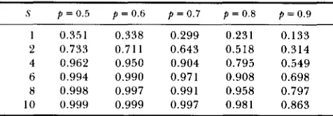
TABLE 1

Expected proportion, Z, of the loci detected for various values

of S(= Nsa) and p from Equation 8

S p = 0.5 p = 0.6 p = 0.7 p = 0.8 p = 0.9

1 0.351 0.338 0.299 0.231 0.133

2 0.733 0.711 0.643 0.518 0.314

4 0.962 0.950 0.904 0.795 0.549

6 0.994 0.990 0.971 0.908 0.698

8 0.998 0.997 0.991 0.958 0.797

10 0.999 0.999 0.997 0.981 0.863

for equal allelic effects and initial frequencies. Our

simulations, shown in Table 2 , suggest that this ine-

quality also holds when these assumptions are relaxed.

T h e difference between

Z

and h/m is at most llm.

T h e next step is to evaluate

Z.

T h e fixation proba-

bilities in the high and low lines are given, by the diffusion approximation, as

1

-

e-2NsaP

u h = 1

-

e - 2 N s a

and

1

-

e2NsaP u1 =

1

-

e 2 N s a

(KIMURA 1957), where N is the effective population

size, s = l/a, L is the standardized selection differential,

and u is the phenotypic standard deviation in the base

population. When a and

p

are constant among loci, it

is easy to show that

e - 2 N ~ a p + e - 2 N s a ( I - p )

z = 1 -

1 + e - 2 N s ~ (8)

which increases as Nsa increases and decreases as

p

deviates from 0.5 (see Table 1 ) .

Effects of variation of allelic effects: Variation of

a among loci is expected to decrease the proportion

of loci detected. But the distribution of a is generally

unknown. To analyze the effect of inequality of allelic

effects among loci on

Z,

we assume that a is distributed

among loci with the gamma distribution

p P , P - 1

f(.)

= O S a < a c ,

o < p < a c ,

(9)

r(P)

scaled to have a unit mean, which does not influence the following results. This distribution has been used by KIMURA (1979) and HILL (1982). For this distri- bution s ( a ' ) = 1

+

1/P and the variance, V ( a ) , is l/P.

Consequently, V ( a ) decreases as

P

increases without

change in the mean. T h e parameter

P

can then be

regarded as a measure of the equality of allelic effects

at different loci (HILL and RASBASH 1986). When

P

+ 00, the distribution converges to the case of equal

allelic effects.

With this distribution

dl =

1-

1

-

e-ZNsa

.f(.>

da 1

-

e - 2 N s a p + e - 2 N s a

-

,-ZNsa(1-p)

m

and

.

u ' ~ < u ) da

+ G 2 ( r + l ) - G z ( r - 1

+ p )

- G ( T - p ) - G 2 ( T + p ) - G 2 ( r + 1

- P ) )

where S = N s [ S ( U ~ ) ] ' ~ ' and

-6-i

G i ( r ) =

Thus

Note that when selection is very strong (S + w),

Figure 1A plots the curves of

Z

against S for differ-

ent /3 with

p

= 0.5. It is apparent that the variation of

a among loci can substantially decrease the proportion

of loci detected. With

P

= 1, no more than half of the

loci can be detected in any case. T h e limiting values

of

Z

for given

P

are achieved in most cases at about

S = 8. T h e curve with /3 = 1000 approximates the

curve given by (8).

Effects of variation of initial allele frequen- cies: T h e distribution of

p

among loci depends on the

history of the population. For instance, if the base

population is from an unselected equilibrium popula-

tion, the distribution of

p

is likely to be U-shaped. In

this case, given that each locus in the base population has only two alleles segregating, the probability func- tion of allele frequencies is given by

z

= [ a ( a ) ] ' / s ( a ' ) = P/(1

+

P).

1

A

7

1000

0 . 8 0

0 . 6 0

h

0.40

0 . 2 0

0 . 0 0

I f c

2

1

.oo

0 . 8 0

0 . 6 0

h3

0.40

0 . 2 0

0 . 0 0

0.1 1 10 100

S

B

1 0 0 0

7

D

Y

0.1

where T is the initial sample size of individuals and

l i . 2 ~ are Stirling’s numbers of the first kind (EWENS

1972). Z is then given by

T o see the effect of variation of

p

on 2, we plot the

graphs of 2 against S in Figure 1 for

p

constant (A),

binomially (B), uniformly (C) or neutrally (T = 20) (D)

distributed with mean allele frequency = 0.5 for the

gamma distribution of a . These distributions repre-

sent four different modes of variation of

p .

When

p

varies among loci in the base population,

there is some further reduction in 2. T h e decrease is

negligible when p ’ s are binomially distributed, modest

when p ’ s are uniformly distributed and drastic when

p ’ s are neutrally distributed.

Note that when

p

is neutrally distributed among

loci, Z depends also on T. As T increases, Z decreases

for given S (Figure 2) because in the neutral case the

probability masses are piled up at extreme allele fre-

quencies, notably at 1/(2 T ) and 1

-

1/(2 T ) , and, as

T increases, the mean fixation probability decreases if

S is kept unchanged. However, it should be pointed

out that in reality an increase of T will be likely to

increase the parameter S, as well as the number of

genes in the sample and the probability of multiple

1 1 0 1 0 0 S

FIGURE 1 .-Effects of variation

of allelic effect, a, and initial allelic frequency, p , on the expected pro- portion of loci detected, Z, at the

selection litnits without linkage. Z is plotted against S for the gamma distribution of a with /3 = 0.2, 0.5, 1, 2, 5 and 1000 for p constant (A),

or binomially (B), uniformly (C) and neutrally ( T = 20) (D) distributed among loci with f~ = 0.5.

1 .o

0 . 8

0 . 6

t3

0.4

0.2

0.0

T=2 0

T=50 T=100

T=20

T-50 T = l O O

0.1 1 10 100

S

FIGURE 2.-Effect of sample size, T , on the expected proportion

of loci detected, 2, for neutral initial allele frequencies and the

gamma distribution of a with /3 = 1 and 1000.

alleles at the loci in the sample, and will thus still be

likely to increase the number of loci detected. We

have not included these complications in our analysis.

Estimation from unfixed selection lines (in transient states)

LANDE (1981) showed that WRIGHT’S method for

the minimum number of loci also applies to parental

Wright's Estimator of Gene Numbers

5 -

A

B

a=gamma.p=neutral ' . a=gamma.p=neutral

0

239

0 2 4 6 8 1 0 1 2 1 4 1 6 1 8 2 0 0 2 4 6 8

S

This raises the question as to how long divergent

selection must continue before the estimate is close to

that at the selection limit.

Let ph, and p l , be the allele frequencies of a locus in

the high and low lines at the t th generation after

divergent selection. Equivalent to (7), 2, in transient

states can be expressed as

It initially takes the expected value of zero.

When selection is weak ( S

<<

l), we know that the

divergent selection response, R, =

a[@*,

-

p,,)a],

increases at the rate (1

-

and the denominator

of (1 2 ) (which is the second moment of the selection

response distribution) increases at the same rate as

well. Consequently, we expect that 2, will increase at

the rate ( 1

-

under weak selection.

As

S

increases, the time needed to reach the limiting

value decreases. This can be evaluated by numerical

analysis. We have numerically evaluated (1 2) by using

transition probability matrices. Our method is similar to HILL and RASBASH (1986). T h e results are pre-

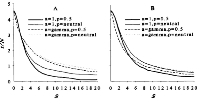
sented in Figure 3 in terms of the time to reach 90%

of 2, t o . @ ) , at the selection limit, as compared to the

same time for R , to,9(R).

When a is constant, Z approaches its limit more

rapidly than R for both

p

initially 0.5 and neutrally

distributed, reflecting the fact that the denominator

of (1 2 ) does not increase as fast as R. Variation of the

initial allele frequencies prolongs both to.9(Z) and

t O . g ( R ) . This is expected since the speed of increase of the mean and variance (related to the second moment) of selection response decreases as the initial allele frequencies deviate from 0.5.

When a varies among loci, is affected rela-

tively little, but t o . g ( Z ) increases significantly. When allelic effects are unequal among loci, a large propor- tion of the initial selection response is due to the alleles with relatively large effects. T h e change of the mean of the initial response is thus proportional to

1 0 1 2 1 4 1 6 1 8 2 0 S

FIGURE 3.-The time required to reach

90% of Z, hq(Z). (A) and R , to @), (B). T h e ;Illelic effect, a , is either 1 or gamma distrib- uted with = 1 , and the initial allelic fre- quency, p , is either 0.5 or neutrally distrib- uted with T = 20. Most calculations were done by using N = 20. For some large S

values N = 40 or 80 were used to improve precision.

the magnitudes of these allelic effects, but the change of the second moment is proportional to square of

these effects, so the denominator of ( 1 2 ) increases

faster than R. When initial allele frequencies also vary

among loci, to.g(Z) increases further.

These results are for unlinked genes. With linkage,

the transient behavior of 2 is very different.

Linkage effects

Linkage of genes influencing the character also

causes +i to underestimate the actual number of genes.

Its effect is two-fold. It reduces the divergent selection

response and also at the same time inflates 052. Linkage

inflates alf due to the linkage disequilibrium in the Fz

gametes,

where rlj is the recombination rate between loci i and

j . T h e reduction in response due to linkage is not very

significant for large numbers of chromosomes if genes

are randomly located in the genome (ROBERTSON

1970), but the inflation of a: can be substantial.

The linkage disequilibrium among genes in the high

and low lines brought about by selection also changes

a: by the amount

if alf is estimated as :,a

-

1/2(u;

+

a;), where D,j,, and

DtjI are the linkage disequilibria between loci i and j

in the high and low lines respectively. Our analysis indicates that this part of the effect is always trivial for populations initially in linkage equilibrium. In the

following analysis we exclude from a: the component

due to the linkage disequilibrium in the high and low lines.

Following the same argument leading to

(7)

and

be expressed as

which reduces to (1

2)

when genes are unlinked. Note

that the expectation is taken over the whole genome.

Considering the fact that genes located on different chromosomes are randomly associated, the expecta- tion can also be taken in two parts, within and between chromosomes, with appropriate weights. Suppose that

there are M haploid chromosomes in the genome with

the kth chromosome having the map length c k and

xgl

ck = C. Assuming the genes to be randomly

located in the genome, we expect that there are m ( m

-

1)

CEl

c : / C 2 within-chromosome pairs and m ( m

-

1)( 1

-

zEl

c:/C2) between-chromosome pairs among

m(m

-

1 ) pair joint-product terms [deduced from multinomial distribution]. Then the weight for the

within chromosome component is

Cf’I

c : / C 2 and for

the between-chromosome component is ( 1

-

2;1”=l

Equation 13 is a very complex function. Most of the

complexity is brought about by the unknown expected

allele frequencies with linkage. Before we analyze the behavior of this equation, let us first develop a limit- ing, but useful, argument about the selection limit.

Limiting argument: At the selection limit with

large S , Z can be approximated as

c:/c

2 ) .

by letting p l h r

-

pait + 1, where f is the average

recombination frequency between all pairs of loci. By our assumption of random allocation of genes in the genome, (1

-

2 ; )

= (2C

-

M

+

e - 2 ‘ k ) / ( 2 C 2 ) for

HALDANE’S (1 919) mapping function rii = 0.5( 1

-

) where dtj is the map distance between loci i and

j (FRANKLIN 1970). The above equation thus suggests

that, if m

>>

M ~ ( U ~ ) / [ ~ ( U ) ] ~ = M(l

+

p)/p,

i (= Z m ) has an upper bound

For example, if each chromosome has the same map length c (C = M c ) , this bound is 2c2M/(2c

-

1

+

e“‘).

For c = 0.5, 1 and 1.5 Morgan, it is 1.36M, 1.76M

and 2.19M respectively. Variation of chromosome map lengths will reduce this bound.

This expected upper bound is substantially less than the number of chromosome segments segregating in- dependently in one generation, i.e., the “recombina-

tion index” of DARLINGTON (1937), which equals the

haploid number of chromosomes plus the mean num- ber of recombination events per gamete. For instance,

Drosophila melanogaster has three regular chromo-

somes (with map length 0.66, 1.08 and 1.06 Morgan,

respectively) and a dot chromosome. Taking into ac- count that males have no recombination, our bound

is about 3.68, but the “recombination index” for

D.

melanogaster is 9. For maize, the bound is about 18

and the “recombination index” is 36 (LEWIN 1980).

However, Equation 14 is deduced by assuming that

genes are randomly located in the genome. Nonran-

dom distribution of genes will generally further lower

this bound. In the case of the equal spacing of genes

along the chromosomes, the expected upper bound is

the same as (1 4).

Theoretically, rit can exceed (14) by using the ge-

netic variance in FS, F4, or later generation popula-

t.ions to estimate a:, since the genetic variance in the

F2 population due to the linkage disequilibrium be-

tween loci i and

j

is reduced in each generation by a

proportion rij. Averaged over loci, the linkage dise-

quilibrium in F, ( t 2 _{2) generation is proportional to}

8[(1

-

r)f-2(1

-

2r)]

= - 4 2 1

-

4

c ( t

-

1)

-

1 1 - 1 ( t

;

1 ) 1 -2;-2Jc

c22t-yt

-

1) , = 1

for a chromosome with map length c, if genes are

assumed to be randomly located (see FRANKLIN 1970).

This rate of reduction is not as large as that given by the average recombination frequency between genes within chromosomes; but the linkage disequilibrium can still decrease substantially. There are, however, two disadvantages in using FS or later generation

variances to estimate a:, beyond the extra cost of

continuing experiments for more generations. First,

if the random mating population is not large, the

genetic variance is also expected to decrease due to drift. This part of the decrease needs to be corrected

in estimating a:. Second, as the genetic variance de-

creases, the sampling variance of estimates increases.

Returning to the effect of linkage on 2, w e need to

assess the expected value of Equation 13 under a

variety of assumptions. This was done by simulation.

SIMULATION

Methods

T h e simulations consisted of three parts: the for- mation of a base population with the desired param-

eters; the selection of replicate samples from this

population for high and low phenotypic values, which

Wright’s Estimator of Gene Numbers 24 1

means and variances for the parental, F1, and F2

populations, which we refer to as the estimation proc- ess.

T h e base populations were formed by assuming that

m loci were segregating for two alleles. Allelic effects

were either constant or drawn from a gamma distri-

bution with

0

= 1. Allele frequencies either started at

0.5 or were drawn from EWENS’ (1972) neutral allele

frequency distribution with 2T = 80. Loci were either

unlinked, or assigned map positions at random on chromosomes of length 100 cM. For pairs of loci on

the same chromosome, r was calculated using HAL-

DANE’S mapping function. For each replicate selection run, map positions, allelic effects and allele frequen- cies were chosen for each locus. T h e expected additive genetic variance was calculated, and the environmen-

tal variance, a:, was then chosen to yield either the

desired value of

S

= N ~ [ 2 ] ” ~ / a or a heritability, h 2 ,

of 0.25.

T o model the selection process, an initial sample of genotypes was drawn from this conceptual base pop- ulation, assuming gametic-phase equilibrium. Pheno- types were assigned by adding a random normal de-

viate with variance af to the sum of the allelic effects

for each genotype. Truncation selection for high and

low phenotypes was then carried out on this initial

sample. Gametes were drawn and combined at ran-

dom (with selfing permitted) from selected parents to yield offspring genotypes. T o model the estimation process, gametes were drawn at random from the

entire selection population to form n parental geno-

types, and then from these parents to form n F1 and

F2 individuals. T h e means and variances of the appro-

priate populations were then calculated.

f i was calculated in two ways. In the first case, the

genotypic values in the parental, F1 and F2 populations

were used to calculate

fi.

This estimate, called k g ,

includes the effects of linkage and gametic disequili- brium on the estimates, but ignores the sampling of

phenotypes. T h e second estimate, called m p , was cal-

culated from the sampled phenotypes, as in an actual experiment of this type,

(Ph

-

PJ

-

(ah‘

+

d ) / n

m,

=

Sa:

which is equivalent to equation (1) with a correction

for the numerator. T h e parameters a:, a;, and a:

were estimated using weighted least squares (COCK-

ERHAM 1986).

Results

Comparison of analytical and simulated re- sults: TO check the accuracy of our simulations and

the analytic results, we compared Z, calculated from

(1 I), with observed

.i?

and mg/m from simulations of

unlinked loci, where

kg

is the mean of Gg. These

comparisons are shown in Table

2.

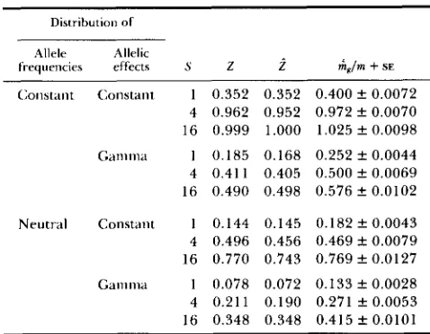
We consider selec-

TABLE 2

Comparison of analytical predictions (1 1) and simulations results for 10 unlinked loci

Distribution o f

Allele Allelic

frequencies effects S 2 i hgjm

+

SE

C;onstant Constant 1 0.352 0.352 0.400 f 0.0072 4 0.962 0.952 0.972 f 0.0070 16 0.999 1.000 1.025 f 0.0098

Ganlma 1 0.185 0.168 0.252 f O . 0 0 4 4

4 0.411 0.405 0.500 f 0.0069 16 0.490 0.498 0 . 5 7 6 f 0.0102

Neutral Constant 1 0.144 0.145 0.182 f 0.0043 4 0.496 0.456 0.469 f 0.0079 16 0.770 0.743 0.769 f 0.0127

Gamma 1 0.078 0.072 0.133 f 0.0028 4 0.211 0.190 0.271 f 0.0053 16 0.348 0.348 0.415 k 0.0101

For a given S value, the total population size and the proportion selected were chosen to yield a reasonable heritability. For S = 1 , 4, and 16, the total population size was 10, 20, and 60; the proportion selected was 0.2,0.5 and 0.5; and simulation replications were 1000, 500 and 200, respectively.

tion to fi5ation for populations initially segregating at

10 loci. 2 was obtained by substituting observed av-

erage fixation probabilities and allelic effects into

equation

(7).

T h e observed agrees well with the

expected Z. As exeected from comparison of equa-

tions (4) and (7), 2 5 mg/m in most cases, and the

estimates of mg/m exceed

.i?

by something less than

l/m. These results even hold for unequal allelic effects and initial frequencies.

Linkage effects: T h e effects of linkage were inves-

tigated by simulations utilizing 10 loci, which were

assumed to be either unlinked, or randomly distrib-

uted on one, three or ten chromosomes. Figure 4

shows the ratio mg/m at fixation as a function of S . As

expected, linkage substantially reduces mg/m. In the

extreme case where all ten loci are distributed in one chromosome, linkage essentially dominates the esti- mation; population size, selection intensity, allelic ef- fects, and allele frequencies all become unimportant.

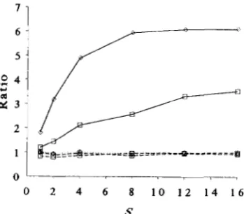
Figure 5 shows the ratios of observed components

of 2, calculated as in Equation 13, with all ten loci on

a single chromosome to that when all loci are un-

linked. T h e ratio of components for the selection

response ([( p z h

-

pS)(

p j h

-

fijl)a,a,

I),

and for the

added F2 genic variance ([( p i h

-

p i l ) a i ] 2 ) are approxi-

mately one, while the denominator of (13), the real- ized added F2 genetic variance (including linkage dis- equilibrium), is substantially increased with linkage.

This agrees with ROBERTSON’S (1970) conclusion that

linkage tends to have small effects on selection re-

sponse. T h e reduction in

hg

from linkage is essentially

all due to linkage disequilibrium in the F1 gametes.

D. Houle

l ' O

1

7

bo

"'

0 . 4 -

0 . 2

0 . 0 ' " ' ' ' ~ ' ~

0 2 4 6 8 10 1 2 1 4 1 6 S

FIGURE 4.-The effect of linkage on &/m at fixation when m = 10. Thick solid lines denote unlinked loci, thin solid lines loci randomly located on ten chromosomes, dashes three chromosomes, dotted lines one chromosome. Diamonds denote cases where allelic effects are assumed to be equal and initial allele frequency is 0.5. Squares denote cases where allelic effects were drawn from the gamma distribution with p = 1, and allele frequencies were drawn from the EWENS' distribution (T = 40). To achieve a given S value while preserving a reasonable heritability, the total population size during selection and the proportion selected were varied. T h e proportion selected was 0.2 for S = 1 and 0.5 otherwise. For S

values 1, 2, 4, 8, 12, and 16, the total population size was chosen to be 10, 10, 20, 30 and 40, respectively. Selection replicate numbers were 300, 250, 200, 100, 100 and 100, respectively.

know the magnitude of S in his experiments because

the actual number of loci, their allele frequencies, and allelic effects are unknown. However, the number of chromosomes will usually be known, and heritability may be estimated. Consequently a clearer idea of the utility of this method is gained by examining the effect

of changing the actual number of loci, m, on rii when

chromosome number and heritability are fixed. Fig-

ure 6 shows m g as a function of m for three linkage

regimes. With linkage, as m increases, m g underesti-

mates m by a greater and greater amount, and be-

comes nearly constant. Consequently, when m

>

M,

m g is quite insensitive to the actual number of loci.

Note that does not become very close to the upper

bound implied by Equation 14, even when there are

20 loci on only three chromosomes. For constant map

length of 1 Morgan assumed here, the upper bound

is 5.3 for M = 3, and 17.6 for M = 10. These results,

borne out by additional simulations not shown, indi- cate that m g = M when m

>

M .

With linkage, the time required to obtain 90% of

the limiting value of Z, to.&), is shorter compared

with that with random recombination, especially when S is small or m is large. Also, t o . g ( Z ) is much less than

with linkage (Table 3). This is partly because

the expected 2 is smaller with linkage and partly

because linkage disequilibrium in the F:! after crosses of high and low lines builds up gradually as selection proceeds and linkage has little effect on selection response.

7 1

2

4 -

2

3 -

Y

2 -

1 -

0 2 4 6 8 1 0 1 2 1 4 1 6

, 77

S

FIGURE 5.-Ratio of components of 2 at fixation when ten loci are linked on a single chromosome to that when ten loci are unlinked. Dotted lines denote the numerator of Equation 13, dashed lines [ ( p , h - p,,)a,I2, the genic F:! variance, and solid lines the

denominator of Equation 13. Diamonds indicate equal allele fre- quencies and effects, and squares variable allele frequencies and effects, as described in the legend of Figure 4. Populations sizes are as in Figure 4. Selection replicate numbers were 1,000, 1,000, 500.

300, 300 and 200 for the six S values graphed.

Sampling variance of tii:There are three sources of sampling which contribute to the sampling error of

estimates of rii in our simulations. They are (i) the

sampling of the initial population (initial allele fre-

quencies, effects, and map positions); (ii) the variation

in chance of fixation of alleles; and (iii) the sampling

of phenotypic observations. Table 3 shows the ob-

served standard deviations of estimates of rii from

simulations. An estimate, G G ~ , of standard deviation

of riz given by LANDE (1981), which approximates the

sampling standard deviation in the process of estima- tion, is also listed in the Table. Generally the standard

deviation of

rii,,

ukp, is large and can be very large

when m

<

M , so m p , the mean of m p , may be very far

from

kg.

This large variance is not primarily due to

the sampling of parameters or to the selection process.

With samples of the size we have used, the sampling variance due to the sampling of genetic parameters

and selection process, ai-, is usually small and can be

ignored. In almost all cases it accounts for less than

1% of the variance. T h e enormous variance of mf is

largely due to a small number of cases where a: is

very near 0, leading to estimates of

kP

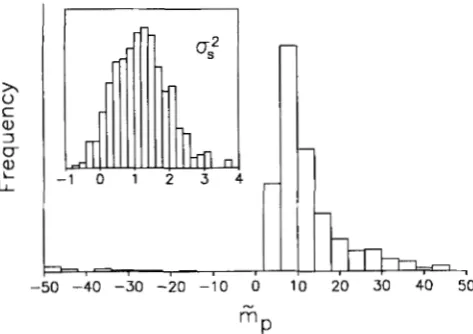
with very large

absolute values. Typical distributions of observed a:

and riip are plotted in Figure 7. The distribution of us

is not significantly different from normal, but overlaps

zero. This suggests that simply discarding those few

estimates of a, with negative or very small values might

substantially improve precision. Table 3 also shows

summary statistics when all values of h i p which are

negative or more than 100 are discarded. This does indeed lower the variance, but also slightly biases the

mean upward. As CARSON and LANDE (1 98 1) pointed

out, the problem of a, overlapping 0 leads LANDE'S

Wright's Estimator (

1 5 -

ca

"I8 1 0 -

5 -

0 ' " " " " "

0 2 4 6 8 1 0 1 2 1 4 1 6 1 8 2 0 m

FIGURE 6.-hg as a function of m. Lines were selected until

fixation or 200 generations had passed. Thick solid lines are for unlinked loci, thin solid lines for ten chromosomes, and dashed lines for three chromosomes. Diamonds denote equal allelic effects and frequencies, and squares variable allelic effects and frequencies. Values are means of 300 replicates.

observed variance. This is true even after the data is censored and when the variance due to sampling of genetic parameters and selection is removed.

Since the variance due to the selection process is relatively small, we investigated the effect of obtaining replicates from the same selected populations, then

using averaged estimates of the numerator and de-

nominator to obtain m p . We simultaneously investi-

gated the effects of estimation replicate sample size n

and replicate number y on ckp for a fixed total sample

size ny. T o d o this, we used a slightly different simu-

lation scheme, which does not include the selection

process. In these simulations, loci were assumed to have previously been fixed for appropriate alternate

alleles. T h e environmental variance was chosen so

that a population which segregated for the allelic

effects represented, assuming either equal initial fre- quencies or neutral initial frequencies, would have a

heritability of 0.25. Estimates of a,' and (ph

-

pr)2

were calculated by weighted least squares within each

replicate, then averaged over y replicates. Figure 8

summarizes the results with m = 20. T h e total sample

size shown in the abscissa is n times y. T h e value of y

can then be seen by dividing ny by n, depicted in the

figure. For example, for the curve of n = 32, y ranges

from 1 to

7.

T h e standard deviations in the figure

were calculated from at least 200 observations.

For unlinked loci, in part A of Figure 8, ckP de-

creases almost linearly with ln(ny). For a given number

of individuals measured, ukp decreases somewhat if

those individuals are analyzed in several replicates. However, there is still substantial variance, even at the largest total sample size, 2048. Unless sample size

is approximately 500 or more, the empirical confi-

dence intervals of

mp

do not, on the average, exclude

0. T h e situation is somewhat different for the case

where all 20 loci are assumed to fall on three chro-

If Gene Numbers 243

mosomes, as in part B of Figure 8. Here replication

during estimation has less effect. Increasing sample

size beyond 5 12 has little effect. With three chromo-

somes, the genome behaves like three loci, each with

relatively large effects. This reduces both

hip

and ukp.

DISCUSSION

Our results suggest that WRIGHT'S method is of

little value in estimating the number of loci influenc- ing a quantitative character. Linkage effectively pre- vents the expectation of such estimates from exceed- ing the number of chromosomes, and sampling vari- ance may easily prevent one from concluding that the number of loci is even that large.

Ironically, our results also show that divergent se- lection is useful to validate the assumption of

WRIGHT'S method for estimating the number of loci

that high and low valued alleles are fixed in the

appropriate populations. However, for the reasons

given above, the many estimates of the number of

genes based on WRIGHT'S method using one way or

divergent selection must still be considered suspect. The problem of linkage may be partially compen-

sated for if we use the variances from F3 or later

generations for estimating a,', instead of the F2 vari-

ance. T h e gametic disequilibrium in the F2 will be

reduced by recombination, which allows a,' to ap-

proach the genic variance in the population, and the

value of i will increase correspondingly. T h e value

of this approach is counteracted by drift in the hybrid populations. It has been suggested that the additive genetic variance in the base population can be used as

an estimate of a,', which may be free from the influ-

ence of gametic disequilibrium (COMSTOCK 1969;

PARK 1977a; FALCONER 198 1). This requires, how-

ever, that the allele frequencies in the base population

be known. T h e only case when this could be true is following a cross between completely inbred lines, which would itself introduce disequilibria in the pop- ulation.

Sampling variance of the estimate is the second major problem with WRIGHT'S method. Part of the

problem is that the denominator of Equation 1 can

easily be negative, or very small. This is particularly true with short term selection lines which have not

diverged enough. This problem will be substantially

less if the parental means are many phenotypic stand-

ard deviations apart, as is true for the examples in

LANDE (1981). When negative estimates occur, it is

usually interpreted as a violation of some assumptions, rather than a possible consequence of sampling vari- ance. When such estimates are simply discarded, this biases the remaining sample. Both large sample size and replications of the estimation process are useful in preventing this. With replication, we have shown

TABLE 3

Effect of phenotypic sampling during estimation

Censored 0 < + L ~ < 100

Genera- tions to

90% o f

frequency” M m mg mP d, a - “g aip ZP u*p P(OK)d 2 R

Allelic effects,

Constant m 3 3.036 17.575 0.000 0.397 173.233 1.872 5.390 8.464 0.943 3 6 20 18.607 76.932 1.215 3.044 573.554 4.704 20.806 13.700 0.897 13 17

10 3 2.805 8.151 0.415 0.569 46.372 1.568 4.745 8.643 0.970 3 6

20 9.527 10.685 1.256 1.824 41.092 1.404 11.554 7.712 0.993 10 17

3 3 2.322 1.907 0.507 0.572 66.750 1.084 2.977 2.904 0.957 2 6 20 4.432 4.688 0.460 0.732 1.576 0.411 4.688 1.380 1.000 6 17

Variable m 3 1.721 1.985 0.608 0.645 4.405 0.684 2.093 1.620 0.973 5 5 20 5.808 5.349 1.601 1.784 107.341 0.909 6.976 5.605 0.973 13 12

10 3 1.646 1.889 0.532 0.575 33.966 0.608 1.989 1.751 0.987 5 5

20 4.583 4.627 1.233 1.379 57.503 0.692 6.172 8.053 0.983 1 1 12 3 3 1.480 2.490 0.481 0.513 10.270 0.538 1.820 1.667 0.970 4 6

20 3.018 3.224 0.625 0.753 2.824 0.363 3.357 1.663 0.997 9 12

Three hundred replicates of the selection process for each parameter set were generated. The best 8 out of 40 individuals were chosen during the selection process, which continued until fixation or 200 generations had passed. For estimation samples of 100 individuals in the parental, F, and F.L populations were used. Heritability was assumed to be 0.25 in the base population.

a Constant: p = 0.5, a = 1; Variable: p from EWENS’ distribution, and a gamma distributed.

* Standard deviation of G assuming infinite sample size during the estimation process. ‘ Expected standard deviation of Gp from LANDE’S approximate formula.

Proportion of replicates where 0 < G, < 100.

I

- 1 0 1 2 3

1

7

4

r

-50 -40 -30 -20 -10 0

“P

-

k

10 20 30 40 50

FIGURE 7,”Typical distributions of observed cry and Gp from simulations. Allelic effects and frequencies were assumed to be equal initially. The total population size during selection is 40. The proportion selected is 0.2. m = 10. n = 100. Simulations were run until fixation or 200 generations passed. Of the 500 replicates obtained, 12 yielded values of 6, C -50 and 32 estimates > 50.

Equation 1 over replicates decreases the variance of

&. However, one of the appealing features of WRIGHT’S method is that it can be estimated from data commonly collected. If experimentalists are will- ing to spend considerable efforts attempting to esti-

mate the number of genes, we feel that it would be

best to investigate alternative methods using genetic

markers (see below), rather than doing large repli-

cated crosses of the sort we have investigated.

LANDE (1981) has given an approximate sampling

variance for estimates of & which takes into account

only the variation stemming from the process of esti-

mation, assuming that a: is greater than 0. With

divergent selection, the variation in selection response also contributes to the sampling variance of the esti- mate. T h e small magnitude of the selection replicate standard error presented in Table 3 suggests that this additional source of error is not large for reasonable parameter combinations. Even allowing for this, the

values in Table 3 make it clear that LANDE’S sampling

variance substantially underestimates the actual vari-

ance. T h e large discrepancies in Table 3 are due to

estimates of very large absolute value when a: is near

0. However, approximately 90% of our estimates do

lie within two of LANDE’S standard errors of the ex-

pected value of

6

(results not shown), which is in

agreement with CARSON and LANDE’S (1984) analysis

based on bootstrapping resampling. So Ghp does have

some utility in assessing the reliability of m p .

One positive result from our analysis is that selec- tion can rapidly generate populations whose expected

6 are close to those at fixation. T h e expected value

of

6

initially approaches its limit more rapidly than

selection response does. T h e half-life of selection re-

sponse for typical selection experiments is about 0 . 2 N

to 0.4N generations (FALCONER 198 1). For & the half-

life is usually less than 0 . 2 N generations for S

>

4.

The 90% life for 6 is usually less than 1.5N genera-

tions, especially in the presence of linkage (Table 3).

Wright’s Estimator of Gene Numbers 245

0 0.0

-

FIGURE 8.”Standard deviation of

k p , censored to exclude values of

k, c -100 or >loo, for rn = 20, as a function o f replicate size, n, and esti- mation replicate number, y. Allele fre- quencies m d effects are assumed equal. Part A is for unlinkled loci, and part B is for three chromosomes. Lines are labeled with values of n.

See text for further explanation.

2 0 1 0 0 1 0 0 0 2 0

BY

modest effective population sizes, less than 10-20

generations of selection are enough to achieve most

of the limiting estimate of

7ii.

Selection for longer than

this does not provide much gain based on the original

genetic variation. Longer selection will tend to include

the variation due to new mutations (HILL 1982; EN-

FIELD and BRASKERUD 1989).

We have ignored two common features of genetic systems in this paper. T h e first of these is dominance, and the second is natural selection. Both would tend to prolong the time to approach limiting estimates of

7ii as alleles with deleterious effects tend to be reces-

sive. Dominance may either increase or decrease the

expectation of rii (MATHER and JINKS 1982), while

countervailing natural selection will usually decrease

it by preventing fixation of deleterious alleles. How-

ever, both of these effects would tend to be overshad- owed by linkage if the number of loci is large.

In addition to WRIGHT’S method, there are also

many other statistical methods of gene number esti-

mation, in particular those of PANSE (1 940),JINKS and

TOWEY (1 976) and COMSTOCK and ENFIELD (1981).

Some statistical methods are just variations of

WRIGHT’S method, sharing some of its properties and

problems (e.g., STUDENT 1934; COMSTOCK 1969; PARK

1977a,b; FALCONER 198 1). Compared with WRIGHT’S

method, PANSE’S method, which uses the variance of

the Fa generation, does not have much advantage,

and is more sensitive to changes in the parameters,

and more laborious to estimate (MATHER and JINKS

1982). COMSTOCK and ENFIELD (1981) proposed a

method to estimate gene number with multiplicative gene effects, which also uses divergent selection and subsequent crosses. They did not analyze the effect of linkage on the estimate. This effect must be large

since the genetic variance in the base population,

which results from a cross between two inbred lines, is used, and the biases caused by deviations from the

assumptions are unknown. MAYO and HOPKINS (1 985)

showed that this method has the problem that it is

very sensitive to small changes in the parameters.

JINKS and TOWEY’S method involves the determina-

tion of the proportion of individuals in the F, gener-

ation of a cross between two inbred lines that are

1 0 0 1 0 0 0

nY

heterozygous at one locus, at least, by an assay of their

Ft+2 grandprogeny families. They assume that prog- eny from the F2 generation on are obtained by selfing.

As t increases, the estimate increases, because of re-

combination.JINKS and TOWEY’S method tends to give

larger estimates than WRIGHT’S method in their ex-

periments, but is still a kind of minimum as it is under

the influence of linkage (HILL and AVERY 1978). T h e

estimate has the problems that it is much susceptible

to selection for heterozygotes or against deleterious

recessives at linked genes (HILL and AVERY 1978). It

is also very sensitive to unequal allelic effects and

becomes very inaccurate for large gene number

(MAYO 1987).

While animal and plant breeders need to be most concerned with loci which currently segregate in pop-

ulations, the goal of estimating gene number in an

evolutionary context is yet one step more complex. In

the long term, it is the number of loci capable of

expressing the type of variation studied which is of

interest, rather than just the number which currently

do. Even with a good estimate of the number of loci

segregating in a population, it is necessary to make

assumptions about the mechanisms maintaining that variation, including such factors as effective popula-

tion size, in order to estimate the number of loci

capable of influencing the character.

Estimation of gene number is a long standing prob- lem. Despite its obvious importance in animal and

plant breeding and in understanding evolutionary

processes, we are still painfully short of a reliable

method to do it. This is discouraging for all of us who depend on such estimates to design and perform ex- periments or build models. There may be no practical

alternative to the enumeration of loci using expensive,

labor-intensive techniques that utilize genetic markers

(SAX 1923; THODAY 196 1 ; TANKSLEY, MEDINA-FILHO

and RICK 1982; EDWARDS, STUBER and WENDEL

1987; PATERSON et al. 1988; LANDER and BOTSTEIN

1989). In particular, the quantity of molecular mark- ers which we can now imagine locating makes efforts of this kind conceivable. However, since the technique

can only locate genes segregating for alleles with

of distributions of allelic effects before we can estimate the number of genes.

We thank TRUDY MACKAY and two reviewers for their com- ments, and J. POOLE for assistance in making figures. This investi- gation was supported in part by research grant GM 1 1546 from the National Institute of General Medical Sciences.

LITERATURE CITED

CARSON, H. L., and R. LANDE, 1984 Inheritance of a secondary sexual character in Drosophila silvestris. Proc. Natl. Acad. Sci. USA 81: 6904-6907.

CASTLE, W . E., 1921 An improved method of estimating the number of genetic factors concerned in cases of blending inheritance. Science 54: 223.

COCKERHAM, C . C., 1986 Modifications in estimating the number of genes for a quantitative character. Genetics 1 1 4 659-664. COMSTOCK, R. E., 1969 Number of genes affecting growth in

mice, pp. 137-148 in Genetic Lectures. Oregon State University, Corvallis.

COMSTOCK, R. E., and F. D. ENFIELD, 1981 Gene number esti- nlation when nlultiplicative genetic effects are assumed- growth in flour beetles and mice. Theor. Appl. Genet. 59: 373-379.

DARLINGTON, C . D., 1937 T h e biology of crossing-over. Nature 140: 759-761.

EDWARDS, M . D., C. W. STUBER and J. F. WENDEL, 1987 Molecular-marker-facilitated investigations of quanti- tative trait loci in maize. 1. Numbers, genomic distribution and types of gene action. Genetics 116: 113-125.

ENFIELD, F. D., and 0. BRASKERUD, 1989 Mutational variance for pupa weight in Tribolium castaneum. Theor. Appl. Genet. 77: 41 6-420.

EWENS, W. J., 1972 T h e sampling theory of selectively neutral

FALCONER, D. S . , 1981 Introduction to Quantitative Genetics, 2nd

FRANKLIN, I . R., 1970 Average recombination frequencies. Ge-

HALDANE, J. B. S., 1919 T h e combination of linkage values, and the calculation of distance between loci of linked factors. J.

Genet. 8: 299-309.

HILI., W. G., 1982 Predictions of response to artificial selection

HILL, W. G., and P. J. AVERY, 1978 O n estimating the number of genes by genotype assay. Heredity 40: 397-403.

HILL, W. G., and J. RASBASH, 1986 Models of long term artificial selection in finite population. Genet. Res. 48: 41-50.

JINKS, J. L., and P. M. TOWEY, 1976 Estimating the number of genes in a polygenic system by genotype assay. Heredity 37: 69-8 1 .

KIMURA, M., 1957 Some problems of stochastic processes in ge-

KIMURA, M., 1979 Model of effectively neutral mutations in which alleles. Theor. Popul. Biol. 3: 87-1 12.

Ed. Longman, London.

netics 66: 709-7 l l .

from new mutations. Genet. Res. 40: 255-278.

netics. Ann. Math. Stat. 28: 882-901.

selective constraint is incorporated. Proc. Natl. Acad. Sci. USA 76: 3440-3444.

LANDE, R., 1981 T h e mininlum number of genes contributing to quantitative variation between and within populations. Ge- netics 99: 541-553.

LANDER, E. S . , and D. BOTSTEIN, 1989 Mapping Mendelian fac- tors underlying quantitative traits using RFLP linkage maps. Genetics 121: 185-199.

LEWIN, B., 1980 Gene Expression. Vol. 2 , Eucaryotic Chromosomes.

MATHER, K., and J. L. JINKS, 1982 Biometrical Genetics, 3rd Ed.

MAYO, 0.. 1987 The Theory of Plant Breeding, 2nd Ed. Clarendon,

MAYO, 0.. and A. M. HOPKINS, 1985 Problems in estimating the minimum number of genes contributing to quantitative varia- tion. Biom. J. 2: 181-187.

PANSE, V. G . , 1940 Application of genetics to plant breeding. 11.

T h e inheritance of quantitative characters and plant breeding.

J. Genet. 40: 283-302.

PARK, Y . C., 1977a Theory for the number of genes affecting quantitative characters. 1. Estimation of and variance of the estimates of gene number for quantitative traits controlled by additive genes having equal effect. Theor. Appl. Genet. 50:

153-161.

PARK, Y . C., 1977b Theory for the number of genes affecting quantitative characters. 11. Biases from drift, dominance, ine- quality of gene effects, linkage disequilibrium and epistasis. Theor. Appl. Genet. 5 0 163-172.

PATERSON, A. H., E. S. LANDER, J. D. HEWITT, S. PETERSON, S. E. LINCOLN and S. D. TANKSLEY, 1988 Resolution of quantita- tive traits into Mendelian factors by using a complete RFLP linkage map. Nature 335: 721-726.

ROBERTSON, A., 1970 A theory of limits in artificial selection with many selected loci, pp. 246-288 in Mathematical Topics in Population Genetics, Vol. 1 , edited by K. KOJIMA. Springer- Verlag, Berlin,

SAX, K., 1923 T h e association of size differences with seed-coat pattern and pigmentation in Phaseolus vulgaris. Genetics 8: 552-560.

SHULL, G. H., 1921 Estimating the number of genetic factors concerned in blending inheritance. Am. Nat. 55: 556-564. STUDENT, 1934 A calculation of the minimum number of genes

in Winter's selection experiment. Ann. Eugenics 6: 77-82. TANKSLEY, S. D . , H. M E D I N A - F I L H O ~ ~ ~ C. M. RICK, 1982 Use of

naturally-occurring enzyme variation to detect and map genes controlling quantitative traits in an interspecific backcross of tomato. Heredity 49: 11-25.

THODAY, J. M., 1961 Location of polygenes. Nature 191: 368- 370.

WRIGHT, S., 1968 Evolution and the Genetics of Populations. V o l . 1 . Genetics and Biometrical Foundations. University of Chicago Press, Chicago.

John Wiley 8c Sons, N e w York.

Chapman 8c Hall, London.

Oxford.

Communicating editor: A. G. CLARK

APPENDIX

C. J. JIANG

Let the allelic effect, a, and initial frequency,

p ,

be of fixation for the loci can be summarized as follows:

constant over loci. At the selection limit, the outcome

Wright's Estimator of Gene Numbers 247

where uh and ul are the probabilities of an allele with

effect a being fixed in the high and low lines respec- tively. Thus uh

-

U I = (x

-

?)a, a: = (x

+

y)a2/8 and

m = - (x

-

r)'

X + Y

By the assumption that the fixation status of one locus

is independent of that at other loci, x and y are

trinomially distributed with the probability

Pr(x, y

I

m ) = m! PXQY( 1

-

P

-

Q)"-"'.

x ! y ! ( m - x -y)!

Since

= m ( P

+

Q )

-

48-

X + y '

we need only evaluate the last term.

8- XY

X + Y m

= x -

XY m !

x

+

y x ! y ! ( m

-

x

-

y)!

P"QY(1

-

p

-

Q)"Y

= P Q

i

-

1 m !

X

+

y (x

-

l ) ! ( y

-

l ) ! ( m

-

x

-

y)! pX-1Qu-l(l

-

p

-

Q)m-x-y

Letting w = (x

-

1 )

+

(y

-

1 ) and P I = P

+

Q and

translating the trinomial distribution of x and y to

binomial distribution of w give

m-2

1 m

= P Q

x

-

e(

1

-

Pl)""'

e+'(

1

-

Pl)m-w-2

w=o w

+

2 w!(m

-

w

-

2)!

(w

+

l)m! (w

+

2)!(m

-

w

-

2)!

(w

+

2

-

l)m! py+2(1

-

p l ) m - w - 2 (w

+

2)!(m

-

w

-

2)!

-

(0

-

1)- PY(1 -PI)"

-('

-

l ) l ! ( m

-

I ) ! PI( 1

-

Pl)m-l

m! O!m!

m!

=-" mpQ PQ ( 1 - ( 1 -P-Q)"). P + Q (P+Q)'

Thus

8(6)

= m(P

-

Q)' I 4 ~ 4

P + Q ( P +

Q )

'[ 1

-

( 1

-

P

-

Q)"].

T h e ratio of expectations is

8 ( x

-

y)2 8(x

+

Y)

& , =

Since

p (

1

-

p )

5 P 5 1 and 0 5 Q 5

p (

1

-

p ) ,

it is easy to show that