Study on the Relations between Subsurface Structure and Variability of Strong Ground Motions at Adjacent Sites

(1)

Study on the Relations between Subsurface Structure and

Variability of Strong Ground Motions at Adjacent Sites

Ryoichi Tokumitsu1_{, Yu Yamamoto}2_{, Yasuo Uchiyama}3

1 _{Senior Research Engineer, Technology Center, Taisei Corporation, Japan (tkmrui00@pub.taisei.co.jp)} 2 _{Senior Research Engineer, Technology Center, Taisei Corporation, Japan}

3 _{Chief Research Engineer, Technology Center, Taisei Corporation, Japan}

ABSTRACT

Effects of subsurface soil structure on the spatial variability of ground motions between adjacent sites are examined using observed records from the Chiba Array and pairs of the K-NET and the KiK-net seismic network, Japan, which are adjacent to each other. The statistical analysis of coherence of the ground motion showed that the spatial variability of ground motion depends on subsurface soil structure and the decrease in P and S-wave velocity of subsurface soil causes a reduction of spatial coherence. We also found that the longer the distance between observation sites, the deeper the soil properties effect on the spatial variability of ground motions.

INTRODUCTION

Spatial variability of strong ground motions at adjacent sites would cause significant effect on the dynamic response of large structures; e.g. the reduction in high frequency components of input motions and the increase of the rocking or torsional responses (Luco et al., 1986).

Characteristics of spatial variability of ground motion have been studied by observation records analysis at adjacent sites. Many researchers have pointed out that spatial variability becomes larger as frequency is higher. They also indicate that the longer the distance between the sites, the larger the spatial variability of ground motion becomes. Based on these analyses, some empirical equations of spatial variability have been proposed as a function of frequency and distance between sites as parameter (Harichandran et al., 1986; Hao et al., 1989; Nakamura et al., 1995; Abrahamson et al., 2006).

Another parameter that effects on spatial variability of ground motion would be subsurface soil structure, but the relation between the soil properties and spatial variability of ground motion has not been completely cleared. Somerville et al. (1991) and Schneider et al. (1992) point out that there are differences in spatial variability between alluvial and rock, while Chiu et al. (1995) concludes that subsurface soil condition does not make considerable effects on spatial variability.

(2)

GROUND MOTION RECORDS

In this study, we use seismic records of the Chiba Array system, University of Tokyo, and pairs of observation sites from the K-NET and the KiK-net seismograph network by the National Research Institute for Earth Science and Disaster Resilience, Japan (NIED).

In the Chiba Array system, seismographs had been installed on the ground surface showed in Figure 1 (Katayama et al., 1990). The minimum distance between seismographs is 5 meters and the maximum distance is about 300 meters. Seismic records observed in the Chiba Array system from 1982 to 1992 are offered by the Association for Earthquake Disaster Prevention, Japan.

The K-NET consists of about 1000 seismographs which are installed on the ground surface and distributed every 20km uniformly covering Japan. The KiK-net consists of pairs of seismographs installed in a borehole and on the ground surface, deployed at approximately 700 locations nationwide. More than 20 years have passed since both seismograph networks installed and many seismic records have been observed. Among K-NET and the KiK-net networks, there are some observation sites but very rarely that adjacent to each other whose distance is less than 100 [m]. We use the records observed at the pair of K-NET and the KiK-net showed in Table 2 from the beginning of operation to 2017 for this study. Table 2 also shows the distance between the pair of K-NET and the KiK-net observation sites. The location of these observation sites is shown in Figure 2.

Figure 1: Location of Seismographs in Chiba Array

Table 1: Pairs of Seismographs in Chiba Array

Distance between Seismographs Pairs of Observation Sites Distance Class

5m C0-C1, C0-C2, _{C0-C3, C0-C4} 1

7m C1-C2, C1-C4, C2-C3, C3-C4 2 15m C0-P1, C0-P2, _{C0-P3, C0-P4} 3 30m P1-P3, P2-P4 4

67m P6-P7 5

Table 2: Pairs of Observation Sites of K-NET and KiK-net for This Study

Distance between Seismographs

Pairs of

Observation Sites Distance Class K-NET KiK-net

4m HKD130 IBUH05 1 4m TYM012 TYMH07 4m YMN008 YMNH09 5m HKD084 KSRH02 6m HKD090 TKCH05

2 8m GIF001 GIFH13

15m MIE014 MIEH05 3 29m HKD142 SBSH03 4

60m HKD123 SRCH10 5 _{Figure 2: Location of K-NET and KiK-net} Observation Sites for This Study

(3)

Class 1 Class 2 Class 3

Class 4 Class 5

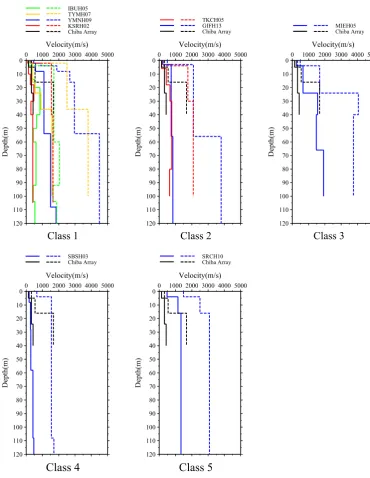
Figure 3. Subsurface P and S-wave Velocity Structures by Distance Classes

In this study, pairs of observation sites are classified in five according to the distance between observation sites. Distance classes of each pair of observation sites are listed in Table 1 and 2. Figure 3 shows the subsurface soil velocity structures of each site by distance classes (NIED; Katayama et al., 1990). Solid lines show S-wave velocity and dotted lines show P-wave velocity.

To avoid the effects of magnitude and hypocentral distance on the spatial variability, only records of JMA magnitude (MJ) 5.5 – 6.5 and hypocentral distance 50 – 200 [km] are used in this study. The

numbers of seismic events at each pair of observation sites that satisfy the range of magnitude and distance above are listed in Table 3.

IBUH05 TYMH07 YMNH09 KSRH02 Chiba Array

SBSH03

Chiba Array SRCH10 Chiba Array TKCH05 GIFH13

(4)

Table 3. Numbers of Seismic Events for This Study

Pair of

K-NET, KiK-net Num. of Events K-NET, KiK-netPair of Num. of Events Pairs of Chiba Array Observation Sites Num. of Events HKD130-IBUH05 15 GIF001-GIFH13 3 Class 1 7 TYM012-TYMH07 6 MIE014-MIEH05 8 Class 2 7 YMN008-YMNH09 8 HKD142-SBSH03 5 Class 3 7 HKD084-KSRH02 37 HKD123-SRCH10 10 Class 4 7

HKD090-TKCH05 41 Class 5 5

In this study, we analyse the spatial variability of ground motion for horizontal and vertical component of S-wave as well as vertical component of P-wave. For the analysis of S-wave, 10.24 seconds of waveforms from the beginning of S-wave are obtained. For the analysis of P-wave, we obtain 5.12 seconds of waveforms from the beginning of P-wave or the beginning of the data. Both ends of 0.5 seconds of each waveform are filtered by cosine taper.

CHARACTERISTICS OF SPATIAL VARIABILITY

In this study, spatial variability of ground motion is quantified by coherence. Coherence of ground motion between the observation site i and jCoh f is described by equation (1).

Coh f _N1 G f

G f G f (1)

Where f is frequency, G f is the cross spectrum between the observation site i and j of the seismic event m, G f and G f are power spectrum of the observation site i and j of the seismic event

m, and N is the total number of seismic events. Cross spectra and power spectra are smoothed with Parzen window at 1.0 [Hz]. Coh f of horizontal component of S-wave is derived from the average of

Coh f of radial and transverse components of ground motion. Coh f of horizontal component of S-wave are shown in Figure 4 and Coh f of vertical component of S-wave are shown in Figure5 and

Coh f of vertical component of P-wave are shown in Figure 6.

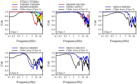
Coh f of vertical component of P-wave in Figure 6 are larger than Coh f of horizontal and vertical component of S-wave in Figure 4 and 5. There is no significant difference between Coh f of horizontal and vertical components of S-wave.

(5)

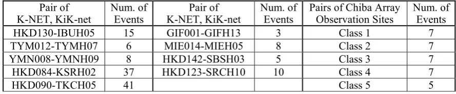
Figure 4. S-wave Coherence of Horizontal Component by Distance Classes (Frequency Domain)

Figure 5. S-wave Coherence of Vertical Component by Distance Classes (Frequency Domain)

HKD130-IBUH05 TYM012-TYMH07 YMN008-YMNH09 HKD084-KSRH02 Chiba Array (Class 1)

HKD090-TKCH05 GIF001-GIFH13

Chiba Array (Class 2) MIE014-MIEH05 Chiba Array (Class 3)

HKD142-SBSH03

Chiba Array (Class 4) HKD123-SRCH10 Chiba Array (Class 5)

HKD142-SBSH03

(6)

Figure 6. P-wave Coherence of Vertical Component by Distance Classes (Frequency Domain)

On the other hand, Coh f are significantly different even though in the same distance class. To take distance the class 1 as an example, Coh f of YMN008-YMNH09 is highest and Coh f of HKD084-KSRH02 or Chiba Array are lower than other pairs of observation sites in Figure 4-6. According to the subsurface velocity structures in Figure 3, P and S-wave velocities in YMNH09 are higher than those in KSRH02 or Chiba Array. Considering from these results, Coh f tends to maintain high degree as the P and S-wave velocity of subsurface soil is higher.

In high-velocity subsurface structure, seismic wave propagates with long wavelength and less wavenumber, so seismic waves would be hard to be scattered and Coh f could get higher relatively. That is to say, it could be inferred that the residuals of Coh f between pairs of observation sites in the same distance classes decrease by transferring frequency domain Coh f into waveform domain to the depth of subsurface soil that have strong effects on the spatial variability h .

To confirm these presumption, we defined h by transferring Coh f into wavenumber domain function Coh k and compared Coh k in the same distance class with each other. The method of defining h is described as follows.

1) Subsurface velocity structure at the depth of 0-h [m] of each observation site is set according to Figure 3. In this study, we defined h as 150 [m]. In case there is no information of velocity structure to the depth of h , the same value at the deepest point of velocity structure in Figure 3 is set up to the depth of h .

2) The average velocity at the depth of 0-h [m] AV is computed from the subsurface velocity structure described in 1). h is varied within the range of 1-h [m] in increments of 1 meter. Also, k is defined

HKD142-SBSH03

(7)

as the wavenumber at the depth of 0-h [m], following equation (2). Coh f , the function in the frequency domain showed in Figure 4-6, can be transferred into the function in the wavenumber domain Coh k by equation (2).

k f ∙ h

AV (2)

3) All the sum of squared residuals of Coh k between 2 pairs of observation sites, whose distance classes are same, are computed by integration at the range of frequency 0.01-30 [Hz]. The average of residuals of every combination of 2 pairs of observation sites dif are computed by distance classes followed as equation (3).

dif _{n n}2 ₁ ∙ log Coh k_k log Coh k_k dk

, , ,

(3)

Where n is the number of pairs of observation sites in the same distance class, Coh k and

Coh k are pairs of coherence of the same distance class in the wavenumber domain, k is the larger value of the minimum wavenumber of Coh k and Coh k , and k is the lower value of the maximum wavenumber of Coh k and Coh k .

4) dif at h of 0-h [m] in increments of 1 meter are computed by iterating 2) and 3). We define h which

dif becomes minimum as the depth of subsurface soil that have strong influence on the spatial variability of ground motion h .

We applied the method described above to Coh f of horizontal component of S-wave in Figure 4 to compute dif and h . The relation between h and dif by distance classes are shown in Figure 7.

dif is normalized so that the minimum dif can become 1. In Figure 7, solid dot marks are plotted on the minimum dif . Naturally, solid dot marks also indicate h on the horizontal axis. The value of h of the distance classes 1-3 are computed in shallower value than the rest of distance classes. Also, dif of the distance classes 1 and 3 becomes larger rapidly as h gets deeper than h . In the distance class 5, h is the deepest of all the distance classes and the value of dif is stable even if h gets deeper than h .

Figure 7. Relation between Soil Depth h

and dif Figure 8. Relation between between Pairs of Observation Sites h and the Distance

di

f

Class 1 Class 2 Class 3 Class 4 Class 5

h m

h

m

●○ Class 1 ●○ Class 2

●○ Class 3 ●○ Class 4

(8)

Figure 8 shows the relation between h and the distance between pairs of observation sites of each distance class in solid dot marks. It is obvious that the longer the distance between observation sites, the deeper h becomes. The result of Figure 8 could be a confirmation of presumption that h , the depth of subsurface structure that has strong influence on spatial variability of ground motion, becomes deeper as the distance between the pair of observation sites is longer.

We also computed h from Coh f of vertical component of P-wave in Figure 6. The result is shown in open dot marks in Figure 8. There is not a significant relationship between h and the distance between observation sites compared to the horizontal component of S-wave. It could be thought that Coh f of vertical component, because of not so uniformed shapes such as Coh f of HKD142-SBSH03 in Figure 6, affect the result of vertical component of P-wave.

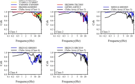
Coh k , computed by transferring Coh f in Figure 4-6 into the function of wavenumber domain based on h of horizontal component of S-wave, are shown in Figure 9-11. As for the horizontal component of S-wave, comparing between Figure 4 and 9, we can find that all Coh k in the same distance class get closer. Also, all Coh k decrease rapidly at about 0.5 wavenumbers, regardless of the distance classes. This indicates that subsurface soil at the depth of 0.5 wavelengths has strong effect on spatial variability of ground motion at adjacent observation sites.

The same trend can be seen in the vertical component of S and P-wave as the horizontal component of S-wave, but there are some non-negligible differences between Coh k in the same distance class, e.g. Coh k between HKD090-TKCH05 and other pairs of observation sites in the distance class 2 and Coh k between HKD142-SBSH03 and Chiba Array in the distance class 4.

Figure 9. S-wave Coherence of Horizontal Component by Distance Classes (Wavenumber Domain)

HKD142-SBSH03

(9)

Figure 10. S-wave Coherence of Vertical Component by Distance Classes (Wavenumber Domain)

Figure 11. P-wave Coherence of Vertical Component by Distance Classes (Wavenumber Domain)

HKD142-SBSH03

Chiba Array (Class 4) HKD123-SRCH10 Chiba Array (Class 5)

HKD142-SBSH03

(10)

CONCLUSION

The spatial variability of ground motion between adjacent observation sites are examined by analysing coherence Coh f of ground motion records obtained from the Chiba array and pairs of the K-NET and the KiK-net seismic network in Japan, which are adjacent to each other. It is found that Coh f strongly depends on subsurface soil structure and low P and S-wave velocity of subsurface soil causes a reduction of Coh f . We also found that the longer the distance between observation sites, the subsurface soil depth that effects to the spatial variability of ground motions h gets deeper, and Coh k rapidly decreases at the frequency which is equivalent to 0.5 wavenumbers to h .

ACKNOWLEDGEMENTS

We would like to thank for using the ground motion records of K-NET and KiK-net by the National Research Institute for Earth Science and Disaster Prevention, Japan and the Chiba Alley, University of Tokyo, provided by the Association for Earthquake Disaster Prevention, Japan. GMT is used to draw some of the figures.

REFERENCES

Abrahamson N. A. (2006), Program on Technology Innovation: Spatial Coherency Models for Soil-Structure Interaction, EPRI, Palo Alto, CA, and U. S. Department of Energy, Washington, DC: 2006.1012968

Association for Earthquake Disaster Prevention, Strong Motion Array Record Database, Vol.A02, Vol.A03, Vol.A05 (CD-ROM)

Chiu Hung-Chie, Amirbekian R. V., Bolt B. A. (1995), Transferability of Strong Ground-Motion Coherency between the SMART1 and SMART2 Arrays, Bulletin of the Seismological Society of America, Vol.85, No. 1, pp.342-348

Hao H., Oliveira C.S., Penzien J. (1989), Multiple-Station Ground Motion Processing and Simulation Based on SMART-1 Array Data, Nuclear Engineering and Design, Vol.111, pp.293-310

Harichandran R. S., Vanmarcke E.H. (1986), Stochastic Variation of Earthquake Ground Motion in Space and Time, Journal of Engineering Mechanics, Vol.112, No.2, pp.154-174

Katayama. T, Yamazaki. F, Nagata S., Satoh N. (1990), Earthquake observation by a three-dimensional seismometer array and its strong motion database, Journal of Japan Society of Civil Engineers, No.422, pp.361-369

Luco J. E., Wong H. L. (1986), Response of a Rigid Foundation to a Spatially Random Ground Motion, Earthquake Engineering and Structural Dynamics, Vol.14, pp.891-908

Nakamura H., Yamazaki F. (1995), Spatial Correlation of Earthquake Ground Motion Based on Dense Array Records, Journal of Japan Society of Civil Engineers, No.519, pp.185-197

National Research Institute for Earth Science and Disaster Resilience, Strong motion seismic networks, http://www.kyoshin.bosai.go.jp/kyoshin/

Schneider J. F., Stepp J. C., Abrahamson N. A. (1992), The spatial variation of earthquake ground motion and effects of local site conditions, Earthquake Engineering, 10th World Conference, pp.967-972