Speech Recognition Co-processor

(1)

CHANDRA, DHRUBA. Speech Recognition Co-processor. (Under the direction of Professor Paul D. Franzon.)

With computing trend moving towards ubiquitous computing propelled by the

advances in embedded mobile processors and battery technoloqy, speech recognition

is becoming an essential part of embedded processor I/O device. Speech recognition is

also used in command and control and automated customer service. Real time speech

recognition application is both computation and memory intensive and it overwhelms

even a high end multi-gigahertz processor to achieve real time performance. An

embedded mobile device cannot support real time large vocabulary speech recognition

application as the processors are less aggressive because of tighter power budget.

Hardware solution to speech recognition, in the past, have mainly concentrated on

building specialized hardware or ASIC accelerators to run software speech application

faster but have largely ignored design for large vocabulary and power reduction.

In this work, we propose a hardware-software co-design for real time large

vocabu-lary speech recognition. Our design has custom ASIC blocks and RAM memories and

a low power processor. The processor maintains a high level control over the blocks

and processes parts of speech recognition application which is not computation and

memory intensive. The custom ASIC computes the Gaussian probability and

per-forms word search in the dictionary. The RAMs are used for storing the intermediate

values and states. The design can handle large vocabulary speech recognition in real

time on a mobile embedded device. Our word search uses innovative dictionary word

layout in memory which reduces bandwidth by a factor of 11 compared to software

implementation and by a factor of 4 compared to other ASIC implementation. One

unit of our proposed design can perform 4x and 20x better than other proposed

de-sign of specialized hardware dede-sign for software speech application in computing the

(2)

by

Dhruba Chandra

A dissertation submitted to the Graduate Faculty of North Carolina State University

in partial fulfillment of the requirements for the Degree of

Doctor of Philosophy

Computer Engineering

Raleigh, North Carolina

2007

Approved By:

Dr. E. Rotenberg Dr. Robert Rodman

(3)

Dedication

(4)

Biography

Dhruba Chandra was born and raised in Durgapur, West Bengal, India. He received

a Bachelors and a Masters in Mathematics from Indian Institute of Technology (IIT),

Kharagpur. Dhruba joined graduate program in Applied Mathematics at North

Car-olina State University in fall of 1999. He received a Masters in Applied Mathematics

in fall of 2001 and a Masters in Computer Engineering in spring of 2002. Since spring

of 2003 he has been enrolled in computer engineering doctoral program at North

(5)

Acknowledgements

First and foremost, I would like to thank my advisor, Dr. Paul Franzon. His has

unique way of advising students. He encourages free thinking and his valuable

feed-back keeps his students on track and always motivated. He has always impressed

me and all other ECE graduate and undergradute students with his teaching. I am

thankful to all my committee members. I would like to thank Dr. Rhett Davis for

his valuable suggestions and for asking the critical questions. I thank Dr. Rotenberg

for teaching computer architecture courses and letting me use the modified

simplas-calar simulator. I thank Dr. John Wilson and Dr. Steve Lipa for always helping the

research group. I would like to thank my previous research group - Dr Solihin, Dr

Seong beom Kim, Dr Mazen Kharbutli and Fei Guo.

I thank my parents for their love, support and constant encouragement. My sister

has always been source of my inspiration. I would like to thank all my friends from my

undergraduate days - Bibhudatta Sahoo, Chandrasekhar Puthilathe, Debasis Mishra,

Mukul Khandelia, Ranadeb Chaudhuri, Shailendra Jha, Sunil Saini, Vinit Srivastava

Vivek Gulati, Saurav Prasad, Sumon Chattopadhye, Rohith S., Shubhadip Niyogi,

Pratik Chaudhury and Chandramauli Sastry. Thanks to Vikram Pendharkar, Paul

Palathingal, Jaishankar, Sajid, Tanvir, Milind, Shamsheer, Udayan, and Shashank

for friendship and tolerating me as their roommate. Thanks to the Volleyball gang

and Kausar Hassan.

(6)

of gallon of Java sipped, camaraderie I developed with the fellow coffee drinkers

and hundreds of hours invested - discussing world politics, NFL, college basketball

and research. Thanks to Cup-A-Joe for being that coffee shop. Thanks to Ajit

Rajagopal, Meeta Yadav, Nikola Vouk, Radha Venkatagiri, Salil Pant, Sarat

Kocher-lakota, Saurabh Sharma, Sibin Mohan, Surendra Jain for being the comrades. Time

spent with these folks in - Lab / Coffee Shop/ Glenwood South- is priceless. Thanks

to Nagendra Kumar and Milind Nemlekar for starting the evening coffee tradition.

I would like to thank my friend Ravi Jenkal for his help in my research. Thanks to

Ambarish Sule and Vimal Reddy for helping me in my research work with various

tools and simulator. Thanks to Meeta again for helping me in getting post defense

formalities done.

To all friends and folks in Raleigh, thank you for making my stay enjoyable over

(7)

List of Figures

1.1 Sphinx-III Performance [27] . . . 3

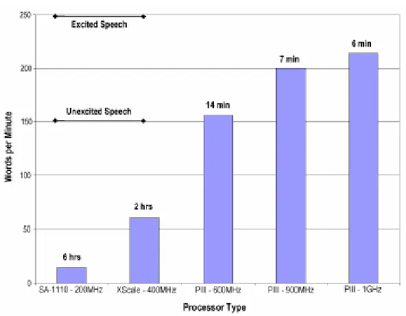
1.2 Battery Life-Words/min vs.Processor [24] . . . 4

1.3 Dictionary Word, Basic Sounds and Statistical Models . . . 6

1.4 Speech Recognition (Functional Blocks) . . . 7

1.5 Comparison Computation Performance . . . 9

1.6 Word search block Computation Performance . . . 9

2.1 Hidden Markov Model Experiment . . . 17

2.2 Composite HMM representing the word this ( th-ih-s ) . . . 19

2.3 Tied mixtures or Senones . . . 20

2.4 Dictionary Arrangements . . . 20

3.1 Frontend L1 Cache Miss Rate . . . 29

3.2 Frontend L2 Cache Miss Rate . . . 30

3.3 L1 Cache Miss Rate for Observation Probability Calculation . . . 30

(11)

3.5 L2 Miss Rate for Observation Probability Computation (2000 Senones) 32

3.8 Performance of Observation Probability on 1GHz Processor . . . 33

3.9 Triphone Evaluation Example . . . 34

3.10 Miss Rate for All Fresh nodes, and All Repeat Nodes . . . 36

3.11 Performance of Word Search Stage - Triphones per Frame . . . 37

3.12 Processing of Input Speech Pipelined across three Functional Blocks . 38 5.1 Speech Recognition System . . . 46

5.2 Speech Recognition Frontend . . . 49

5.3 Senone Evaluation and Word Decode Stage for first couple of frames 51 5.4 Observation Probability (OP) Unit . . . 54

5.5 Senone Score Memory . . . 55

5.6 Senone State Memory and Prioritizer . . . 57

5.7 Viterbi Decoder (δ = Delta) . . . 59

5.8 Triphone Representation using Senone ID . . . 60

5.9 Word and Lexical Tree information packed in a triphone packet . . . 61

5.10 Unfurled Flat Dictionary in RAM . . . 62

5.11 Triphone data block in Dictionary RAM . . . 63

5.12 Word Search Mechanism . . . 65

(12)

6.1 Bandwidth Comparison Senone Evaluation . . . 76

(13)

List of Tables

1.1 Cache size Miss-rate and Bandwidth . . . 5

6.1 Phoneme arcs and Active arcs in 12306 word Lexical Tree Dictionary 71

6.2 Power and Area of the Observation Probability Unit (0.18µ Tech) . . 73

6.3 Power and Area of the Word Decode Stage (0.18µTech) . . . 73

6.4 Performance per Senone and Senones Evaluated Per Frame . . . 76

6.5 Performance per Triphone and Triphones Evaluated Per Frame . . . . 77

6.6 Comparison of Power Consumption - Senone evaluation . . . 78

(14)

Introduction

1.1 Speech Recognition: Demand and Challenges

The advances in computing ability of processors, low power embedded processors

and artificial intelligence are making Human-Computer Interaction (HCI) and

ubiq-uitous computing a reality. Automatic speech recognition is an essential part of HCI

and ubiquitous computing and has some attractive advantages when used as an I/O

device for a system. Usually, a person can speak faster than he/she can type and it

keeps his/her other senses free to do other tasks.

Automatic speech recognition is also useful in applications like automated

cus-tomer service, interactive video games, and for controlling unmanned vehicle. With

the advent of battery operated mobile devices like cell-phone, PDA, speech

(15)

medical transcription etc. as the I/O (alphabet keyboard) of these battery operated

mobile devices are not user friendly. Automatic speech recognition coupled with an

automatic language translator can be used as language-to-language translation for

tourism, business or military purposes.

Speech recognition can done with template matching [6] but has limitations on its

usability. Any word spoken outside the pre-recorded templates are not recognizable.

Also, recognition may be speaker’s accent dependent. We now look at desirable/ideal

characteristic of a speech recognition system. A speech recognition system should

be as accurate as possible. Speech is different from the other I/O devices, such as

a computer key board, since in most cases it needs to be speaker independent. For

example, an automated customer service application may have callers with different

accents. Speaker independent speech recognition cannot be done using template

matching and is best handled using Hidden Markov Model (HMM), explained later

in the text.

When used as an I/O (speech to text) for emails, making documents or for

med-ical transcription the vocabulary needs to be fairly large since an ideal recognizer

should identify all words spoken, which may span the entire language dictionary. The

recognition should be done real-time/finite-time as otherwise the recognized speech

may lose its significance. Therefore, an ideal speech recognition system should be

a high accuracy real-time speaker independent Large Vocabulary Automatic Speech

(16)

different dialects.

Research in academia and industry have long pursued and developed high

accu-racy LVASR. The popular commercial systems available in market today are Dragon

naturally speaking [38], IBM’s Via Voice [4], Phillips-Freespeech98 [5] etc and systems

developed by academia are CMU-Sphinx [1], Cambrige-HTK [2] etc. These systems

are all software solutions, available as software packages and are run on desktop/server

platforms.

Speech recognition involves complex mathematical calculations involving floating

point numbers and has large memory requirement. Software solutions for speech

overwhelm a powerful desktop/server system because of their computational needs,

large memory and high memory bandwidth requirement.

(17)

Figure 1.2: Battery Life-Words/min vs.Processor [24]

Sphinx-III developed by CMU runs 1.8x slower than real-time on a 1.7 GHz AMD

Athelon [27]. The Figure 1.1 shows the processor speed and the recognition

perfor-mance for 29.3 sec of speech. In theory 1

, 2.4GHz is required to achieve real-time

performance. These recognition systems are memory intensive, have large memory

footprint, high L2 miss-rate and memory bandwidth requirement. The miss-rate of

L2 cache and bandwidth requirement are shown in Table 1.1. The recognition

sys-tem uses key resources of a syssys-tem (execution units, caches, bus bandwidth) because

of its high computational needs and high miss-rates of speech recognition and other

applications running on the desktop/server system may freeze because of resource

starvation. Moreover speech recognition is not scalable with processor frequency and

1

(18)

architectural changes are required. Figure 1.1 shows the battery life of two ’AA’

batteries if they power different processors running speech application.

Table 1.1: Cache size Miss-rate and Bandwidth

L2 Cache Size 2MB 4MB 8MB Miss Rate (%) 34.39 29.42 17.9 Bandwidth (MB/s) 1502 1261 773

It implies that the speech recognition application cannot be ported to battery

operated mobile devices as embedded processors (SA-1110 or X-scale) do not have

the required processing power and it is impractical to have a a Pentium / Athlon like

processor on a mobile device as it cannot be powered by a battery.

To make real time speech recognition work on embedded mobile enviroment, we

propose a system with a general purpose microprocessor, dedicated ASICs and RAMs.

We identify the computationally heavy and memory intensive parts of the speech

recognition and provide a solution with dedicated ASIC and RAM structures,

respec-tively. The microprocessor maintains a high-level control over the ASIC blocks and

performs computationally non-intensive tasks of the speech recognition.

We now take a look at speech recognition in somewhat more details 2

to quickly

identify the critical parts that cuases performance bottleneck (computationally heavy

and memory intensive parts) and solution proposed (key contributions).

2

(19)

1.1.1 Recognition Basics

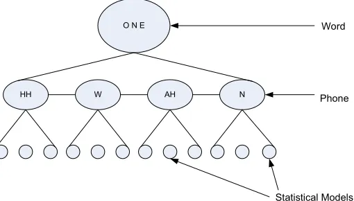
Any words spoken in a language is composed of a sequence of basic sounds. Sound

features of these basic sounds are captured and are represented as a collection of

multi-dimensional statistical models. The following figure 1.3 shows the word ”ONE” as

sequence of basic sounds ”HH-W-AH-N”. These basic sounds are also called phones. All words in a language dictionary are sequence of basic sounds.

Figure 1.3: Dictionary Word, Basic Sounds and Statistical Models

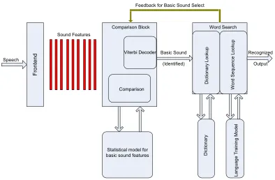
The following Figure 1.4 shows how a speech recognition system works. It is

divided in three broad functional blocks. Spoken words goes through Digital Signal

Processing (DSP) Frontend and sound features of the speech are extracted. To have a real-time recognition features are extracted every 10ms. These features are then

probabilistically compared with the huge database of all possible known basic sound

features to identify the most likely spoken sequence of sounds. (This database is

a collection of statistical models of basic sound features and is created by speech

(20)

of the dictionary words are mapped as sequence of sounds, the first part of the word

search block identifies the word(s) from dictionary.

! " # $% &

Figure 1.4: Speech Recognition (Functional Blocks)

There are many close sounding words and many different words may sound

sim-ilar because of speaker’s accent. It often happens that sequence of sound produced

matches closely with more than one word in the dictionary for one word spoken at the

frontend. All the close matching words are considered as poteintial candidate for the

actual word spoken. So a sentence with several words spoken at the frontend results

in a trellis of words identified as poteintial candidate for words spoken. The second

part (word sequence search) in word search block picks the most likely sequence of

words spoken from the trellis. This is done by baising certain sequences of words over

(21)

language training model.

1.1.2 Identifying Performance Bottlenecks

We now look at the performance bottlenecks in each block (as shown in Figure1.4)

of a speech recognition application run on a general purpose microprocessor. Our

speech recognition application is Sphinx-III [1]. We use Simplescalar [3]3

simulator for

the underlying processor architecture, is similar to present day application processor

on a mobile device. It is a 233MHz, 2-way out-of-order with 32KB L1 instruction

cache, 32KB L1 instruction cache, 256KB unified L2 cache (instruction and data).

Since the features are extracted every 10ms, we look at how the following parts

perform in processing the features extracted in 10ms. If each block takes 10ms or less

(i.e. 2.33 million cycles or less) in processing, a simple pipelined architecture with 3

stages would suffice.

The Frontend is a lightweight process and the software implementation for

ex-tracting features from speech signal take less than 1% [27,24] of the execution time

of speech recognition application on a general purpose microprocessor.

In the comparison block, there may be as many as 6000 (or more) different

sta-tistical models representing basic sound features. The number of comparisons can be

reduced with a feedback mechanism from the word search block. Figure 1.5 shows

the performance of the comparison part of the comparison block. Even one thousand

comparison takes around 16 million processor cycles. Usually, with feedback, the

3

(22)

Performance (Comparison block)

0 20 40 60 80 100

1K 2K 3K 4K 5K 6K # of c om pa ris on s Million Cycles

Figure 1.5: Comparison Computation Performance

number of comparisons reduced to around two thousand. All comparisons must be

done without feedback. Therefore, the comparisons are a bottleneck for a real time

speech recognition.

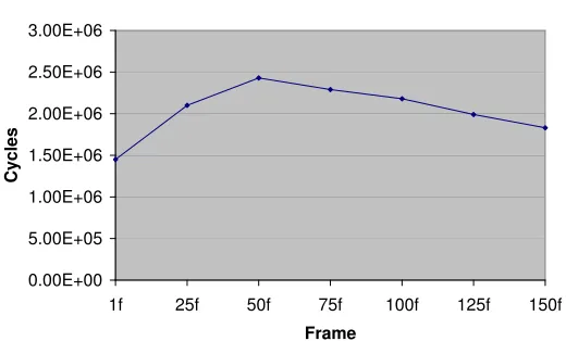
Performance - Word Search Block

0.00E+00 5.00E+05 1.00E+06 1.50E+06 2.00E+06 2.50E+06 3.00E+06

1f 25f 50f 75f 100f 125f 150f

Frame

C

yc

le

s

Figure 1.6: Word search block Computation Performance

We now look at the performance of word search functional block (Figure 1.6).

The performance of this functional block is dependent on size of the vocabulary. We

(23)

number of cycles needed for real time recognition for many frames. A dictionary for

large vocabulary is usually consists of hundred-thousand words. With those many

words in the dictionary, the number of frames not processed within 10ms is much more

than the number shown in the figure. Therefore, this gives us another bottleneck that

needs to be considered.

The performance of speech application clearly shows that real time recognition

is not possible on a present day embedded processor. In this work, we propose a

software-hardware co-design of the speech recognition system such that real time

recognition can be handled on a mobile device.

1.2 Proposed Solution and Key Contributions

• We propose a new design to traverse through lexical tree dictionary in hardware

and suggest an ASIC for word search, which uses this hardware tree traversal

to look through the words in the dictionary. It recognizes individual words and

provide information for determining the possible word sequences in the input

speech. One unit of this design performs about 20 times better than other

implementation of specialized hardware design to run speech application.

• Large vocabulary may have more than hundred thousand dictionary words. The

dictionary is stored in a DRAM memory. We propose a new way to store the

dictionary words in the DRAM which facilitates lexical tree traversal and

(24)

application and by a factor of 4 when compared to other hardware

implemen-tation of speech recognition.

• In the previous section, we saw that the comparison of a feature vector with

the database is a performance bottleneck. The comparison involves complicated

floating point calculations. We propose a dedicated ASIC for these

computa-tions. The ASIC can perform the required number of comparison within 10ms

(i.e. meets real time goal) and can operate in much lower frequency than the

processor, therefore saves power. This solution also enables the system to do

more exhaustive search and computation than a software speech recognition

ap-plication tailored for embedded enviroment. The design is flexible to algorithmic

changes in speech recognition theory which reduces processing requirement and

bandwidth, thus gives opportunity to reduce frequency and hence reduce power.

One ASIC unit performs 4 times better than one unit of specialized hardware

(processing element) for running speech application. The ASIC power

consump-tion is lower by a factor of eight.

• The feedback from the word search enables the comparison block to make

smaller number of relevant comparison in the database than comparing the

entire database. We design a mechanism which implements the feedback using

three small embedded SRAMs (1KB each). This design also priortizes some

(25)

1.3 Dissertation Outline

The remainder of the dissertation is organized as follows:

• Chapter 2 introduces the HMM based speech recognition theory in detail. The

Markov process is explained with a simple example of weather forcasting. The

hidden Markov model is introduced with the coin tossing example. Basic

defi-nitions and and an understanding of speech recognition system is presented.

• In chapter 3, we take look at the characteristics of speech recognition

applica-tions. Various performance bottlenecks are analyzed in greater detail, which

leads to our software - hardware co-design of the speech recognition system.

• Chapter 4 touches upons the related work in academia and industry. The

CMU-Sphinx system (opensource) is explained in detail as we use CMU-Sphinx system for

speech recognition Frontend and SphinxTrain for creating Acoustic and Lan-guage Models. Known speech recognition implementations in hardware is then

discussed.

• Chapter 5, presents our design, its various components and an understanding

of how the system works.

• Chapter 6 presents the performance and power results of our system and

com-pares it with the other related work.

(26)

Chapter 2 Hidden Markov Model and Speech

Recognition Theory

As mentioned earlier, speech recognition is usually efficient and accurate using

Hidden Markov Model (HMM). We start by understanding Markov process (chain)

and a hidden Model model and its application to speech recognition.

2.1 Markov Process

A Markov process is a stochastic process with Markov property. The Markov

property states that conditional probability of appearance of future state of a process,

given the present and all the past states only depends on the present state and not

on any of the past states. In other words, the future state is independent of the

path of the process (past states of the process). If X1, X2, X3, ..., XN are the random

variables which represents the occurrence of states s1, s2, s3, ...., sM then

P(Xi/Xi−1

(27)

where Xi−1

= Xi−1, ...., X3, X2, X1, i < N and the random variable Xi and Xi−1

represent the occurrence of state sp and sq, where p, q[1, M] respectively. The

prob-ability P(Xi = sp/Xi−1 =sq) is called the transition probability between the states

p and q and is represented by apq. The other properties associated with Markov

proccess are

M X

j=1

aij = 1; (2.2)

M X

j=1

P(X1 =sj) = 1; (2.3)

Both the equations represent basic principles of probablity theory that the sum of the

transition probabilities from one state to all of its possible next state is one and the

sum of the probabilities of the initial state being in any one of the M states is also

one. The Markov process above is called an observable Markov model. The output

of the process is a set of states, the occurence of each of which corresponds to an

event represented by the random variables. There is a one-to-one mapping between

observable event sequence X and Markov chain state sequence S.

The following example gives a good understanding of the Markov process and its

applicability. The summer weather in Raleigh, NC can be considered to have the

following three states.

• Really hot and dry (s1)

• Really hot and little humid (s2)

(28)

Let P(si) represent the probability of a certain day (initial day) being in state si.

Since the summer days are categorized into the above three states, any particular day

will be either dry or little humid or very humid. Therefore, probability that the intial

day is either dry, little humid or very humid (equaton 2.3) follows:

P(s1) +P(s2) +P(s3) = 1; (2.4)

Assume,P(s1) = 0.4,P(s2) = 0.4 andP(s3) = 0.3. Now, if the transition probability

from dry, little or very humid weather on a particular day to dry(d), little humid(l.h)

or very humid(v.h) next day is given by the following matrix:

aij =

d l.h v.h

d l.h v.h        

0.2 0.6 0.2

0.3 0.3 0.4

0.1 0.3 0.6

       

The above matrix is called transition probability matrix for this system. The

sum-ming transition probabilities to all possible weather states for next days we get one

(equation 2.2). In above probability transition matrix this corresponds to the sum

of the row elements. With above information we can forecast the probability of a

particular weather pattern using Markov process. Probability of a weather pattern

−l.h₋> d₋> l.h₋> v.h₋> l.h₋> d₋> v.h₋> v.h₋ is evaluated as follows:

P(O_|M) = P(s2, s1, s2, s3, s2, s1, s3, s3)

(29)

= (0.4)(0.3)(0.6)(0.4)(0.3)(0.3)(0.1)(0.6)

= 0.00015552

2.2 Hidden Markov Model

The above Markov model is observable, i.e states are observed when an event oc-curs. This observable Markov model is too restrictive and cannot be applied to many

problems. Alternately, Markov model can be extended such that the observations are

probabilistic functions of the state. In other words, it is a double-embedded stochastic

process with an underlying stochastic process not directly observable (hidden). This

underlying stochastic process can only be probabilistically associated with another

observable stochastic process producing the sequence of features we can observe. The

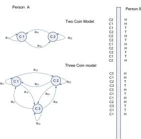
hidden Markov model concept is well understood through the well known coin toss

example [34]. Assume that there is a coin tossing experiment where a person (say

person A) is performing coin tosses from two different sets of coins: one set has two

coins in it and the other one has three coins in it. Person A can select any coin from

just one set for the toss. Now another person (say person B) can’t see howA chooses

a coin but just observes the outcome of sequence of head and tail.

The observation O is sequence of head or tail tossed by person A and seen by

person B. Each set can produce an observation and each individual coin can be

(30)

Figure 2.1: Hidden Markov Model Experiment

will be tossed is the transition probabilityaij (thejth _{coin will be tossed immediately}

after the ith_{). The person} _B _{can now probabilistically determine whether the two}

coin model or the three coin model was most likely used for tossing.

HMM based speech recognition uses the same concept. Any utterence (speech)

is composed of sequence of basic sounds. Any word in dictionary is composed of

se-quence of basic sounds. Each of these basic sound have statistical models. Therefore,

a word can be expressed as sequence of statistical models. Speech (to be recognized)

is sampled by the the speech recognition system to form a sequence of speech feature

vectors (numerical parameters). This sequence of speech feature vector is the

(31)

most likely would produced the speech vector. Identifying the model sequence results

in identifying the word spoken.

2.3 Speech Recognition Theory

A spoken word or phrase is represented as a sequence of basic sounds called phone or phoneme [39, 18, 20, 15]. For example, there are approximately 51 phonemes in the English language. A Permutation of these phones leads to a word or a phrase.

The sentence ”This is speech” is phonetically broken down to ’th ih s ih z s p iy sh’.

Phones are an excellent means for encoding word pronunciation but they are not

ideal for recognition of speech. The contextual affects cause variation in the way the

basic sounds are produced. Each of the phones along with it neighboring phones (left

and right) is called a triphone. Therefore, in above example sound of ’ih’ is effected by neighboring ’th’ (left phone) and ’s’ (right phone). Recognizing triphone units in

context tends to be more accurate than recognizing individual phones. The triphones

are represented with a ’-/+’ sign so ’th-ih+s’ represent a triphone where ’th’ and ’s’

are the left and right phones respectively. The first phone in any utterance has ’sil’

(representing silence) as the left phone. The total number of possible triphones in

English is around 65000. The phones without any influencing neighbouring phones

are called context-independent phones. In this text, phones and triphones are used interchangeably. Context-indenpendent phone refers to original phone without any

(32)

Y Z P

X Q Y R U U

Th ih s

Figure 2.2: Composite HMM representing the word this ( th-ih-s )

In HMM based speech recognition theory, for each phone and triphone, there is

a corresponding statistical model called hidden Markov model. These HMMs are

sequence of states called Markov states, connected by probabilistic transitions. Each

of these states have one or more entry and exit states. Exit state of one triphone

merged to entry state of another forms composite HMM, which allows to represent a word and then the words joined together to form a phrase or utterance.

Figure2.2is an example1

of a three state HMM representing the word ”this”. The

states in triphones are best represented by multi-variate mixture Gaussian

distribu-tion. The parameters for the statistical models which represents the states (Gaussian

mixtures and transition probabilities) are obtained from the training data and is

collectively called the Acoustic Model.

In absence of sufficient training data or to avoid redundancy of data the states

of different triphones can be sometimes represented by same distribution [21, 40],

and these are called senones or tied mixtures. Therefore, a combination of senones 1

(33)

Figure 2.3: Tied mixtures or Senones

forms triphones, which, in turn, combine to form words and words, themselves, come

together to form a sentence or an utterance. Number of senones in English language

is around 6000.

The collection of all words is called the dictionary. The dictionary words are phonetically broken down and are stored in eitherflatform orlexical treeform [14,36]. Figure 2.4 shows two form of dictionary arrangement representing words - Start,

Starting, Started and Startup.

S S S S T T T T AA AA AA AA AA R TD DX DX DX IX IX PD DD NG T

R AX

R T PD DD NG AX IX IX DX DX R R TD

R T

S

FLAT LEXICAL TREE

(34)

In a speech recognition, speech or the utterance (to be recognized) is a sequence of

words. It goes through theFrontend, where spectral analysis is done to extract the fea-ture vectors(input acoustic vectors). These feature vectors are sampled at fixed inter-vals (10 ms). The sequence of vectors thus obtained is called theobservation sequence . If the observation sequence is O=O1, O2, O3, ..., OT, where Oi represents a feature

vector sampled at fixed interval, the speech recognition decoder (the decoder is the

part which does the actual recognition) finds the sequence of words (i.e. sequence

phones or triphones) which is most likely to produce the observation O. If the

se-quence of n words is represented by W =W1, W2, W3...., Wn, the decoder maximizes

P(W_|O), whereP represents the probability. We want to maximize P(W_|O),

apply-ing Bayes’ theorem

P(W) =argWmaxP(W_|O) =argWmaxP(W).P(O|W)

P(O) (2.5)

Where P(W) represents the probability of a word sequence and is available from

language model. P(O) is the probability of the observation sequence. P(O_|W) is the

probability of observation sequence O, given the word sequence W. It is computed

using a composite hidden Markov model forW, constructed from simple HMM phone

or triphone models joined in sequence (according to word pronunciations stored in a

dictionary).

In speech recognition, HMM generates speech feature vector sequences. It is a

finite state machine which changes state every time unit and each time t that a

(35)

called the observation probability. As mentioned earlier, each of the transition is probabilistic. The probability of transition from statei to statej is given by discrete

probability, called the transition probability and is represented by aij.

The joint probability of observation of vector sequence O and state sequence

X = xo, x1, x2...xT−1, given some model M is calculated as product of the

transi-tion probabilities and the output probabilities.

P(O, X_|M) = b0(O0)ΠT−1

t=1 bxt(Ot)axt−1xt (2.6)

assuming the HMM is in state 0 at timet= 0. In practice, only observation sequence

O is known and underlying state sequence is hidden. The probability P(O_|M) is

determined by the probability associated with the state sequence which maximizes

P(O, X_|M). This is calculated usingViterbi decoder. We defineδt(j) as the maximum probability that the HMM is in state j at time t. The value δt(j) is computed, as

follows

δt(j) =max0≤i≤N−1[δt−1(i)aij].bj(Ot) (2.7)

where i is the previous state (at time t₋ 1). The observation probability bj(Ot),

where Ot represents the probability that state j emits observation feature vector

Ot for observation sequence number t. The observation probability [40] is mixture

multivariate Gaussian distribution is given by

bj(Ot) =

M X

m=1

(36)

where cjm is the weight of the mixture component, m in statej and N(Ot;µjm, σjm)

is the multivariate Gaussian with meanµ and covariance σ

N(Ot;µj, σj) = (_√_L1 2π)

1

p

Πσji.e

−1₂P(Oji−µji)2 2σ2

ji (2.9)

Lis the dimension of the feature vector considered (summation and multiplication

is done from 1 through L). Calculation of observation probability is computationally

very intensive and is usually calculated in logarithm domain to reduce the complexity.

Moreover, it is calculated against large number of senones per frame.

2.4 Language Model

The language model is used by large vocabulary speech recognition system to

increase recognition accuracy [8, 9, 31]. It helps in identifying the most probable

sequence of words uttered from a large pool of words recognized as candidate for

ac-tual words spoken. The Language model selects a sequence of words attaching more

weight to certain word sequence out of pool of alternative word sequences produced

by the acoustic model for possible match. Weight are priori probability of sequence of

words. Inclusion of language model also helps in increasing efficiency of speech

recog-nition system by eliminating (pruning) the unlikely path for word sequence search.

All the present day speech recognition systems have some sort of language model.

The language model also enables the recognition system to have correct syntax and

semantics of the language. It helps in forming meaningful and grammatically well

(37)

theory [29] 2

or by using probabilistic language model (Stochastic language model).

Most of the recognition system uses Stochastic Language Model (SLM) [23].

2.4.1 Stochastic Language Models

Stochastic language modeling is a probabilistic approach to language modeling.

The most commonly used SLM is the N-gram model. It provides adequate

proba-bilistic information so that likely word sequence has the maximum probability among

all other possible word sequence.

N-gram Models

Revisiting equation 2.5, P(W) is the probability of word sequence. P(W) is

mathematically expressed in the following form.

P(W) = P(w1, w2, w3, ..., wn)

= P(w1)P(w2_|w1)P(w3_|w1, w2)...P(wn_|w1, w2, w3, ...wn−1)

= Πn

i=1P(wi|w1, w2, ...wi−1) (2.10)

where P(wi) is the probability of wordwi appear following the occurence of word

sequence w1, w2, w3,...,wi−1. The probability evaluation is managable with small

vocabulary size since the complexity of the language model increases exponentially

with the vocabulary size. If the vocabulary size is V, the word wi will have Vi−1

histories and it is practically impossible to evaluate all the values even for a moderate

2

(38)

value of i. To reduce the complexity of the P(W) a variant of above probability

formulation is considered. Instead of P(wi_|w1, w2, w3...., wi−1) an equivalance class

P(wi_|wi−N+1, wi−N+2, wi−N+3...., wi−1) is considered. This is called the N-gram

lan-guage model [17, 33]. When N = 1 we have P(W) = ΠP(wi) - unigram language model, the probability ofith word does not depend upon any previously spoken words

but depends on probability of a word appearing in training data. When N = 2 we

have P(W) = ΠP(wi_|wi−1) - bigram language model. Therefore, bigram language

model suggests that probability of appearence of a word in an utterence depends on

the previous word uttered. When N = 3 we have P(W) = ΠP(wi_|wi−1, wi−2) -

tri-gramlanguage model - probability of word appearing in an utterence depends on two previous words uttered. The three language models listed above are most commonly

used in speech recognition systems. In some of the systems N = 5 is also used. The

probabilities of all these stochastic language models are predefined for speech

recog-nition process, and the values are obtained from training the language model using

training data. The probabilities for N-gram(N = 3) model are usually calculated

using the following formula.

P(wi_|wi−1, wi−2) =

F(wi−2, wi−1, wi)

F(wi−2, wi−1)

(2.11)

F(wi−2, wi−1, wi) refers to the frequency of occurrence of the trigram (wi−2, wi−1, wi)

in the training text and F(wi−2, wi−1) refers to the frequency of occurrence of the

bi-gram (wi−2, wi−1). The training data however may not cover entire vocabulary or have

(39)

system using N-gram model may bias against a sequence of words which has

max-imum likelyhood according to acoustic model of the system. In such cases M-gram

(M < N) probabilities are used in the place of N-gram probabilities after reducing

the probability by a back-off weight which accounts for the fact that the next higher

N-gram has not been seen and therefore has a lower chance of occurring [12].

Alter-natively, smoothing technique is used to get the N-gram probabilitiies. In N-gram

smoothing, the low probabilities are raised and the high probabilities are lowered.

The idea is to keep the language model with extreme values (N-gram probability of 0

or 1)totally overriding the the selection of word sequence even though acoustic model

may suggest otherwise. A simple smoothing technique is to assume any trigram

(se-quence of three words) appears one more than actually observed in the training data

as shown below.

P(wi_|wi−1, wi−2) =

1 +F(wi−2, wi−1, wi)

P

wi(1 +F(wi−2, wi−1, wi))

(2.12)

With above equation2.12, the probability of any unseen trigram in the training data

(40)

Chapter 3 Evaluation and Analysis of Speech

Recognition Application

In this chapter, we look at how speech recognition application performs on a

gen-eral purpose microprocessor. Our goal is to achieve real time large vocabulary speech

recognition on a battery operated mobile device. We first evaluate the performance

of speech recognition software application in processing one frame of speech on a

gen-eral purpose microprocessor. One frame of speech is speech input in 10ms (sampling

interval). In order to have a real time recognition one frame of speech input must be

processed within 10ms or less.

We use Sphinx-III [1] for our evaluation and analysis. This is because, Sphinx is

open source, free and achieves good recognition (fast and low error rate). In chapter

1, we mention that the speech recognition has three major independent functional

parts - the Frontend, the Comparison Block (probability computation) and the Word

Search. We evaluate and analyze each of these parts separately. The performance

(41)

chap-ter 1, figure1.1and figure1.2, respectively. Our analysis based on different functional

parts, helps us understand various performance bottlenecks of the application when

run on a general purpose microprocessor. It also helps us decide, hardware software

partition in for a hardware-software system design for speech recognition.

Any speech recognition system implemented in software or hardware needs large

memory for the acoustic model, dictionary and language model storage. The acoustic

model is looked up numerous times every frame as senones are evaluated in each and

every frame in the recognition process. The dictionary is also looked up every frame

for the matching triphones. The language model is looked up less frequently than

the acoustic model and dictionary. For a software speech recognition application

on a general purpose microprocessor these memory lookups are converted to loads

and stores (generated because of storing various scores computed in the process of

recognition). In case of hardware (hardware accelerator) implementations the lookups

and stores are memory reads and writes.

3.1 Performance Analysis of the Functional Blocks

We saw a brief performance evaluation in chapter 1. We now present detailed

performance analysis of the functional blocks. Since speech recognition is very

mem-ory intensive, we present the complete analysis of the application’s memmem-ory behavior

(42)

3.1.1 Frontend

The Frontend converts the speech input to acoustic vectors. The speech signals

undergo digital signal processing and acoustic vectors [25, 26] are obtained. The

Frontend only counts for 1-2% of the processing time of speech recognition application

[24,27]. Though, Frontend is a light weight process (low processing time), we still look

at its memory characteristic since its memory behavior may effect the performance of

other jobs running simultaneously. The following figures 3.1 and 3.2 shows the miss

rates of the Frontend in L1 and L2 cache.

0 0.01 0.02 0.03 0.04 0.05

16K 32K 64K

Cache Size

M

is

s

R

at

e

Figure 3.1: Frontend L1 Cache Miss Rate

3.1.2 Observation Probability Computation

In chapter 1, we have seen the time taken to evaluate senone scores for different

number of senones. The amount of time taken to score a group of senones is linearly

(43)

0 0.05 0.1 0.15 0.2 0.25 0.3

64K 128K 256K 512K 1024K 2048K

Cache Size M is s R at e

Figure 3.2: Frontend L2 Cache Miss Rate

expected and is observed in Figure1.5. The reason for this linear trend is the fact that

the senone score (observation probability) is evaluated using equation 2.8 and each

senone has different acoustic parameters (mean, variance and constant cofficients).

The acoustic parameter for each senone is around 2.5KB. Once a senone score is

computed its 2.5KB of data is never reused. So N senones would require 2.5*N KB

of data. 0 0.005 0.01 0.015 0.02

8K 16K 32K 64K

L1 Cache Size

M is s R at e

2000 Senones 4000 Senones 6000 Senones

(44)

Figure 3.3, shows the L1 cache miss rates of the observation probability

calucula-tion of 2000, 4000 and 6000 senones on different cache sizes. Figure 3.4 shows ratio

of number of hits per way in L1 cache. The high hit rate in most recently used cache

line imply of a good spatial locality. The observation probability calculation is

ex-pected to show high spatial locality since each of the parameters in acoustic model is

4 byte (32 bits) wide and are packed together in cache blocks and each of the senone

is evaluated one by one.

0 0.1 0.2 0.3 0.4 0.5 0.6 0.7 0.8 0.9

MRU LRU MISS

L1 Ways R at io -L 1 A cc es se s)

2000 Senones 4000 Senones 6000 Senones

Figure 3.4: Access pattern in L1 Cache

The miss rate in L2 cache is shown in Figure3.5, 3.6and 3.7. The high miss rates

in L2 and the pattern of hits in the L1 ways indicate that lack of temporal locality

in data used to evaluate the observation probability of senones. The high number of

accesses to L2 cache with high miss rate results in cache pollution and effects other

application threads or different threads of the same application. It tends to increase

the number of misses in L2 access for other threads possibly slowing them down [10].

(45)

L2 Miss Rate (2000 Senone)

0.8 0.85 0.9 0.95 1

64K 128K 256K 512K 1024K 2048K

Cache Size

L1=16K L1=32K

Figure 3.5: L2 Miss Rate for Observation Probability Computation (2000 Senones)

L2 Miss Rate (4000 Senones)

0.8 0.85 0.9 0.95 1

64K 128K 256K 512K 1024K 2048K

Cache Size

L1=16K L1=32K

imply that observation probability of senone can be computed with one hierarchy of

small cache size.

We now focus on the computational part of the senone score evaluation. This is

done by assuming one cycle latency in all loads and stores,i.e., every memory request (including the cold misses) is assumed to be a hit in L1 cache. Figure 3.8 shows the

performance on senone computation in two different architecture platform for 2000

(46)

L2 Miss Rate (6000 Senones) 0.8 0.85 0.9 0.95 1

64K 128K 256K 512K 1024K 2048K

Cache Size

L1=16K L1=32K

processor.

Performance of Observation Probability Calculation

0 1 2 3 4 5 6 7 8 9 10

1K 2K 3K 4K 5K 6K

# of Senones

Fr am e in te rv al (1 0m s)

L1-L2-Memory No Memory Latency

Figure 3.8: Performance of Observation Probability on 1GHz Processor

Ideally, all senones in an acoustic model used in recognition system should be

scored within one frame. Therefore, for large vocabulary speech in English, having

1000 or more senones, real time recognition is not possible since it takes about 8.6

times more time to compute.

(47)

time requirement. Therefore, either architectural changes are needed for running the

speech application or ASIC accelerator is needed to to speed up the computation.

3.1.3 Word Search

The words in a speech recognition system are represented by sequence of triphones.

Each triphone is represented by three senone sequence in 3-state HMM (or five senone

sequence in 5-state HMM) and the transition matrix. If the senone scores are

avail-able, the triphone score can be computed using a Viterbi decoder [13, 16, 19, 22]. In

each frame, the word search computes its triphone scores. A triphone (in a word)

may be computed in consecutive frames, also one frame may compute more than one

triphone. (shown in figure 3.9).

Figure 3.9: Triphone Evaluation Example

A word is idtentified by the speech recognition system as spoken word when it

detects the last triphone of the word and the over all word score (sum of score of each

(48)

is above preassigned threshold. We refer triphones in a word as nodes or triphone nodes.

For real time speech recognition, every frame needs to evaluate certain number of

nodes. These nodes are called the active nodes. The number actives nodes changes dynamically based on algorithm implemented in the speech recognition system.

Dic-tionary used in the speech recognition application is a lexical tree dicDic-tionary where

the different words share the common nodes. Sharing reduces memory space for

stor-ing dictionary words and reduces redundant score computation. The computation of

each node with available input data takes same amount of time.

With the dictionary arranged in lexical tree format the two factors effecting the

performance of this stage are number of active nodes and memory latency of input

data. Unlike senone evaluation stage, the cache hierarchy plays an important role

in determining the performance of this stage. The reason for this is the fact that a

particular node may be active in two or more consecutive frames, therefore, a high

possibility of the node data structure being found in the cache. In presence of a node

data structure in cache hierarchy results in quicker score evaluation because of smaller

latency for data.

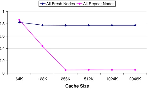
There are three possible categories in which we can classify the performance of the

word search stage. They are 1) None or very few active nodes present in the cache

hierarchy (High miss mate 2) Almost all or majority of the active nodes present in

(49)

nor the misses (nodes not preset in the cache) on active nodes are ignorable. The

following figure (Fig. 3.10) shows first two categories. It shows the miss rates of the

L2 cache accesses by the word search in frame duration. All fresh nodes signifies

that score of each node is computed for the first time in this frame, therefore causing

L2 cache misses. Score of a node computed in the preceding frame is a repeat node

and likely to result in cache hits. The miss rates for the third category is bounded

within maximum and minimum miss rates values available for these curves. It is

L2 Miss Rate (Word Search)

0 0.2 0.4 0.6 0.8 1

64K 128K 256K 512K 1024K 2048K

Cache Size

All Fresh Nodes All Repeat Nodes

Figure 3.10: Miss Rate for All Fresh nodes, and All Repeat Nodes

difficult to estimate the performance of the word search part of speech recognition

application and guarantee real time performance since the number of active triphone

nodes and the repeat characteristic of the active triphones in consecutive frames are

input (speech) dependent. We, therefore, bound the performance of word search

between time taken to compute one triphone node score under cache hit and time

taken to compute one triphone node score under cache miss. The figure (Fig. 3.11)

(50)

10 ms). (These values are not linear with processor speed. The processor speed is

only used for calculation of processor memory latency in cycles)

0 1000 2000 3000 4000 5000 6000

233 MHz 400 MHz 1000 MHz

Processor Speed N um be r o f T rip ho ne s

All Fresh All Repeat (L1 Hits)

Figure 3.11: Performance of Word Search Stage - Triphones per Frame

3.2 Building a Case for our Design

We now find a solution for real time speech recognition. For real time speech

recognition, input speech is sampled every 10ms and must be processed within 10ms.

This involves processing by the Frontend, computing the observation probability and

processing by the Word Search block.

We have seen in the previous section that a very aggressive processor (1 GHZ,

2-way, 32KB L1D, 32KB L1I, 256KB L2) cannot process the computation of observation

probability even for 1000 senones within 10ms. Moreover, it can poteintially slow

down other applications or other parts of speech recognition application because of

its high miss rate in L2. Since the calculation of probability is same for all senones,

(51)

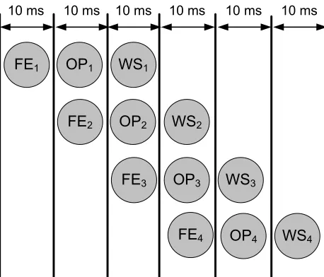
Figure 3.12: Processing of Input Speech Pipelined across three Functional Blocks

The performance of word search cannot be gauranteed since it depends on

avail-ability of cache hierarchy, size of the vocabulary (dictionary size) and input speech.

We suggest an ASIC for computation and a RAM for the dictionary to gaurantee

performance of based on number of triphones that can be processed.

We separate out the three functional blocks and compute each of these in parallel

as shown in the figure (Fig. 3.12). This give more time to each block to process.

ASIC blocks can operate on much lower clock frequency and perform much better

(52)

Chapter 4 Related Work

Speech recognition applications have been developed in industry for commercial

purpose as well as in university for academic interests. Most of the speech

recogni-tion systems are based on HMM. The software solurecogni-tions for speech recognirecogni-tion are

available as software packages. These packages have two parts - the decoder, which

does the actual recognition of the utterance and the acoustic and language models,

which are used by the decoder. The software solutions are efficient implementation

of speech recognition algorithms in high level language, therefore need a general

pur-pose microprocessor. The decoder is computationally very demanding and dedicated

hardware units and platforms have been built in academia and the industry. These

hardware approaches usually use the acoustic and language models of the software

packages. We now look at few software solutions as well as hardware approaches for

(53)

4.1 Software Solutions

The AT&T Watson speech recognition engine [35] is a software implementation

of AT&T voice processing technology. This system is HMM based and the uses

gender based triphone models. In 94 NAB 1

evaluation, the system has around 22000

context dependent phones. The language model is 5-gram. The recognition is in two

passes, the first pass does the phone recognition, word recognition and build the word

lattice and the second pass rescores the word graph. The system works on Pentium

with Win/NT operating system. This system also implemented for shared memory

multiprocessor architecture [32].

The IBM speech recognition is known as Via-Voice. It is different from other speech recognition system. It uses rank-based approach 2

for the computation of

ob-servation probabilities. The search technique is a combination of A* search 3

heuristic

and time synchronous Viterbi decoding. A version of Via-Voice designed for

embed-ded processors and works on PDA’s and automobile GPS system and mobile devices

for command and control. A detail on this version is not available in literature.

SRI international’s Speech Technology And Research (STAR) groups has speech

recognition system called DECIPHER. The system is HMM based and does

multi-pass time synchronous Viterbi decoding. The system uses tied-mixture states.

Sphinx-II speech recognition system was developed by CMU (later versions are

1

Benchmark 2

Not discussed in this report 3

(54)

III and IV). This system is based on hidden Markov models.

Sphinx-II uses normalized feature representation, multiple-codebook semi continuous hidden

Markov models [20]. It has multi-pass search architecture and unified acoustic and

language models. For the HMM states it uses senones based approach tying mixtures

of similar Gaussian distribution. It uses scaled-integer for computation of observation

probability. The multi-pass search architecture is mainly used when the vocabulary is

large. Viterbi algorithm is efficient but less optimal compared to A* search algorithm.

In first pass, Viterbi decoding is done to reduce the search space for A* algorithm. In

second pass the A* search combines the result of Viterbi decoding and the language

model to effectively do the recognition. Sphinx uses a unified stochastic engine which

combines acoustic model and the language model and jointly optimizes both the

models. The newer versions of Sphinx are built on the older version. The Sphinx-III

and Sphinx-IV uses lexical trees rather than flat dictionary. The searches in the higher

version are efficient using beam searchs and various pruning strategies. The acoustic

models consist of 3-state or 5-state HMMs. Sphinx is only good for academic interest

as it requires extraordinary memory and high-end workstation for speech recognition.

Microsoft Whisper is built on the basics of CMU-Sphinx system is more

appli-cable in real world. It works on common desktop machines. Whisper uses speaker

adaptation and noise cancellation. Whisper is memory efficient as the acoustic model

is compressed and has no decompression overhead effect on speech recognition and

(55)

Binu et.al. [27] worked on Sphinx-III and made it more efficient. They targeted

on reducing the bandwidth requirement for calculating observation probability. Since

observation probability for a single senone requires lot of data corresponding to the

mean, variance and the weight mixtures and the calculations are done every frame,

their scheme calculated probability of a senone for ten consecutive frames before

moving on to the next senone. This reduces the bandwidth requirement by ten times,

if all the senones are to be evaluated every frame. Moreover, calculating senone score

for ten consecutine frames leads to more cache hits therefore has better performances.

4.1.1 Problems with Software Solution

Before going into hardware solutions for speech recognition, we re-visit the

prob-lems software implementation has with HMM based speech recognition.

• The calculation is slow because of complicated mathematical operation even on high performance platform. (Floating point multiplication, logarithm

calcu-lation or exponent calcucalcu-lation)

• To have simplicity, fixed point or scaled-integer arithmetic is used instead of floating point, therefore it induces inaccuracy.

• To speed up recognition, number of computation is reduced by introducing

threshold values. This also induces inaccuracy.

• The computational need of speech recognition algorithm freezes most of the

(56)

• Speech Recognition requires large amount of memory (Table 1.1) for storing

the parameters of statistical model (example Mean, Variance, Weights etc),

language model and dictionary.

– It has large working set which causes problem when some other application runs on the same platform. They share the same cache hierarchy resulting

in contention and therefore affecting each others performance.

– The memory bandwidth requirement is a bottleneck.

• Software solution ispower hungry.

4.2 Hardware Solutions

Software solution fails to achieve the real time speech recognition, which is

accu-rate and has tight power budget needed for mobile devices. Hardware-software

ap-proaches have been tried by many researchers. Mainly hardware accelerators [27, 28]

for calculating the observation probability were implemented in academia. There are

several IC’s for speech recognition but it is not clear whether they do anything other

than the frontend DSP and the probability calculation.

Low power accelerator [27] implements the computation of observation

proba-bility. The design acts as accelerator for Sphinx-III speech recognition system. The

implementation has floating-point arithmetic. The floating point arithmetic, however,

is not same as the IEEE-754 standards, instead has only 12-bit mantissa. Smaller

(57)

buffers the feature vectors from ten consecutive frames and then evaluates the

acous-tic score (probability) with respect to each senone. This enhances the performance

with more cache hits (if there is a cache type fast memory buffer in the embedded

en-vironment) and reduced bandwidth requirement. This design (0.25µ process) shows

29-fold improvement in power consumption over the software implementations used

by Sphinx-III on Pentium-4 (0.13µ process). Though, this design optimizes

Sphinx-III for embedded environment, it evaluates senone score for ten consecutive frames

together, therefore restricting any algorithmic optimization using the Viterbi decoder

feedback. Other than computation of probability, the Viterbi algorithm for optimal

path and the search of optimal path in word lattice is computationally demanding and

therefore accelerator is not a complete solution for enhancing real-time performance.

Hardware implementation speech recognition system, with FPGA acting as a

co-processor [28] for speech recognition is an alternative to ASIC implementation of

real-time recognition. This implementation however, is not designed for power efficiency.

Low power device for speech recognitions implemented by Sergiu et.al. [30] does

real-time speech recognition. Unlike other hardware recognition systems which are

usually accelerators for certain function in the software, this design is a complete

recognition system. It has its own language and acoustic model. This

implementa-tion does not use the n-gram language model, instead uses regular grammar based

language model to ease the search space. It exploits parallelism existing in speech

(58)

helps in reducing clock frequency resulting in reduced power usage. The acoustic and

language models are kept in FLASH memory and SRAM is used for dynamic memory

required for intermidiate stages of recognition. The design however is good for a very

(59)

Chapter 5 System Architecture

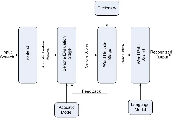
The speech recognition system that we design has components shown in Figure5.1.

The input speech goes through the Frontend, where spectral analysis is done to extract

acoustic feature vectors.

!

"

Figure 5.1: Speech Recognition System

These acoustic feature vectors then go through thesenone evaluation stage, where the observation probability of each senone is calculated. This probability is also called

(60)

easily (triphones are collection of senones) and is done by theword decode stage. This stage calculates the triphones scores of the dictionary words. Also, the word score is

calculated, summing all the triphone scores of the component triphones. The probable

spoken word is identified based on word scores. Over time, it generates a word lattice

over time. The word lattice is then evaluated by the Word Path Searchfor the most likely spoken word sequence in the input speech.

The word decode stage also provides the senone evaluation stage with information

about the relevant senones whose score must be evaluated in the next frame. This is

shown by ’Feedback’ in the figure.

As shown in the previous chapters, an acoustic vector is easily processed within

10ms and the native execution takes only 1% of the computation time. We, in our

system, have the Frontend in software which is run on the general purpose

micropro-cessor. Our design proposes ASIC and RAM structures for the senone evaluation and

word decode stages since the real time processing (of these two stages) is not possible

using a general purpose microprocessor.

We now give detail of the Frontend, then a brief understanding of how the senone

evaluation and the word decode works using ASIC blocks we design along with RAM

(61)

5.1 Frontend

The system audio device converts the spoken words into the speech signals. The

speech signals are sampled over an interval of few milliseconds. The spectral

charac-teristic of speech is assumed to be constant within the interval. Frontend takes the

sampled speech signals as input and generates the speech feature vectors as output.

It performs a spectral analysis of speech signals. It is assumed that the speech signals

correspond only and only to the spoken words on the audio device. i.e, all background

words/noise does not contribute to the speech signal. Linear Predictive Coding (LPC)

is used for the spectral analysis. We go through the brief detail of each of the steps

involved. Figure 5.2 shows the block diagram of a speech recognition frontend. The

overall block action is a frame ofN samples is processed and a speech feature vector

Ot is computed.

The intervals are typically spaced 10 msecs. Blocks are overlapped to give a

longer analysis window, typically 25 msecs. The raw signal is then pre-emphasized

by applying high frequency amplification to compensate for the radiation from the

lips.

Spectral estimates can be computed via linear prediction or discrete Fourier

anal-ysis or cepstrum analanal-ysis, and the coefficients, i.e., the final acoustic vectors can be obtained via a number of transformations. The most typical method of modern LVR

systems is to use the mel-frequency cepstral coefficients (MFCCs). The processing

(62)

Figure 5.2: Speech Recognition Frontend

The Fourier spectrum of each speech block is smoothed by a mel-scale filter-bank

that consists of 24 band-pass filters that simulate the human cochlea processing. The

mel-scale is linear up to 1000 Hz and logarithmic thereafter, creating a so-called

perceptual weighting to the signal.

From the output of the filter-bank a squared logarithm is computed, which

dis-charges the unnecessary phase information and performs a dynamic compression

mak-ing the feature extraction less sensitive to dynamic variations. This also makes the

estimated speech power spectrum approximately Gaussian. Finally, the inverse DFT

is applied to the log filter-bank coefficients, which actually is reduced to a discrete

cosine transformation (DCT). DCT compresses the spectral information into

Speech Recognition Co-processor

Dedication

Biography

Acknowledgements

Contents

List of Figures

List of Tables

Introduction

1.1

Speech Recognition: Demand and Challenges

1.1.1

Recognition Basics

1.1.2

Identifying Performance Bottlenecks

1.2

Proposed Solution and Key Contributions

1.3

Dissertation Outline

Chapter 2

Hidden Markov Model and Speech

Recognition Theory

2.1

Markov Process

2.2

Hidden Markov Model

2.3

Speech Recognition Theory

2.4

Language Model

2.4.1

Stochastic Language Models

Chapter 3

Evaluation and Analysis of Speech

Recognition Application

3.1

Performance Analysis of the Functional Blocks

3.1.1

Frontend

3.1.2

Observation Probability Computation

3.1.3

Word Search

3.2

Building a Case for our Design

Chapter 4

Related Work

4.1

Software Solutions

4.1.1

Problems with Software Solution

4.2

Hardware Solutions

Chapter 5

System Architecture

5.1

Frontend